Remote Sensing Image Scene Classification with Self-Supervised Learning Based on Partially Unlabeled Datasets

Abstract

In recent years, supervised learning, represented by deep learning, has shown good performance in remote sensing image scene classification with its powerful feature learning ability. However, this method requires large-scale and high-quality handcrafted labeled datasets, which leads to a high cost of obtaining annotated samples. Self-supervised learning can alleviate this problem by using unlabeled data to learn the image’s feature representation and then migrate to the downstream task. In this study, we use an encoder–decoder structure to construct a self-supervised learning architecture. In the encoding stage, the image mask is used to discard some of the image patches randomly, and the image’s feature representation can be learned from the remaining image patches. In the decoding stage, the lightweight decoder is used to recover the pixels of the original image patches according to the features learned in the encoding stage. We constructed a large-scale unlabeled training set using several public scene classification datasets and Gaofen-2 satellite data to train the self-supervised learning model. In the downstream task, we use the encoder structure with the masked image patches that have been removed as the backbone network of the scene classification task. Then, we fine-tune the pre-trained weights of self-supervised learning in the encoding stage on two open datasets with complex scene categories. The datasets include NWPU-RESISC45 and AID. Compared with other mainstream supervised learning methods and self-supervised learning methods, our proposed method has better performance than the most state-of-the-art methods in the task of remote sensing image scene classification.

1. Introduction

With the rapid development and progress of remote sensing technology, more and more remote sensing images with high-resolution can be obtained easily. In addition to rich spatial and texture information, these remote sensing images also contain a lot of potential semantic information. The development trend promotes the application of remote sensing data as useful information in many fields, such as land resource management and urban planning [1,2]. Because of the limitation of low spatial resolution, early remote sensing image classification methods were mainly based on pixels and targets [3]. Because the pixels or targets only contain low-level local feature information, it is impossible to obtain semantic information (such as industrial areas, commercial areas, schools, etc.) on the scene level. With the increasing spatial resolution of remote sensing images, scene-level image classification combined with the context information in a larger interpretation unit has become a hot research issue [4]. The target of this research is to meet the requirements of higher-level remote sensing image interpretation and bridge the “semantic gap” between local features in low-level and global scene semantic features in high-level. Each remote sensing image is composed of different ground objects. Through high spatial resolution remote sensing image scene classification technology, we can accurately assign a unique scene category to each remote sensing image based on global semantic information [5]. At present, handcrafted feature extraction, feature coding, and deep learning are three main methods of remote sensing image scene classification. Commonly used handcrafted features include color histogram [6], gray level co-occurrence matrix (GLCM) [7], Gabor feature [8], local binary pattern (LBP) [9], scale-invariant feature transform (SIFT) [10] feature, histogram of oriented gradient (HOG) [11] feature and GIST [12] feature. Although these features are stable and easy to calculate, when the spatial distribution of object images is very complex, the discriminability of these features may be greatly reduced. For example, low-density residential areas and high-density residential areas are easily confused, and churches and palaces have many similar structures. Therefore, the effect of scene classification is very poor. Compared with the low-level features extracted directly, the feature coding methods which belong to the middle-level features have a stronger learning ability and can express more abundant image information. Commonly used feature coding methods include bag of visual words (BOVW) [13], vector locally aggregated descriptors (VLAD) [14] and fisher vector (FV) [15]. The feature coding methods have considered more comprehensive information, which have improved the semantic understanding. Because the essence of the feature encoding method is the further integration of the low-level features, which has a high dependence on the artificially designed features. As a result, the "semantic gap" between middle-level features and high-level semantic features of the image scene has not yet been eliminated.

In recent years, benefit from the development of artificial intelligence technology, deep learning methods with powerful feature learning ability and multi-level feature expression ability have been successfully applied in many fields which include remote sensing scene classification. Through deep learning methods, we can extract high-level features of images without manual intervention, and achieve “end-to-end” learning in the task of image target recognition and classification. Among many deep learning methods, convolutional neural network (CNN) is the most successful method applied in remote sensing image processing. Since then, the accuracy of remote sensing image scene classification has been greatly improved [1]. Early scene classification methods based on CNN usually need to completely train a new CNN model from scratch. Nevertheless, the CNN model depends on data-driven. It is known to all that deep CNN networks usually contain millions of trainable parameters and need to collect a large number of annotated training datasets [16]. However, the accurate annotation of remote sensing image scenes is tedious work, which requires rich experience and professional geographical knowledge. In the currently published remote sensing image scene classification datasets, although there exist large datasets containing millions of samples, the categories of scenes included are still very limited. As a representative example, MillionAID [17] is so far the largest remote sensing image dataset with a scale of millions of images similar to ImageNet-1K. However, the dataset only contains 51 scene categories, and compared with the 1000 scene categories of the ImageNet-1K dataset, there is a large gap between them. Owing to the scarcity of training datasets, methods based on CNN still face many challenges in remote sensing image interpretation tasks in a large area and complex scenes (such as global mapping [18]). To alleviate the dependence on labeled samples of remote sensing images, one of the most common methods is to use pre-trained convolutional neural networks on large-scale labeled natural image samples, such as the ImageNet dataset [19] with over 10 million labeled natural image samples, and then fine-tune the network in the way of transfer learning to complete remote sensing scene classification. Commonly used pre-trained networks include AlexNet [20], VGGNet [21], GoogleNet [22], ResNet [23], and CaffeNet [24]. In the case of insufficient samples, although the pre-trained model on ImageNet can be well generalized to the tasks of remote sensing image scene classification tasks and effectively alleviate the overfitting problem, there are still some deficiencies in the following aspects:

(1) The image generation mechanism of remote sensing images is different from natural images. Natural images usually only have three bands of RGB. In addition to visible light bands, remote sensing images may also have infrared bands. If the pre-trained network on natural images is directly used for fine-tuning, spectral features outside the visible light range can not be fully exploited, which will lead to the network parameters not being optimized according to the unique features of remote sensing images.

(2) The structure of remote sensing images is more complex than the natural images. For remote sensing scene classification, we usually obtain the local image patches from large satellite images with several resolutions, and they are composed of highly complex geometric structures. Ground-truth objects vary widely in terms of perspective, scale, and shape, and at the same time, they have inter-class similarities and intra-class differences.

(3) Pre-training the network on the ImageNet dataset has a high time cost. When classifying a remote sensing scene, we usually use a model that has been trained on the ImageNet dataset, ignoring the time and computational cost of pre-training, which gives us the impression that the use of a pre-trained model can reduce the time cost.

Self-supervised learning is a method that was first successfully applied in the field of computer vision. It is the most promising way to solve the above problems. Self-supervised learning is a new machine learning paradigm that has become popular in recent years [25]. A significant difference between self-supervised learning and supervised learning is that self-supervised learning can mine its own supervision information through a large number of unlabeled data sets with rich self-supervised learning signals that were artificially designed. The self-supervised learning signals can be used to construct pseudo-labels, then replace the traditional manual labeled data to drive the model for feature learning. Self-supervised learning techniques have made great success in natural image analysis tasks, and even in some subdivision tasks (such as image object detection, medical image segmentation, and target tracking), the overall accuracy has approached or even exceeded supervised learning methods [26], but there is little research about remote sensing. In our paper, we propose a self-supervised learning architecture based on an encoder–decoder structure. Firstly, we divide the image uniformly into local patches and then flatten them into a sequence of patches. Then, in the encoding stage, some of the image patches are discarded by the image mask randomly, the image’s feature representation can be learned from the remained image patches, and finally combined with the mask token of the image to form a joint encoding. In the decoding stage, a lightweight decoder is used to recover the original image according to the features learned in the encoding stage. The above process is performed on an unlabeled remote sensing dataset. Using remote sensing scene classification as a downstream task, we fine-tune the pre-trained weights in the encoding stage of self-supervised learning. Our contributions include the following aspects:

(1) To solve the problem of dependence on a large number of labeled remote sensing images in the supervised learning paradigm in scene classification, we introduce a self-supervised learning framework with an encoder–decoder structure, the method can learn its feature representation from unlabeled images.

(2) We introduce a strategy based on image patch recovery to train the self-supervised task. We randomly discard some of the image patches by using the image mask and learn the image features representation from the remained image patches and then combine them with the mask token of the image to form a joint encoding. Then, the image patches discarded in the encoder can be reconstructed. In addition, we also take into account the position information of the remained image patches itself, the position information of the remained image patches and the masked image remained relative to the original image remained sequence. Hence, two position embedding operations were performed, respectively.

(3) We constructed an unlabeled dataset for the training of the self-supervised learning task by using the public artificially produced scene classification training dataset and the Gaofen-2 satellite data without human intervention. The comparative experiments have been conducted on the two datasets, respectively, which proved that the unlabeled data produced without manual intervention can be used for self-supervised training, which is helpful to improve over accuracy of scene classification task.

The rest of the paper is organized as follows: the related work is briefly introduced in Section 2, which included transfer learning, few-shot learning and self-supervised learning. In Section 3, we introduce the proposed method. Section 4 presents the experiment results, and we draw a conclusion in Section 5.

2. Related Work

A. Transfer Learning

Transfer learning is a method of applying knowledge acquired in one domain to solve a new problem in another but related field. The purpose is to transfer existing knowledge to a specific domain with a small amount of annotated data. Because there are very few samples in new tasks, transfer learning can effectively use the existing data to solve the learning problems in new tasks. There are three ways to use the pre-trained CNN model in remote sensing image scene classification: full training, fine-tuning, and feature extraction. When fine-tuning the pre-trained CNN model through newly labeled training samples in the target field, the network has been established based on the optimized initialization parameters, and the training parameters can converge faster. Therefore, the fine-tuning method has strong adaptability and good performance in the task of remote sensing scene classification [27]. However, the method of fine-tuning is highly dependent on the existing pre-trained CNN network structure, which is not flexible enough. When the knowledge of the deep network is transferred to the small-scale training dataset, it still faces the problem of gradient disappearance [16]. The convolution layer or full connection layer of the pre-trained model can play a role of feature extractor. Combined with other machine learning methods, the extracted deep features can be further optimized. The features represent the global information of the image can be extracted through the fully connected (FC) layer, which contain rich high-level semantic information that can efficiently distinguish different scenes [28]. Chaib et al. [29] integrated different full connection layer features in CNN to strengthen the expression ability of image features. The approach of transfer learning has a wide range of applications in remote sensing scene classification, such as references [1,30,31,32].

B. Few-Shot Learning

The few-shot learning method has been a research hotspot in recent years, which can learn from the prior knowledge with few annotated datasets [33,34]. Currently, few-shot learning methods are mainly implemented based on meta-learning. Meta-learning is suitable for learning with few-samples and multi-task, which can solve the problems of rapid learning and rapid adaptation when new tasks lack training samples [35]. Meta learning requires the support of multiple different but related tasks. Each task has its own training set and test set [36]. To face the challenges of fast learning of new tasks with few samples, multiple tasks similar to the new tasks are necessary to be constructed, and they will be used as training sets to participate in meta-training [37,38]. The successful application of few-shot learning on natural image classification has attracted a large number of researchers in the field of remote sensing, who try to apply few-shot learning to remote sensing scene classification. Zhai et al. [39] proposed a model based on meta-learning method with gradient descent and has the particularity that knowledge learned from one data set can be easily and rapidly adapted to a new data set. Li et al. [40] proposed a model called discriminative learning of adaptive match network (DLA-MatchNet) which can automatically discover discriminative regions. The method can leverage an episode-based strategy to train the model. Once trained, the model can predict the category of query image without further fine-tuning. Li et al. [41] propose a method called RS-MetaNet, the method can raise the level of learning from the sample to the task by organizing training in a meta way, and it can learn to learn a metric space that can well classify remote sensing scenes from a series of tasks. Li et al. [42] introduced an end-to-end framework called self-supervised contrastive learning-based metric learning network (SCL-MLNet) for few-shot remote sensing (RS) scene classification. Although the approach of few-shot learning for remote sensing scene image classification can overcome the dependence on a large amount of training datasets, at present, the classification accuracy of this method is not high, and there is still a lot of room for improvement.

C. Self-supervised Learning

Self-supervised learning is a new machine learning paradigm emerging in recent years [25], which has attracted the attention of a large number of researchers. Unlike supervised learning, it can learn latent feature representation of images from massive unlabeled data through the agent task of self-supervised learning, which is artificially designed. The way of using unlabeled images for representation learning has become particularly attractive in the field of remote sensing because it is very difficult to obtain large-scale labeled samples. At the same time, the method can overcome the impact of differences between natural images and remote sensing images in the previous transfer learning process. Self-supervised learning techniques have been successfully applied in natural image processing tasks, but little research has been done about remote sensing. Tao et al. [43] proposed a self-supervised learning (SSL) method, and they demonstrated that the SSL paradigm outperforms the traditional methods. Moreover, they analyzed the impacts of three factors on RSI scene classification. They only made an attempt on small-scale datasets that the train images are less than 30,000. Zhao et al. [44] proposed a MTL framework integrating self-supervised learning method and scene classification tasks, so that the CNN models can train more discriminant features, but the number of parameters are not increasing. Kang et al. [45] introduced a new unsupervised deep metric learning model, the model integrated the advantages of spatial enhancement contrast loss and momentum update-based optimization. Although they conducted self-supervised learning task training on two datasets (NAIP dataset and Eurosat dataset) that include 100,000 images, respectively, they also used the same type of datasets in the downstream task to test the performance of the model, which did not take advantage of the strong generalization performance of pre-trained model from self-supervised learning. Stojni et al. [26] proposed a contrastive multi-view coding (CMC) self-supervised learning framework, which was trained in a natural scene dataset (ImageNet1000), high-resolution remote sensing datasets (NWPU-RESISC45 dataset, DOTA dataset, and NWPUVHR-10 dataset) and a low- resolution dataset (bigearthnet). The number of images they contained was 1,200,000, 196,215 and 269,695, respectively. Although the scale of remote sensing datasets they used is larger than before, high-resolution remote sensing datasets are still hand-crafted datasets. They did not use the labels, and the categories of scenes in the datasets are limited, which can not fully represent the diversity and complexity of remote sensing image scenes.

3. Proposed Method

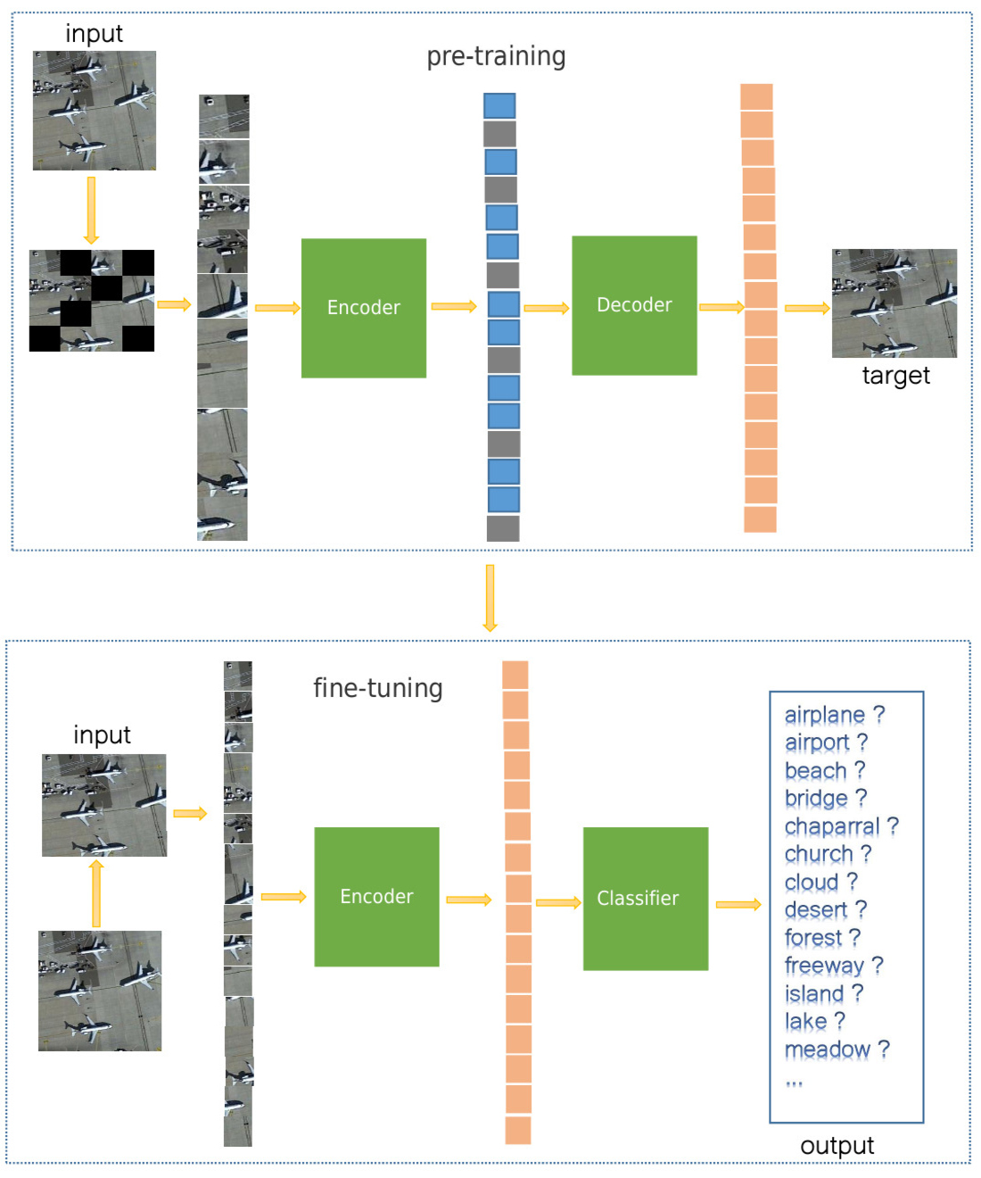
The self-supervised learning network proposed in this paper is essentially an autoencoder structure, as shown in Figure 1. Rumelhart et al. [46] proposed the concept of Auto Encoder (AE) in 1986 and applied it to high-dimensional complex data processing, which promoted the development of neural networks. He et al. [47] proposed a masked autoencoder for self-supervised learning. AE is an unsupervised learning algorithm, and the network structure generally consists of two parts: an encoder for feature extraction and a decoder for target reconstruction. Generally speaking, the structure of the encoding and decoding of the autoencoder is symmetric, but the autoencoder framework designed in this paper is an asymmetric structure. The encoder can label the order of image patches by position embedding. In addition, it can also process the mask and mask token of the image patches, and the decoder does not contain these functions.

A. VIT

The Vision Transformer (VIT) model is developed based on the transformer model and is widely applied in computer vision. The Transformer was introduced by Vaswani et al. [48] to overcome the defects that recurrent neural networks cannot be parallelized in natural language processing (NLP), which consists of an encoder and a decoder. In the encoding stage, the words in the sentence are firstly converted into word vectors, then the global self-attention feature map is obtained through the self-attention module, residual connection, and layer normalization. Finally, the output of the encoder is obtained by the feedforward network, residual connection, and layer normalization. The VIT model proposed by Dosovitskiy et al. [49] is the first time that the encoder structure of the Transformer is directly used for image classification, laying a solid foundation for the development of the transformer in computer vision. To adapt to the structure of the input data of the transformer, the images need to be divided into non-overlapping image patches in the VIT model, and then the image patches are flattened and embedded in position encoding. Finally, a one-dimensional vector is obtained. The application of the transformer in computer vision usually uses this method to input images or feature maps. For the image classification task, a classifier is usually connected in the end to map the output features by the encoder to the scene category. In the process of scene classification, the useful information is usually concentrated in a specific area. The traditional CNN architecture is a filter based on a local receptive field, which treats each pixel equally. However, for the scene classification of the whole image, the contribution of each pixel in the image is different. For example, airports are mainly identified according to the aircraft contained in the image, while commercial and residential areas are identified according to the geometric outline, texture features, and spatial arrangement of buildings. VIT model adopts a multi-head self-attention (MSA) mechanism, which can automatically learn the contribution of each pixel to scene classification, which is more in line with the image recognition process of the real human visual system.

B. Encoder

As shown in Figure 1, the left side of the encoder is composed of the standard VIT structure, in which the classification header has been removed, and the function of the right part is to restore the number of image patches. During the data processing of the encoder, we discard the masked image patches. Here, we add the positional embeddings to the output features of VIT and mask tokens of the image, respectively, and concatenate them together, then the length of concatenated feature vectors is equal to the total number of image patches. Finally, the output features are sent to the decoder. The main structure of VIT is composed of an embedding layer and a transformer encoder. The transformer encoder cannot process two-dimensional images directly, and can only accept one-dimensional vectors as input. Therefore, when using VIT, it is necessary to map the two-dimensional matrix to the one-dimensional vector.

We suppose that the size of the input remote sensing image P is $c\times h\times w$, where c represents the number of channels, h represents the height, and w represents the width. We uniformly divide the image into non-overlapping image patches, and the size is $c\times h_p\times w_p$, $h_p$ and $w_p$, usually set to 16, then the total number of image patches $m=hw/h_p{w}_p$. All the image patches are concatenated together to form a patch sequence ($P_1$, $P_2$, …, $P_m$) with a length of m, and then the patch sequence is input into the linear embedding layer and projected into a vector of dimension N, then the vector can be used as input data of the transformer encoder. The process of linear embedding can be expressed by the following formula:

$$\begin{array}{c}{L}_0=[P_{1}E;P_{2}E;\dots ;P_{m}E]+E_{pos},E\in R^{\left(h_p{w}_{p}c\right)\times d},\\ E_{pos}\in R^{(m+1)\times d}\end{array}$$

(1)

where E represents a learnable embedding matrix and $E_{pos}$ represents position encoding. Since the transformer’s self-attention is disordered, the patch sequence ($P_1$, $P_2$, …, $P_m$) is regarded as a group of disordered patches. To maintain the relative spatial position of the patch in the raw image, $E_{pos}$ is used to embed the position information into the patch sequence. $[P_{1}E;P_{2}E;\dots ;P_{m}E]$ represents that we concatenate the $P_{1}E$, $P_{2}E$, …, and $P_{m}E$ together. The position encoding method adopted in this paper can be expressed by the following formula [50]:

$$\begin{array}{c}{E}_{pos\left(2i\right)}=sin(pos/{\mathrm{10,000}}_{2i/d})\\ E_{pos(2i+1)}=cos(pos/{\mathrm{10,000}}_{2i/d})\end{array}$$

(2)

where $pos$ represents the regional position index of the image and d represents the position encoding dimension, i represents the ith dimension of the position encoding vector.

The paper adopts a random mask-based self-supervised learning framework to predict deleted patches from visible unmasked patches. The transformer encoder only processes the visible patches, so the masked patches are removed from the vector $L_0$ after the linear embedding operation. If the number of patches to be masked is n, then the number of visible patches is $m-n$. After this step, the patch sequence $L_1$ can be expressed by the following formula:

$$\begin{array}{c}{L}_1=[P_1;P_2;\dots ;P_{m-n}]\end{array}$$

(3)

$[P_1;P_2;\dots ,P_{m-n}]$ represents that we concatenate the $P_1$, $P_2$, …, and $P_{m-n}$ together. The transformer encoder takes $L_1$ as the input sequence for feature extraction. The Transformer encoder consists of several layers with same structure. Each layer mainly includes a MSA module and a multi-layer perceptron (MLP) module with. To ensure the consistency of data distribution, the data must be processed by a normalization layer before being input into each module. In addition, a residual skip connection is used in each module. The perceptron layer consists of two fully connected layers, then nonlinear mapping is performed between the two dense layers through a GeLU activation function. The transformer encoder is made up of several such units. If the number of such units is k, the calculation process of the transformer encoder can be expressed as following:

$$\begin{array}{c}{L}_k^{\prime }=MSA\left(LN(L_k-1)\right)+L_k-1,k=1,2,\dots ,K\\ L_k=MSA\left(LN\left(L_k^{\prime }\right)\right)+L_k^{\prime },k=1,2,\dots ,K\end{array}$$

(4)

where $L_k$ represents the kth layer of the transformer encoder, $LN$ represents the abbreviation of Layer Norm, and $MSA$ represents the abbreviation of MSA.

The last layer of the encoder is to integrate the output of the features by the transformer encoder and the features of the masked patches while embedding their position information separately. Finally, they are concatenated and sent to the decoder for the reconstruction of the discarded image patches. The masked patches feature can be represented by a trainable and shared mask token. The whole process can be expressed as follows:

$$\begin{array}{c}T=[p_1^{\prime };p_2^{\prime };\dots ;p_n^{\prime }]+E_{pos}^M\\ L_{cat}=[L_k+E_{pos}^V;T]\end{array}$$

(5)

In the above formula, $p_n^{\prime }$ represents the nth mask token, $E_{pos}^M$ represents the position embedded feature of the image patches that are masked, $L_k$ represents the feature vector output by the Transformer encoder, and $E_{pos}^V$ represents the position embedded feature of the image patches that are not masked. $L_{cat}$ represents that the mask token of the embedded position information and the previously extracted features are concatenated together, and the length of the features vector is exactly equal to the number of all image patches.

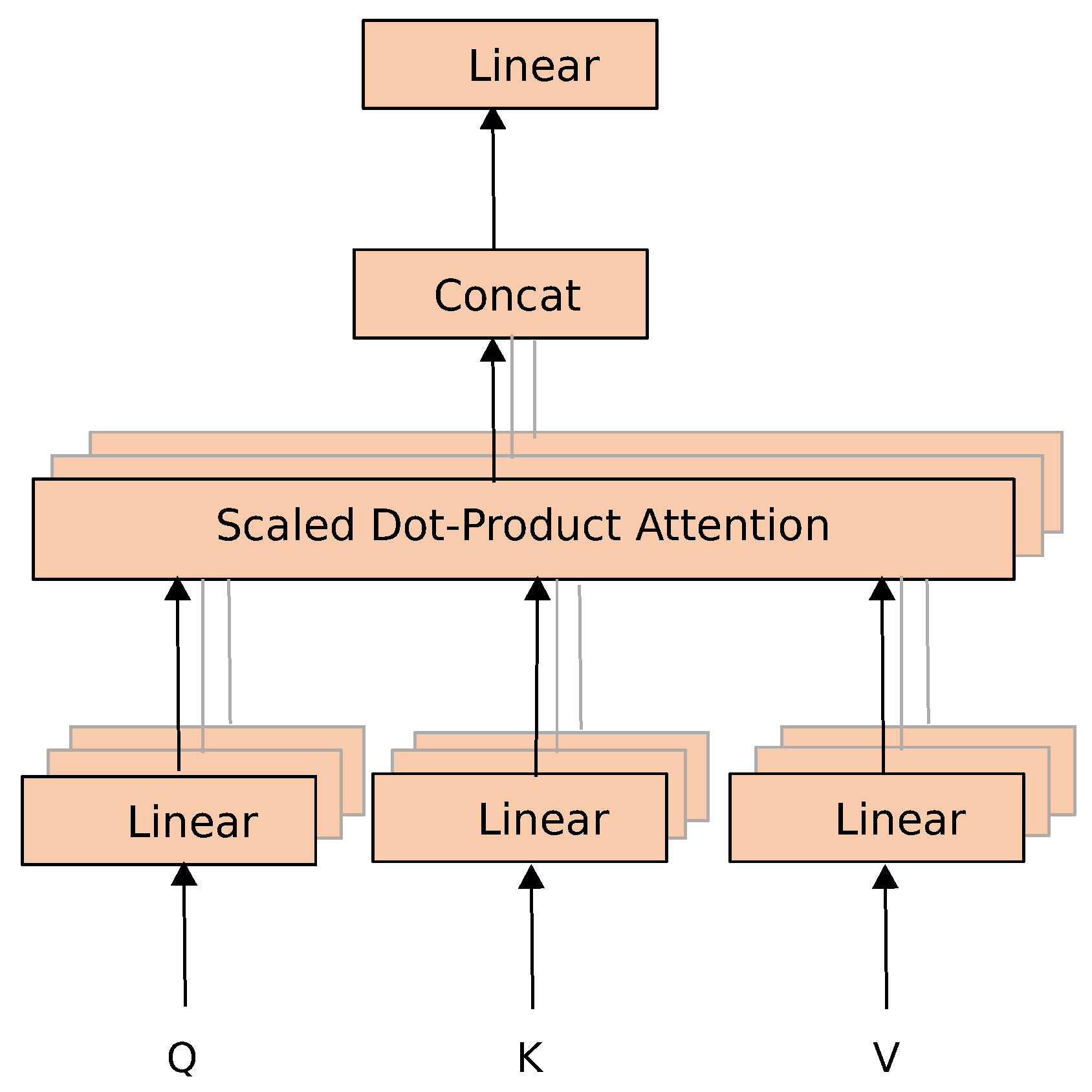
C. MSA mechanism

MSA is a key part of VIT, and the structure is shown in Figure 2. Firstly, three learnable matrices that represent different weights are used to transform the input matrix of the encoder to obtain the query matrix Q, the key matrix K, and the value matrix V. Then, through the scaled dot-product attention, the self-attention feature map is calculated. The ultimate goal of multi-head self-attention is to obtain multi-independent attention feature maps, which are realized by multi-group transformation matrices. Finally, the multi-head attention feature map is obtained by concatenating different attention feature maps. The formula for calculating attention features is as follows

$$\begin{array}{c}Attention(Q,K,V)=softmax\left(\frac{Q{K}^T}{\sqrt{d_k}}\right)V\end{array}$$

(6)

Among them, Q, K, and V are two-dimensional matrices composed of vectors, the dot product between the matrix Q and the transpose of the matrix K represents a correlation matrix. Because Q and K come from the transformation of the same matrix, the correlation matrix can describe the correlation between the input vectors. To avoid the vanishing gradients caused by the softmax operation, a coefficient is used to scale the correlation matrix. $\sqrt{d_k}$ represents a coefficient, where $d_k$ represents the dimension of the vector k, which is used to scale the output. The activated correlation matrix is dot-multiplied with V to obtain the global self-attention map.

D. Decoder

The main structure of the decoder is the same as that of the transformer encoder in the encoder, which consists of a stack of MSA modules and MLP modules. The role of the decoder is to recover the masked image patches by predicting a vector of pixel values for each masked token. The fully connected layer in the end is used to map the number of feature channels output by the transformer encoder to be consistent with the number of pixels in the masked image patches. Finally, the predicted mask patch pixel value is filled to its original position, thus completing the reconstruction of the entire image. It is worth emphasizing that in the training process, our loss function only calculates the mean square error of the predicted pixels value and the original image pixels value for the masked image patches because we only predict the pixels value of the mask token.

E. Remote Sensing Image Scene Classification

When the training of the self-supervised learning model has been completed, we use the VIT module in the encoder to extract the features and add a classifier in the end of the network, they form a scene classifier together. The dimension of the output feature is equal to the scene categories. Although the structure of the scene classifier is similar to the VIT module in the encoder, there lies a significant difference between them. In the pre-training stage, the VIT module only needs to process the image patches that are not masked, but all the image patches need to be processed in the classifier, and the masked image patches are no longer removed.

4. Experiments and Analysis

A. Datasets description

In this experiment, we used 11 kinds of different datasets, each of which is described in detail in

Table 1. The experiment datasets.

Datasets	Image Number Perclass	Number of Scene Categories	Total Number	Size	Data Sources
UC Merced [13]	100	21	2100	256 × 256	Aerial orthoimagery
WHU-RS19 [50]	50∼61	19	1005	600 × 600	Google Earth
SIRI-WHU [51]	200	12	2400	200 × 200	Google Earth
RSI-CB256 [52]	about 690	35	24,000	256 × 256	Google Earth and Bing Maps
RSSCN7 [53]	400	7	2800	400 × 400	Google Earth
RSC11 [54]	about 100	11	1232	512 × 512	Google Earth
OPTIMAL-31 [55]	60	31	1860	256 × 256	Google Earth
PatternNet [56]	800	38	30,400	256 × 256	Google Earth
GID [57]	-	-	-	6800 × 7200	Gaofen-2
NWPU-RESISC45 [4]	700	45	31,500	256 × 256	Google Earth
AID [58]	220∼420	30	10,000	600 × 600	Google Earth

. Among them, UC Merced, WHU-RS19, SIRI-WHU, RSI-CB256, RSSCN7, RSC11, OPTIMAL-31, PatternNet, and GID datasets are used for pre-training of self-supervised learning models. The first 8 data sets are public remote sensing scene classification data sets with labels, with a total of 65,797 images. In the pre-training process, labels are not required. The image size is uniformly resized to 224 × 224. We name it the public image dataset (PID). Although unlabeled scene classification datasets have also been used in previous studies to train self-supervised models, these datasets are manually produced and carefully selected to identify specific kinds of scenes. The categories of scenes included are very limited, the number of samples is not large, and the production cost is very expensive. In a word, the unlabeled datasets are not naturally generated. GID dataset (Gaofen image dataset) is a remote sensing image’s semantic segmentation dataset produced by Wuhan University, which contains 150 high-resolution Gaofen-2 images (the image size 6800 × 7200) obtained from more than 60 cities in China. These images cover a geographical area of more than 50,000 square kilometers. Images in GID have high intra-class similarity and low inter-class separability. We select images from which the distribution of ground objects is relatively uniform as training samples. Because the uneven samples will lead to a large number of redundant datasets. For example, most areas of the whole image are covered by water, farmland, and forests with single texture features, which means that the distribution of ground objects is uneven. Too many samples like these images will not help improve classification performance, but will lead to an increase in calculation cost. For training samples, each image is cut into non-overlapping image patches with the size of 224 × 224. In order to keep consistent with the number of images selected from public remote sensing scene classification data sets, we randomly selected 65,797 images from the generated image patches for the pre-training process of the self-supervised learning model. We combine PID and GID to construct a large-scale unlabeled dataset with a total of 131,594 images, which we name as Large Scale Image Dataset (LSID). In addition, to verify the performance of the self-supervised learning method, we selected two complex scene classification datasets as train datasets and test datasets for scene classification tasks, namely the NWPU-RESISC45(NWPU) and AID datasets, the detailed descriptions are shown in Table 1.

B. Experiment Setup

Our experiments are composed of two groups. The purpose of the first group is to verify the performance of our proposed self-supervised learning network. We conduct pre-training experiments on the LSID dataset, and then perform the scene classification experiment on the NWPU dataset and AID dataset, respectively, which we call self-supervised learning scene classification (SSLSC). Meanwhile, we also exploit the VIT model pre-trained on the natural dataset to conduct scene classification experiments on the NWPU dataset and AID dataset to compare and analyze the advantages of the SSLSC method. We also use the VIT model for scene classification based on the SSLSC method, which has the same structure as the VIT model used for pre-training on natural datasets. The other group of the experiment is designed to compare the performance of our proposed self-supervised learning network on the PID and AID datasets, the models are pre-trained on these two datasets, respectively. Then, we fine-tune the model on the NWPU dataset and AID dataset for scene classification. In the pre-training stage of the SSLSC method, we set the learning rate to 1.5 × 10${}^{-4}$, the epoch to 500, and the batch to 64. The depth of the transformer encoder in the encoder is set to 12, and it is set to 4 in the decoder. The random mask ratio of the image patches is set to 0.75, which means 75% of the image patches are randomly discarded for each image during the encoding stage and then reconstructed during the decoding stage. In the model fine-tuning stage of the SSLSC method, the learning rate is set to 1 × 10${}^{-3}$, the epoch is set to 200, the batch is set to 64, and the depth of the transformer encoder in the encoder is set to 12. The attention head is set to 12 and the embedding layer dimension is set to 768 in all encoders. For the NWPU data set, the training ratio is set to 10% and 20%, whereas for the AID data set, the training ratio is set to 20% and 50%, respectively. To obtain reliable results, the experiments were repeated 10 times during scene classification. We choose the overall accuracy and confusion matrix to evaluate the performance of the model and finally calculate the average of the overall accuracy of 10 experiments as the accuracy of the model. In addition, we use the best model in the training process to calculate the confusion matrix. The settings of these parameters of the VIT model pre-trained on the natural dataset are consistent with the VIT model fine-tuned by SSLSC, and we choose the ViT-B_16 model trained on the ImageNet2021 and ImageNet-21 data sets as the pre-trained model. All our experiments are conducted on a computer, which has 2.70 GHz × 12 core CPU with 32GB memory, configured with a GeForce GTX 1080 Ti graphics card with 11GB memory capacity.

C. Experimental results of SSLSC

To validate the effectiveness of our proposed method, we compare it with some other state-of-the-art methods in this section. As is known to all, the performance of the method based on deep learning in scene classification far surpasses the traditional machine learning method based on handcrafted feature extraction. Therefore, the methods used for comparison are all based on deep learning.

(1) Result on LSID dataset: LSID is a large-scale unlabeled training dataset that we constructed to train the self-supervised learning task. The goal of this stage is to learn the features of the image from the unmasked image patches, so as to recover the pixels of the masked image patches. The final pre-trained model can be used as a feature extractor for fine-tuning in downstream scene classification tasks. We can show the reconstruction effect of the model on the pixels of the masked image patches. The better the reconstruction effect of image pixels, the more representative the features extracted by the encoder of the self-supervised learning framework, and it also shows that the pre-trained model is suitable as a feature extractor for downstream tasks. Now, we randomly select an image from each of five typical scene categories which represent mountain, dense residential, commercial area, church, and airport to restore the image pixels and evaluate the feature extraction ability of the proposed model. We carried out the experiments on the NWPU dataset and AID dataset, respectively.

The experimental results on the two datasets are shown in Figure 3 and Figure 4, respectively. The images of five scene categories are represented from left to right, which are mountain, dense residential, commercial area, church, and airport. The images from top to bottom represent the original image, the masked image, and the reconstructed image in turn. Comparing the results in Figure 3 and Figure 4, we can find that the discarded pixels can be well recovered. In particular, through the comparison between the original image and the reconstructed image, we can see that the latter can be consistent with the former in color and texture. Through analysis, we can draw a conclusion that the encoder of the self-supervised learning framework proposed in this paper can extract representative image features, which have good robustness. The pre-trained model can well predict the discarded pixels of the masked image patches on the NWPU dataset and AID dataset.

(2) Result on NWPU dataset:

Table 2. OA (%) of eighteen kinds of methods and our method under the training ratio of 10% and 20% on NWPU dataset.

Method	Training Ratio
	10%	20%
AlexNet [20]	76.69 ±  0.21	79.85 ±  0.13
GoogleNet [22]	76.19 ±  0.38	78.48 ±  0.26
VGGNet-16 [21]	76.47 ±  0.18	79.79 ±  0.15
D-CNN based on AlexNet [60]	85.56 ±  0.20	87.24 ±  0.12
D-CNN based on GoogleNet [60]	86.89 ±  0.10	90.49 ±  0.15
D-CNN based on VGGNet-16 [60]	89.22 ±  0.5	91.89 ±  0.22
Siamese ResNet50 [61]	-	92.28
EfficientNet [59]	90.91 ±  0.16	94.37 ±  0.14
ADSSM [67]	91.69 ±  0.22	94.29 ±  0.14
SF-CNN [68]	89.89 ±  0.16	92.55 ±  0.14
DNE [69]	-	96.01
Hydra [66]	92.44 ±  0.34	94.51 ±  0.21
ResNeXt-101+MTL [44]	91.91 ±  0.18	94.21 ±  0.15
RCOVBOVW [62]	90.25 ±  0.13	92.37 ±  0.18
EMTCAL [63]	91.63 ±  0.19	93.65 ±  0.12
T-CNN [64]	90.25 ±  0.14	93.05 ±  0.12
ResNet-101+EAM [65]	91.91 ±  0.12	94.29 ±  0.09
ViT-B_16 [224 × 224]	91.89 ±  0.43	93.26 ±  0.1
SSLSC+LSID	92.68 ±  0.15	94.73 ±  0.11

shows the overall accuracy comparison of scene classification, and Figure 5 shows the classification confusion matrix, all of which are based on the NWPU dataset. The methods in Table 2 mainly include the current mainstream CNN-based methods and their variants. For example, AlexNet [20], GoogleNet [22], VGGNet-16 [21] and EfficientNet [59] are all classic CNN networks. D-CNN with AlexNet [60], D-CNN with GoogleNet [60], D-CNN with VGGNet-16 [60], Siamese ResNet50 [61] and ResNeXt-101+MTL [44] are variants of AlexNet, GoogleNet, VGGNet-16, ResNet50 and ResNeXt-101, respectively. In addition, we also list some excellent methods proposed in the past two years and compare their classification accuracies. These methods include RCOVBOVW [62], EMTCAL [63], T-CNN [64], and ResNet-101+EAM [65]. From Table 2, it can be observed that the overall accuracy of our method surpasses all methods. Among the previous methods listed in the table, Hydra [66] has the best performance on the 10% training dataset, with an overall accuracy of 92.44%, but our method has an overall accuracy of 92.68%, which is 0.24% higher than the former. Hydra [66] is also the method that performs best on 20% of the training dataset, the overall accuracy reaches 94.51%, but our method has an overall accuracy of 94.73%, which is 0.22% higher than the former. It is worth emphasizing that ResNeXt-101+MTL [44] is also a self-supervised learning method, and on 10% and 20% training datasets, the overall accuracy is 91.91% and 94.21%, respectively. Compared with this, our overall accuracy is improved by 0.77% and 0.52%, respectively. In addition, ViT-B_16 [224 × 224] represents the Vision Transformer framework, the input image size is 224 × 224, and the image is divided into 16 × 16 image patches. We use the pre-trained model, which is trained on two natural datasets (ImageNet2021 and ImageNet-21), to fine-tune for the scene classification task, the overall accuracy is 91.89% on 10% of the training dataset, and which is 93.26% on 20% of that dataset. It is obviously that our overall accuracy is improved by 0.79% and 1.47%, respectively.

In addition, Figure 5 shows the confusion matrix for scene classification on the NWPU dataset. From Figure 5, we can observe that the proposed model can identify most of the scene categories correctly, their overall accuracy exceeds 90%, especially for the images with scene categories of airplane, chaparral, circular farmland, cloud, harbor, parking lot, snowberg, and storage tank, the overall accuracy reaches 100%. However, the recognition accuracy is relatively low for some scene categories. For example, for church, commercial area, mountain, palace, railway station, and wetland, their overall accuracies are 87%, 89%, 87%, 84%, 89% and 89%, respectively. Through further analysis, we can summarize the reasons for the lower recognition accuracy of these scene categories. Figure 5 shows that 8% of the churches were mistakenly classified as palaces, while 11% of the palaces were mistakenly classified as churches, because churches and palaces have many similarities in architectural structure. Overall, 6% of the mountains were identified as deserts because the sparsely vegetated mountains had a similar color to the desert, and 7% of the railway stations are identified as railways. According to common sense, there are generally dense railways around the railway station, and they are easy to identify as railways. Additionally, 6% of wetlands were identified as lakes because both wetlands and lakes contain water bodies, and wetlands are easily classified as lakes when there is a lot of water in them.

(3) Result on AID dataset:

Table 3. OA (%) of twenty kinds of methods and our method under the training ratio of 20% and 50% on AID dataset.

Method	Training Ratio
	20%	50%
CaffeNet [58]	86.86 ± 0.47	89.53 ± 0.31
VGG-VD-16 [58]	86.59 ± 0.29	89.64 ± 0.36
GoogLeNet [58]	83.44 ± 0.40	86.39 ± 0.55
DenseNet121 [71]	93.76 ± 0.23	94.73 ± 0.26
DenseNet169 [71]	92.43 ± 0.36	94.17 ± 0.33
VGG19 [72]	87.73 ± 0.25	91.71 ± 0.42
ResNet50 [72]	92.39 ± 0.15	94.69 ± 0.19
InceptionV3 [72]	93.27 ± 0.17	95.07 ± 0.22
HW-CNNs [73]	-	96.98 ± 0.33
SF-CNN [68]	93.60 ± 0.12	96.66 ± 0.11
CNNs-WD [70]	-	97.24 ± 0.32
RSFJR [74]	-	96.81 ± 1.36
GBN [75]	92.20 ± 0.23	95.48 ± 0.12
CNN-CapsNet [76]	93.79 ± 0.13	96.32 ± 0.12
CMC [26]	-	95.58
ResNeXt-101+MTL [44]	93.96 ±  0.11	96.89 ±  0.18
EMTCAL [63]	94.69 ±  0.14	96.41 ± 0.23
T-CNN [64]	94.55 ±  0.27	96.72 ± 0.23
ResNet-101+EAM [65]	94.26 ±  0.11	97.06 ± 0.19
ViT-B_16 [224 × 224]	93.54 ± 0.25	96.25 ± 0.17
SSLSC+LSID	94.13 ± 0.29	97.44 ± 0.14

and Figure 6 are the scene classification results on the AID dataset. Similar to Table 2, the methods compared in Table 3 mainly include the current mainstream CNN-based methods and their variants. We can see that our method has the highest overall accuracy than other methods when the training ratio is set to 50%. The accuracies are 94.13% and 97.44% on the 20% and 50% training datasets, respectively. In the previous methods, on 20% training dataset, the method with the highest accuracy is EMTCAL [63], and the overall accuracy reaches 94.69%. Unfortunately, the accuracy of our method is 0.56% lower than that. On the 50% training dataset, the method with the highest accuracy is CNNs-WD [70], and the accuracy reaches 97.24%. Although CNNs-WD [70] is already excellent, the accuracy is 0.46% lower than that of our method. In addition, we also compare with other self-supervised learning methods and Vision Transformer, among which, CMC [26] and ResNeXt-101+MTL [44] are self-supervised learning methods. On the 50% training dataset, the overall accuracy of CMC [26] is 95.58%, and the overall accuracy of ResNeXt-101+MTL [44] is 96.89%, but our method outperforms them by 1.86% and 0.55%, respectively. On two different rates of a training dataset, the overall accuracy of Vision Transformer is 93.54% and 96.25%, which are 0.59% and 1.19% lower than our method. 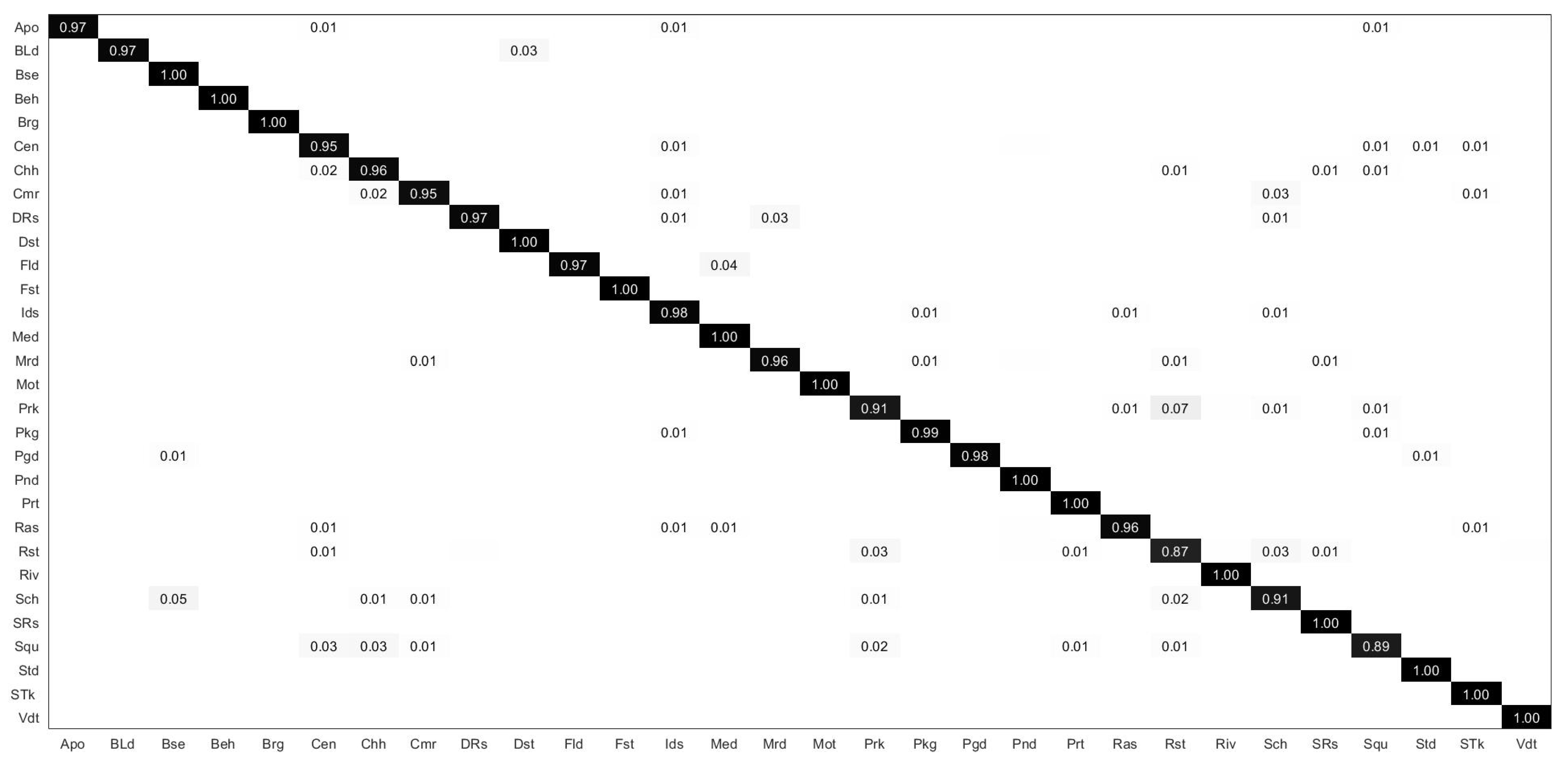Figure 6 shows the confusion matrix. It can be observed from Figure 6 that nearly half of the scene categories have an overall accuracy of 100%. They are baseball field, beach, bridge, desert, forest, meadow, mountain, pond, port, river, sparse residential, stadium, storage tanks, and viaducts. Only two scene categories have overall accuracies below 90%, resort and square, with accuracies of 87% and 89%, respectively. Through further analysis, it can be seen that 3% of the resorts are identified as parks, and 3% of the resorts are identified as schools. In addition, 3% of squares are identified as center, and 3% of squares are identified as church. Resort, park, and square are all interspersed with trees and grass among the sparse buildings, there are some similarities in spectral and spatial arrangement. Square, center, and church have a common feature that they all contain circular building structures, then the geometric shapes shown in the images have certain similarities, so these scene categories are very easy to be misclassified. Compared with the current state-of-the-art methods, this shows that our method is superior to most of the previous methods.

D. Comparison of Classification Accuracies Based on Different Pre-Training Datasets

As described in the dataset description section above, the GID dataset is an unlabeled data set constructed by directly cropping the visible light band of the Gaofen-2 remote sensing image into image patches. The generation process requires no manual intervention and can be completed in just a few minutes. The PID dataset is produced by integrating many public scene classification datasets. Although we have not used labels, the construction process of these datasets is very complex, and they are produced by careful manual selection. Labeling datasets requires strong professional knowledge and rich experience, and it also takes a long time. Therefore, so far, there are not enough labeled datasets that can be used for scene classification in remote sensing. In this section, we use GID and PID datasets to train the self-supervised learning model, respectively, then fine-tune the pre-trained model on the labeled scene classification dataset, and evaluate the performance of the model with overall accuracy. Our experiments are performed on the NWPU and AID datasets, respectively. Additionally, we also compare the results with ViT-B_16 [224 × 224] and SSLSC+LSID.

Table 4. OA (%) of experiment on NWPU with different pre-training datasets.

Method	Training Ratio
	10%	20%
SSLSC+GID	87.21	91.33
SSLSC+PID	87.45	91.73
ViT-B_16 [224 × 224]	91.89	93.26
SSLSC+LSID	92.68	94.73

and

Table 5. OA (%) of experiment on AID with different pre-training datasets.

Method	Training Ratio
	20%	50%
SSLSC+GID	91.28	95.10
SSLSC+PID	91.74	94.90
ViT-B_16 [224 × 224]	93.54	96.25
SSLSC+LSID	94.13	97.44

show the experimental results. It can be seen from Table 4 that the overall accuracy of SSLSC+PID is higher than that of SSLSC+GID, which is 0.24% higher on 10% training set and 0.4% higher on 20% training set respectively. Compared with SSLSC+LSID, the overall accuracy of SSLSC+PID is 5.23% and 3% lower on the 10% and 20% training sets, respectively. Table 5 shows the results on the AID dataset. The overall accuracy of SSLSC+PID is 0.46% higher than that of SSLSC+GID on 20% of the training rate. However, on 50% training rate, the results are exactly the opposite. The overall accuracy of SSLSC+PID is 0.2% higher than that of SSLSC+GID. Compared with SSLSC+LSID, the overall accuracy of SSLSC+PID is 2.39% and 2.54% lower on the 20% and 50% training sets, respectively. In addition, both the metrics of SSLSC+GID and SSLSC+PID in Table 4 and Table 5 were lower than ViT-B_16 [224 × 224]. The ViT-B_16 [224 × 224] is a traditional supervised learning framework. In this experiment, we choose the model trained on ImageNet2021 and ImageNet-21 datasets, which have more than one million labeled samples and contain 1000 scene categories as the pretrained model. However, in the comparison experiments, both PID and GID datasets contain 65,797 samples, and compared with natural image datasets, these two datasets are much smaller in scale. Hence, the overall accuracy of ViT-B_16 [224 × 224] is lower. The LSID dataset is composed of the PID dataset and the GID dataset. In all combinations in Table 4 and Table 5, the performance of SSLSC+LSID outperforms the other methods.

Through further analysis, it can be found that the PID dataset has several advantages over the GID dataset. First of all, the PID dataset has high inter-class dissimilarity and low inter-class similarity. Because it is manually selected, the distribution of ground objects in each image is more in line with the corresponding scene category. Secondly, for the downstream scene classification task, the distribution of scene categories in the PID dataset is more uniform, which can ensure that each scene category has a certain amount of data. Taking churches as an example, the GID data comes from cities in China, where the number of churches is relatively small. Finally, the PID dataset comes from a wide range of sources, some from aerial orthophotos, some from Google Earth, etc., which included different types of sensors and different sizes of spatial resolution. Therefore, the overall accuracy on the PID dataset is slightly higher in most cases. In general, the accuracy difference between SSLSC+GID and SSLSC+PID is not great, but the GID dataset is very easy to obtain, which has great advantages in applying large-scale unlabeled datasets to the training of self-supervised learning.

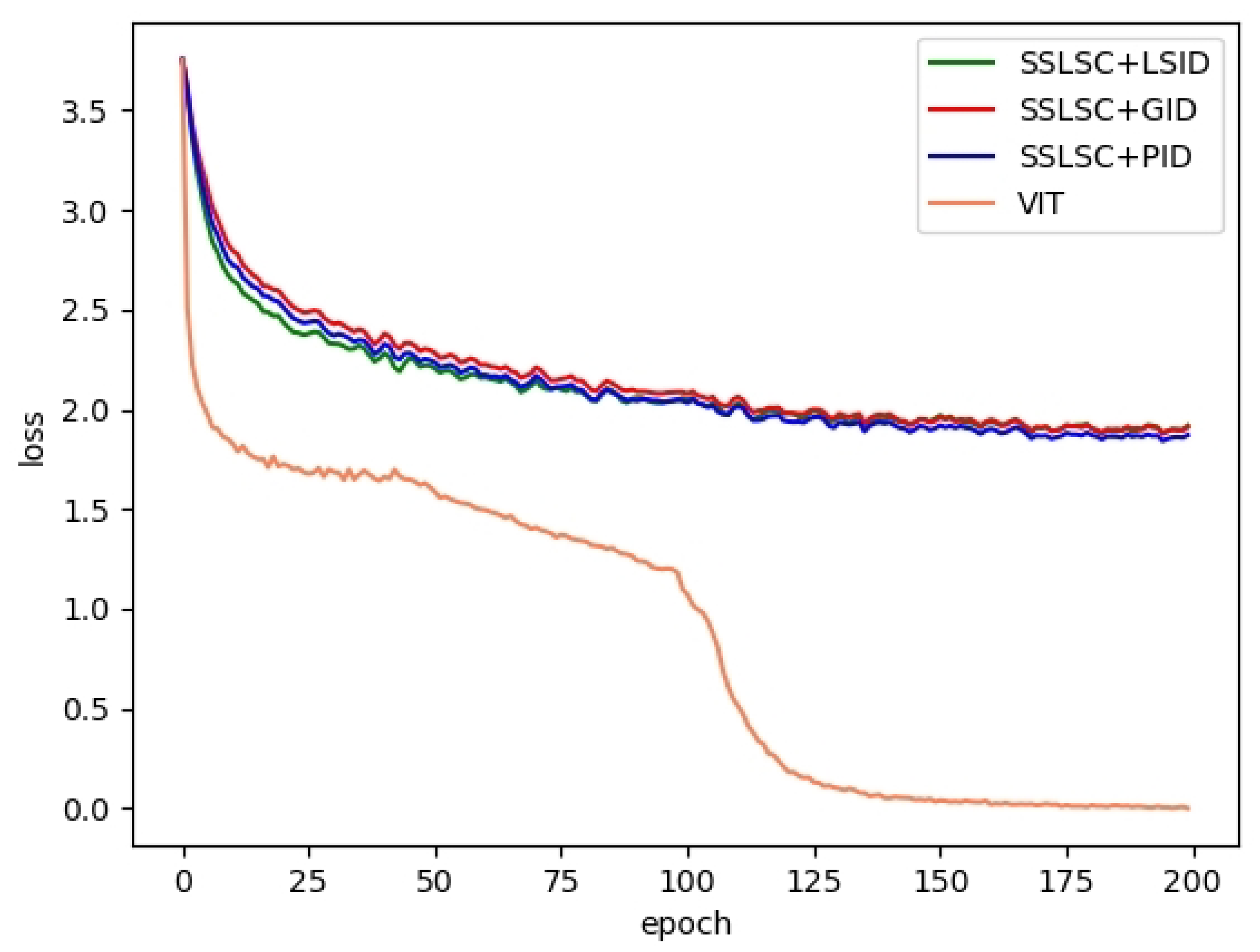
E. Effects of different pre-training models on training loss

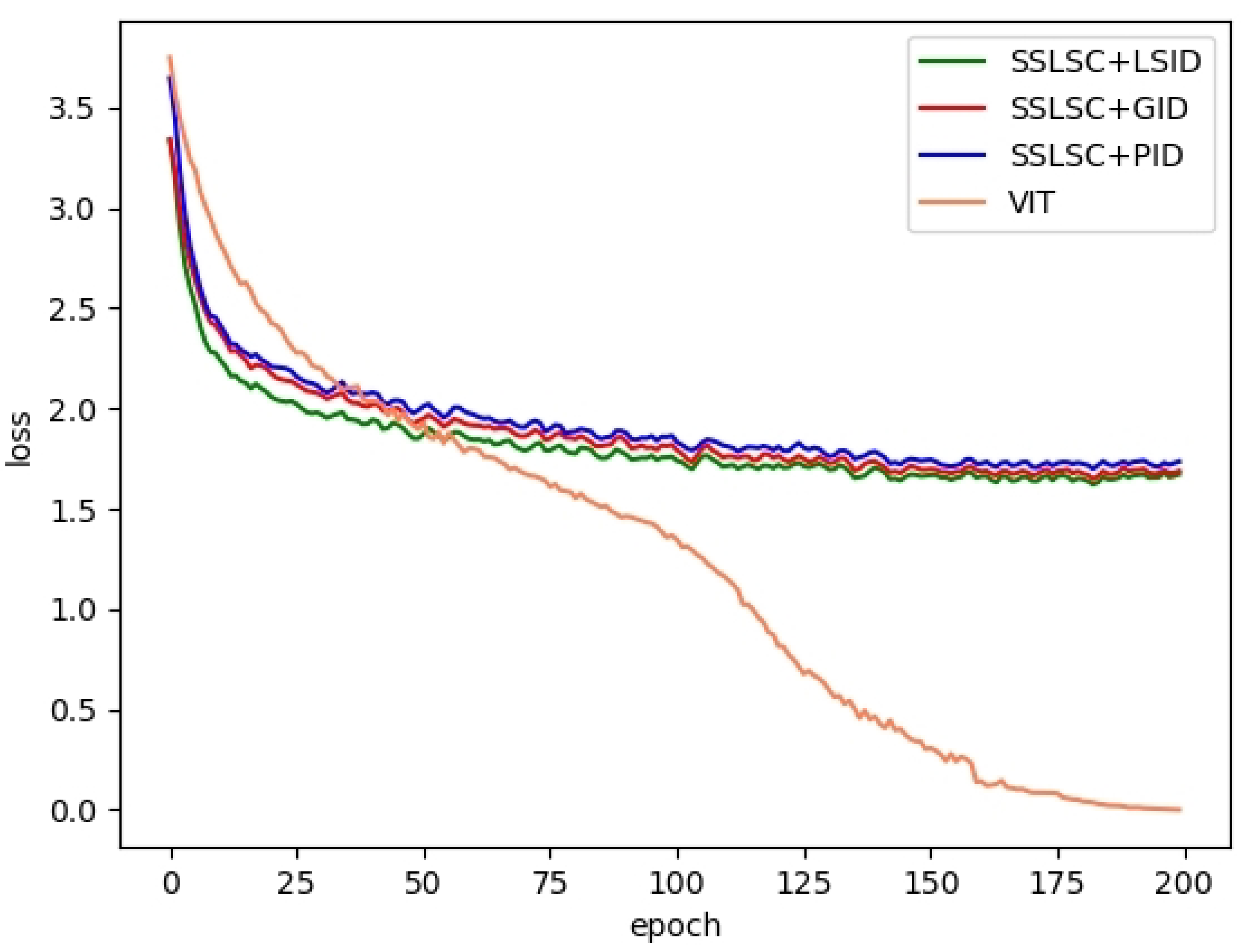
In this section, we mainly analyze the effects of different pre-training models on training loss. LSID, GID, and PID represent three different pre-training datasets, respectively. We pre-train the self-supervised model on these three datasets to form three different kinds of pre-trained models. Then, we fine-tune the models on the downstream task of remote sensing scene classification; SSLSC + LSID, SSLSC + GID, and SSLSC + PID represent these three different methods, respectively. VIT stands for Vision Transformer, which uses a model (i.e., ViT-B_16 [224 × 224]) pre-trained on a natural dataset. We analyze the effects of different pre-training models on training loss in the process of training the scene classification model. Our experiments are performed on the NWPU dataset and the AID dataset, the rate of the training set is set to 20% and 50%, respectively, and the epoch is set to 200. The results are shown in Figure 7 and Figure 8. We can observe from Figure 7 and Figure 8 that the changing trend of the loss value of SSLSC+LSID, SSLSC+GID, and SSLSC+PID on the two data sets is almost the same, and the loss value decreases rapidly with the progress of training. When the epoch is greater than 75, the loss value only fluctuates in a small range, and the model has converged. However, compared with our method, the changing trend of the loss value of VIT is quite different. On the NWPU dataset, the loss value tends to stabilize when the epoch value is about 150. On the AID dataset, the model starts to converge when the epoch value is greater than 170. In addition, the variation range of losses is also quite different on two different pre-trained models. On the pre-training model based on unlabeled remote sensing data sets, the loss range is smaller, between 1.5 and 4. On pre-trained models based on natural data sets, the loss variation is much larger, between 0 and 4. Which may be one of the reasons why our method can reach convergence first. In general, compared with the VIT model, which is pre-trained on the natural dataset, our method can reach convergence first, which can save training time. Further analysis shows that an unlabeled remote sensing dataset we used in the pre-trained stage is consistent with the scene classification dataset in the downstream task in terms of spectrum, texture, and geometric structure. Therefore, our method can learn more representative image representations, convergence can be achieved with fewer iterations. In addition, the dataset we used does not need manual annotation, so we can complete the task of scene classification on remote sensing image datasets more efficiently.

5. Conclusions

In this study, we proposed a scene classification method for a remote sensing image based on a self-supervised learning framework, which can use an unlabeled dataset to learn the representation of the image, and then transfer the learned knowledge to the scene classification task. The self-supervised learning framework consists of an encoder and a decoder. The function of the encoder is to process the unmasked image patches, learn the feature representation of the image, and then combine them with the mask token of the image to form a joint encoding. The role of the decoder is to reconstruct the pixels of the masked image patches. The whole process is trained on unlabeled images, and the training dataset is constructed based on Gaofen-2 remote sensing images and public scene classification datasets. Then, we transfer the parameter weights learned by the encoder to fine-tune the scene classification task. The scene classification experiments were carried out on two public and challenging datasets (NWPU dataset and AID dataset), respectively. We used the OA of the classification and the confusion matrix to evaluate the performance of the model and compared it with the current mainstream scene classification methods. We can draw a conclusion that our method is superior to most state-of-the-art methods. We conducted comparative experiments on two different unlabeled datasets, one of which was integrated based on the public hand-crafted scene classification datasets, and the other was randomly generated based on Gaofen-2 satellite imagery. Through analysis, our method can also achieve good performance on an unlabeled dataset that was generated without human intervention. Finally, we analyzed the effects of different pre-training models on training loss. The results show that our method can reach convergence with fewer iterations, then we can save the training time. In conclusion, our method can overcome the dependence on large-scale labeled datasets of the traditional supervised learning methods. The above experiments prove that our method has obvious advantages over other methods

In future research, we will consider using multi-source data to randomly generate unlabeled datasets to train the self-supervised learning model and then apply it to the scene classification of remote sensing images. These datasets include different spatial resolutions, different band combinations, different sensors, and different countries and regions, so as to further improve the accuracy of scene classification.