A Dynamic Effective Class Balanced Approach for Remote Sensing Imagery Semantic Segmentation of Imbalanced Data

Abstract

The wide application and rapid development of satellite remote sensing technology have put higher requirements on remote sensing image segmentation methods. Because of its characteristics of large image size, large data volume, and complex segmentation background, not only are the traditional image segmentation methods difficult to apply effectively, but the image segmentation methods based on deep learning are faced with the problem of extremely unbalanced data between categories. In order to solve this problem, first of all, according to the existing effective sample theory, the effective sample calculation method in the context of semantic segmentation is firstly proposed in the highly unbalanced dataset. Then, a dynamic weighting method based on the effective sample concept is proposed, which can be applied to the semantic segmentation of remote sensing images. Finally, the applicability of this method to different loss functions and different network structures is verified on the self-built Landsat8-OLI remote sensing image-based tri-classified forest fire burning area dataset and the LoveDA dataset, which is for land-cover semantic segmentation. It has been concluded that this weighting algorithm can enhance the minimal-class segmentation accuracy while ensuring that the overall segmentation performance in multi-class segmentation tasks is verified in two different semantic segmentation tasks, including the land use and land cover (LULC) and the forest fire burning area segmentation In addition, this proposed method significantly improves the recall of forest fire burning area segmentation by as much as about 30%, which is of great reference value for forest fire research based on remote sensing images.

1. Introduction

With the advancement of satellite launch technology in recent years, satellite remote sensing has reduced the costs in addition to its own advantages of wide coverage and fast response time, making it more widely applied in various areas. In order to detect spatial information changes in remote sensing images, it is necessary to classify and interpret the images, and remote sensing image segmentation plays a critical role in this task due to the low spatial resolution of satellite images [1]. Remote sensing image segmentation in the past five years has been applied in forestry [2], hydrology [3], environmental protection [4], and meteorology [5,6,7,8]. These studies stress that the segmentation performance will greatly influence the final interpretation results [9]. Therefore, it is particularly significant to concentrate on remote sensing image segmentation methods.

Traditional image segmentation methods can be divided into threshold-based segmentation methods, edge-based segmentation methods, region-based segmentation methods, and graph-based segmentation methods [7]. Threshold-based segmentation methods usually set thresholds according to the results of band operations or common feature indexes in the image, and then classify the pixels into the appropriate categories [10]. Edge-based segmentation methods often detect changes in image grayscale values and feature indexes, which are manifestations of discontinuities in the local features of the image, resulting in edges between different regions in the image [11]. In the framework of mathematical morphology theory, watershed transformation is a method that is often used for edge segmentation [12]. This algorithm treats two-dimensional images as the elevation data and determines region boundaries by simulating the process of flooding. As for region-based segmentation algorithms, they focus on the similarity within regions to distinguish different regions. The region growing method [13] starts with the selection of seed pixels, joins neighboring pixels according to the similarity criterion, and conducts iteration until the entire region is formed. The region segmentation and merging algorithm first segments the image into multiple sub-regions and then merges the image according to the properties of the sub-regions [14,15]. The graph-based segmentation method maps the image as a weighted, undirected graph. In the graph, the weights on each edge indicate the differences between pixels, and the segmentation of the image is achieved by cutting and removing specific edges. The principle of segmentation is to maximize similarity within the subgraphs and minimize similarity between the subgraphs [16,17]. A mixture of the above methods can also be used, such as extracting initial segments using an edge algorithm and merging similar segments using a region-based algorithm [18], which achieves the purpose of considering both the boundary information between regions and internal spatial information.

In traditional remote sensing image segmentation, the standardized spectral indicators, such as the Normalized Difference Water Index (NDWI), the Normalized Different Vegetation Index (NDVI), the Normalized Difference Built-up Index (NDBI) and so on, are usually utilized as the feature data based on different indicator combinations and threshold ranges for different target detections. However, remote sensing images have multispectral channels, rich data, and complex backgrounds, and the segmentation effectiveness of traditional remote sensing image segmentation methods will be limited due to the lack of better utilization of these features to further develop remote sensing information.

Semantic segmentation methods based on deep learning classify images pixel by pixel and achieve a better performance in natural image segmentation. The basic framework for many semantic segmentation studies drew on the experience of Long. et al. (2014). They proposed the full convolutional network (FCN) [19], a network framework that combines classification architectures, such as AlexNet, VGG-16, and GoogLeNet, which can be trained end-to-end for any size input image and can efficiently make dense predictions for per-pixel tasks such as semantic segmentation. The Deeplab series based on FCN, unveiled by Chen L.C.et al., tackles problems of encoding multi-scale information and sharpening segmented output by pooling techniques or filters. Deeplab-v1 improved the segmentation localization accuracy by adding a fully connected conditional random field (CRF) [20], but it was more computationally expensive until Deeplab-v2 adopted a new atrous convolution for sampling and used the residual network, Resnet, as a downsampling structure to increase the model fitting ability [21]. Deeplab-v3 developed the use of atrous convolution and improved the atrous spatial pyramid pooling (ASPP) module to enhance the ability to capture context [22]. Integrating the advantages of the previous Deeplab, v3+ applies Xception as a new backbone network to make overall predictions based on multiple scales of the same image and to improve feature resolution [23]. Another multi-scale and pyramid network-based model, PSPNet [24], proposed and added a pyramid pooling module to the FCN framework to improve the segmentation performance for contextually complex scenes and small targets as well as the convergence speed of the model. In addition to the FCN-based model, the U-Net series is also an encoder–decoder architecture for semantic segmentation. U-Net [25] solved the problem of training small datasets by encoding–decoding U-shaped structures and extended the research of many models with good segmentation effects, such as UNet++, Attention U-Net, etc. SegNet follows the U-shaped structure and adds the max-pooling operation, which reduces the number of parameters for end-to-end training and can be more easily merged into other U-shaped structures [26].

The semantic segmentation method based on deep learning can well fit the characteristics of remote sensing image segmentation tasks with large data volume and complex backgrounds, but compared with the natural ones, remote sensing images have a larger image size and the proportion of targets to be segmented is smaller, which brings about the foreground–background imbalance problem. In addition, the scale difference of different categories of targets in remote sensing images is huge, which brings the problem of inter-category imbalance of the foreground–foreground. The two imbalances mentioned above will make the deep neural network more advantageous to segment the target categories with more pixels, thus weakening the segmentation ability for the categories with few pixels, which finally degrades the segmentation accuracy of the model and causes the information interpretation failure of remote sensing images.

To address this problem, there is currently some related research in the field of remote sensing image segmentation. A combined sampling method was proposed to solve the class imbalance problem of feature segmentation in the Tibetan plateau region from the perspective of sample resampling [27]. The Deeplab-v3+ model was put forward, which encodes multi-scale contextual information by coarse convolution to enhance the effect of unbalanced data segmentation [6]. A new variant of the Dice loss named Tanimoto was presented, which speeds up the convergence of training and performs well with severely unbalanced aerial datasets [28]. Audrey et al. (2020) demonstrated that tree species classification using parametric algorithms by combining Canopy Height Model (CHM) data, spectral data, and height data fused with non-parametric classification is applicable to unbalanced binary classifications. A novel synthetic minority oversampling technique-based rotation forest algorithm for the classification of imbalanced hyperspectral image data was also proposed [29].

In the study of natural images, the problem of extreme imbalance in the sample data is usually found in a variety of task scenarios in target detection, image classification, and instance segmentation [30,31,32]. Ref. [33] proposed that the classification performance due to class imbalance will deteriorate with the increasing ratio between the majority and the minority classes. To solve this problem, common methods of deep learning can be classified into three categories: class-rebalancing, information enhancement, and module improvement [30]. Re-weighting methods rebalance the categories by adjusting the loss values of different categories during training [34]. Ref. [35] applied a two-stage training model, where the weights of a larger number of categories were reduced in the second stage based on sample gradient changes. Ref. [36] trained an a priori model in the first stage and reweighted the whole model in the second stage using the Kullback–Leibler divergence. The two-stage reweighting approach has more room for adjustment, but it is slower and not beneficial for model deployment and application. The balanced meta-softmax [37] optimizes the model classification performance by learning the optimal sample distribution parameters on a balanced metadata set. The label distribution disentangling (LADE) method introduces a label distribution separation loss, meaning that a balanced distribution is separated from an unbalanced dataset, which allows the model to be adapted to an arbitrary test class distribution when the test label frequency is available [38]. Meta-Weight-Net [38] designs a functional mapping from training losses to sample weights, followed by multiple iterations of weight computation and classifier updates. Guided by a small number of unbiased metadata, the parameters of the weighting function could be fine-tuned and updated in parallel with the learning process of the classifier.

Notwithstanding the effectiveness of these methodologies using existing balanced datasets, the imbalance of remote sensing images is inherent in every image, making it difficult to build a suitable balanced dataset. The Dual Focal Loss (DFL) function modified the loss scaling method of the Focal Loss to improve the classification accuracy of the unbalanced classes in a dataset by solving the problem of the vanishing gradient [39]. Ref. [40] proposed a one-stage class balance reweighting method based on the effective sample space. This one-stage method combined with Focal loss [41] and CE loss (cross entropy loss function) achieved good results in the extremely unbalanced task of image classification without a priori balanced datasets. However, in the existing dynamic weighting algorithms for solving the extreme imbalance problem, although the effect of very small class segmentation is improved, it also reduces the overall segmentation accuracy [37]. In addition, the effective sample space in semantic segmentation tasks has not yet been defined and studied, and the relevant hyperparameters have not yet been proposed for more applicable computation methods.

In this paper, for the semantic segmentation of remote sensing images, the division of the majority and the minority categories is achieved by studying the effective sample space in the dataset. A Dynamic Effective Class Balance (DECB) weighting method based on the number of effective samples is proposed for the first time. As the most popular category in remote sensing image segmentation research, a publicly available LULC remote sensing image dataset and a self-constructed forest fire burning area dataset were made a validation. The experimental results demonstrate the effectiveness of the DECB method in remote sensing image segmentation and the highlighting of minimal classes without sacrificing the overall segmentation effect.

The main parts of this paper are structured as follows: Section 2 introduces the datasets used in this paper, including the self-built forest fire burning area dataset and the unbalanced datasets constructed from the publicly available land-cover segmentation dataset. Section 3 proposes a method for calculating the number of effective samples in semantic segmentation and a DECB weighting algorithm. Section 4 applies the algorithm to LULC and burning area segmentation experiments and analyses the experimental results. Section 5 draws the conclusion.

2. Data

The Land-cover Domain Adaptive semantic segmentation (LoveDA) dataset [42] and a self-constructed forest fire burning area dataset based on Landsat8-OLI satellite imagery are used in this paper.

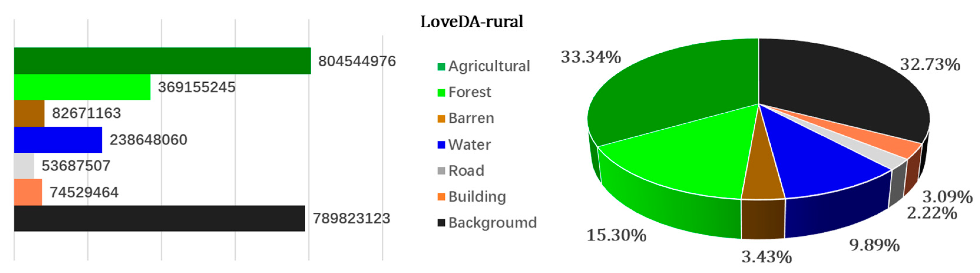
2.1. The LoveDA Dataset

The LoveDA dataset, released in 2021 by the RSIDEA team at the State Key Laboratory of Information Engineering in Surveying, Mapping, and Remote Sensing, Wuhan University, is suitable for semantic segmentation and migration learning tasks and it contains a total of 5987 urban and rural images with a spatial resolution of 0.3 $\mathrm{m}$ from three cities, Nanjing, Changzhou, and Wuhan, including seven categories: buildings, roads, water bodies, wastelands, forests, agriculture, and backgrounds. In this paper, we demonstrate the effectiveness of the proposed method in unbalanced semantic segmentation by studying the rural part of the LoveDA dataset and naming these data as the LoveDA-rural dataset. The pixel statistics for each categorical sample in the LoveDA-rural dataset are shown in Figure 1. As can be seen in Figure 1, the categories building (3.09%), road (2.22%), and barren (3.43%) have a small percentage in the dataset, and they are the minimal categories in the dataset. It is also important to note that in the overall dataset there are fewer images containing buildings and barren land, accounting for the large majority in a single image. As a result, as to whether buildings and barren land are regarded as minimal catalogue or not, it depends on the number of the analyzed images including buildings and barren land. The category of roads in both the whole dataset and a single image is a very small category, as can be seen in Figure 2. In order to observe the semantic segmentation effect of the proposed method in this paper in such a category where both the overall dataset and the single images are treated as minimal classes, a dataset LoveDA-r-road based on the rural part of the data with roads as the only minimal class was created by sieving the images containing buildings and barren land in the dataset. The proportion of each category in this dataset is shown in Figure 3, in which the road category accounts for 4.66% and is the only minimal category.

2.2. Landsat-8 Forest Fire Burning Area Images

Launched to an altitude of 705 km on 11 February 2013, Landsat-8 carries the Operational Land Imager (OLI) with an image map area of 185 × 185 km, a spatial resolution of 30 m, and a temporal resolution of 16 days, using the geographic coordinate system WGS84 [43]. The OLI collects data for visible (VNIR, bands 2–4), near-infrared (NIR, band5), and two shortwave infrared portions (SWIR, bands 6–7) of the spectrum.

Table 1. Landsat-8 OLI multispectral bands.

Band	Channel	$\mathbf{Wavelength} \left(\mathsf{\mu }\mathbf{m}\right)$	Applications
1	Coastal	0.433~0.453	Active fire detection and environmental observation in coastal zones.
2	Blue	0.450~0.515	Visible light spectrum used for geographical identification.
3	Green	0.525~0.600
4	Red	0.630~0.680
5	NIR	0.845~0.885	Active fire detection and information extraction of vegetative cover.
6	SWIR1	1.560~1.660	Active fire detection, vegetation drought detection, and mineral information extraction.
7	SWIR2	2.100~2.300	Active fire detection, vegetation drought detection, mineral information extraction, and multi-temporal analysis.

[44] demonstrates the wavelengths and application ranges for each channel.

Satellite forest fire burning area images were selected along the southwest coast of the United States and northeastern Australia during 2015–2021 and they contain forty views of images containing more than sixty forest fire events. Historical fire data were obtained from the websites of The National Interagency Fire Center (NIFC) [45] and the Department of Agriculture Fisheries and Forestry (DAFF) of Australia [46]. Considering the characteristics of recent major wildfires, [47] illustrated the significant forest fire clusters along the specific coasts of the USA and Australia, especially on account of highly combustible tree crown fuel load. A schematic map of the study area and data sampling points is shown in Figure 4.

The forest fire burning area dataset from Landsat8-OLI satellite imagery includes three categories: fire, vegetation, and background. For fire detection and vegetation cover, bands 4, 5, and 6 were selected as data inputs in this study [44].

Relying on spectral data of SWIR2 and NIR, the active detection threshold method designed by [48] applies fixed threshold and image context methods when exploring the differential radiation response of the data to realize the classification of potential active fire pixels. With this method of annotating data, we generate segmentation masks automatically based on three conditions:

Equation (1) is the threshold formula, used to identify the unambiguous fire pixels, and Equation (2) characterizes the candidate fire pixels due to the digital number (DN) folding of channel 7 (SWIR2):

$${\rho }_6>0.8 AND {\rho }_1<0.2 AND ({\rho }_5>0.4 OR {\rho }_7<0.1),$$

(1)

$$R_{75}>1.8 AND {\rho }_7-{\rho }_5>0.17 AND {\rho }_7>0.5,$$

(2)

In the above equation, ${\rho }_i$ represents the reflectance of channel $i$, and $R_{ij}$ represents the reflectance ratio of channel $i$ to $j$. Following this nomenclature, ${\rho }_1$ is the costal band centered at a wavelength of 0.443 $\mu \mathrm{m}$, ${\rho }_5$ is the NIR band centered at a wavelength of 0.865 $\mu \mathrm{m}$, while ${\rho }_6$ and ${\rho }_7$ are two SWIR bands centered at 1.610 $\mu \mathrm{m}$ and 2.190 $\mu \mathrm{m}$, respectively. The spatial resolution of all these bands is 30 $\mathrm{m}$.

All pixels must satisfy the following set of fixed thresholds and contextual tests in order to be classified as potential fire-affected pixels:

$$\{\begin{array}{c}{R}_{75}>\overline{R_{75}}+\max \left[3{\sigma }_{R_{75}}, 0.8\right]\\ {\rho }_7>\overline{{\rho }_{75}}+max\left[3{\sigma }_{{\rho }_7}, 0.08\right],\\ R_{76}>1.6\end{array}$$

(3)

Using the effective background pixels in a 61 × 61 window centered on the candidate pixels, the $\overline{R_{ij}}$ and ${\sigma }_{R_{ij}}$(${\sigma }_{{\rho }_i}$) in Equation (3), respectively, represent the mean and standard deviation calculated by the channel reflectance.

Vegetation labels are determined by the (NDVI):

$$NDVI=\frac{NIR-R}{NIR+R}>0.05,$$

(4)

When pro-processing remote sensing images, the FLAASH atmospheric-correction module and the radiometric calibration were used. The original image was cropped using a sliding frame with a step size of 256 and a size of 512 × 512. Due to the rotation invariance of the remote sensing images, only the symmetric method was used to expand the dataset. Finally, 2024 images of size 512 × 512 were obtained, and the comparison of the number of pixels in each category in the dataset is shown in Figure 5.

3. Methods

3.1. Effective Sample Space

Boundary effects emerge during the expansion of the imbalanced datasets, which means that when the number of samples in some categories increases beyond a specific number range, the model’s classification performance of that category will not be enhanced. The index of range is defined as the effective sample space that can be calculated as the following [40]:

$$E_a=\frac{\left(1-{\beta }^a\right)}{1-\beta },$$

(5)

where $a$ is the number of samples and the hyperparameter $\beta$ is the probability of overlap between the new sample and the existing sample, defined as the following:

$$\beta =\frac{N-1}{N},$$

(6)

$N$ is the size of the sample space, and as the ideal sample space is infinite, $\beta$ cannot be calculated and only the hyperparameters are taken. To calculate the hyperparameter $\beta$, the effective sample space size $E_n$ can be obtained by expanding the above equation:

$$E_n=\frac{1-{\beta }^n}{1-\beta }=1+\beta +{\beta }^2+\cdots +{\beta }^{n-1},$$

(7)

If the sum of the first $m$ terms is ${10}^p$ times the sum of the second $n-m$ terms, the second $n-m$ terms can be ignored and the value range of $p$ should be $p\ge 3$. The inequality can be listed as follows:

$$\frac{1+\beta +{\beta }^2+\cdots +{\beta }^{m-1}}{{\beta }^m+{\beta }^{m+1}+\cdots +{\beta }^{n-1}}\ge {10}^p,$$

(8)

The above inequality is equal to the following:

$$0<\beta \le \sqrt[m]{\frac{1}{{10}^p+1}},$$

(9)

The range values of the effective sample subspace can be expressed by the following inequality:

$$1<E_m\le \left(1-\frac{1}{{10}^p+1}\right)*\left(\frac{1}{1-\beta }\right),$$

(10)

The size of the effective sample subspace varies with the values of $m$ and $p$, as shown in Figure 6. The graph shows that $E_m$ has a positive correlation with $m$ and a negative correlation with $p$.

$$E_{m_{max}}=\frac{1000}{1001}*\frac{1}{1-\beta },$$

(11)

The above formula shows that for each class of samples, the probability, $\beta$, and the effective sample space size, $E_m$, corresponding to the subspace can be calculated if the number of samples in the subspace, $m$, is known. When $p$ takes the minimum value, there exists a maximum effective sample subspace. Since the datasets used in deep learning methods are all subspaces in the sample space, the effective sample subspace can be calculated.

For the parameter $\beta$, the Equation (5) is applied to the ideal sample space in the existing effective sample theory, and three values are taken for the image classification task, 0.9, 0.99, and 0.999. It is also shown that $\beta$ with the value of 0.999 has a better effective sample space calculation result compared with the other two in large datasets [40]. The effective sample numbers calculated by the above algorithm and the algorithm in this paper are shown in Figure 7.

Ideally, the number of effective samples should grow with the number of samples, but when $\beta$ is taken as a constant, the number of effective samples calculated from this constant will finally reach an upper limit, which is not consistent with the ideal situation. Therefore, the effective sample space algorithm proposed in this paper is closer to the ideal state and is more suitable for semantic segmentation tasks with a large number of samples.

3.2. Dynamic Effective Sample Class Balance (DECB) Weighting Method

In semantic segmentation tasks, to balance the contribution of each classification of a very unbalanced dataset in the loss function, the widely used dynamic class balance weighting method (DCB) [49] defines the weights as follows:

$$W_i=1-\frac{n_i}{n_{batch}},$$

(12)

In the above equation, $n_{batch}$ is the sum of the sample sizes within a batch and $n_i$ is the sample size of class $i$ within the same batch. A single batch in the neural network training process acts as a subspace, which is determined by the batch size. The DCB method is determined by the proportion of each category in this sample subspace, and the weight of each category is negatively correlated with its proportion.

In order to increase the weight of the categories with small sample sizes in the neural network training process, this paper proposes to define a minimal class in the sample subspace defined as the following:

$$n_{i_{batch}}<E_{n_{batch}},$$

(13)

$E_{n_{batch}}$ is the size of the effective sample subspace and $n_{i_{batch}}$ is the number of samples of class $i$ in a single batch. When the number of samples in a classification is less than the effective sample space corresponding to the sample space, it is defined as a minimal class, as shown in Figure 8.

In order to highlight the minority classes in neural network training and achieve class balancing, a dynamic effective class balancing (DECB) weighting method is proposed, with weights defined as follows:

$$W_{Ei}=\{\begin{array}{c}1-\frac{E_{n{i}_{batch}}}{n_{batch}}, n_{i_{batch}}<E_{n_{batch}},\\ 1-\frac{n_{i_{batch}}}{n_{batch}}, n_{i_{batch}}\ge E_{n_{batch}}\end{array}$$

(14)

$E_{n{i}_{batch}}$ can be calculated from Equation (11) and $\beta$ is given by the following equation:

$${\beta }_{i_{batch}}=\sqrt[n_{i_{batch}}]{\frac{1}{1001}},$$

(15)

Equation (13) applies the DECB method to adjust the weights of the minority classes. Since the effective number of these classes in a batch space is less than their label frequency, the weight ratio of them can be effectively increased after using $E_{n{i}_{batch}}$ instead of $n_{i_{batch}}$.

Table 2. Examples of DECB weighting method (512 × 512 size image).

Batch Size	${\mathit{N}}_{\mathit{b}\mathit{a}\mathit{t}\mathit{c}\mathit{h}}$	$\mathit{\beta }$	${\mathit{E}}_{{\mathit{n}}_{\mathit{b}\mathit{a}\mathit{t}\mathit{c}\mathit{h}}}$	${\mathit{n}}_{{\mathit{i}}_{\mathit{b}\mathit{a}\mathit{t}\mathit{c}\mathit{h}}}$	DCB Weights	${\mathit{E}}_{\mathit{n}{\mathit{i}}_{\mathit{b}\mathit{a}\mathit{t}\mathit{c}\mathit{h}}}$	DECB Weights
4	1048576	0.9999934	151623.8390	150000	0.8569	21690.3920	0.9793
8	2097152	0.9999967	303247.1785	200000	0.9046	28920.3560	0.9862
12	3145728	0.9999978	454870.5181	400000	0.8728	57840.2134	0.9816
16	4194304	0.9999984	606493.8575	600000	0.8569	86760.0703	0.9793

shows the DCB weights and DECB weights corresponding to the minority classes for a 512 × 512 size image with four types of batch size and $n_{i_{batch}}$ is the value taken to satisfy Equation (13) for ease of observation. The DECB method assigns a greater weight to the minority class.

4. Results and Discussion

4.1. Environmental Configuration and Parameter Details

This study used the Pytorch deep learning framework and implemented code based on the corresponding Python 3.6.13, with the detailed tool configuration shown in

Table 3. Environmental configuration.

Programming Environment	Auxiliary Library	Hardware Configuration	Other Software
Python3.6.13	h5py2.10.0	CPU:[email protected] GHz	Envi5.3.1
torch1.2.0	GDAL3.0.4	GPU:NVIDIA TITAN X	ArcGIS PRO
CUDA11.6	opencv4.1.2	RAM:16 GB
cuDNN8.0.4	numpy1.17.0	Numba0.26.0

.

The ratio of the training set to the test set is 6:4, and the evaluation metrics are the average of the optimal hyperparameter combinations measured by multiple training. Some of the hyperparameters used in this paper are shown in

Table 4. Parameter details.

Name of Dataset	Number of Samples	Initial Learning Rates	Decay Rate	Batch Size	Epoch
LoveDA-rural	8884	$1.50\times {10}^{-4}$	0.96	8	120
LoveDA-r-road	1571	$2.50\times {10}^{-4}$	0.96	12	150
Forest fire burning area	2022	$2.00\times {10}^{-4}$	0.96	4	150

.

4.2. Network Structure and Loss Function

The underlying neural network architecture in this paper is based on U-Net [25], which has been shown to have better results in the forest fire burning area semantic segmentation task [44]. U-Net is a fully convolutional network with two symmetric halves; the first has pooling operations that decrease the data resolution and the second has upsampling operations that restore the data to its original resolution. The first half extracts basic features and context, and the second half allows for a precise pixel-level localization of each feature, with skip connections between the two halves being used to combine the features from shallow layers with more abstract features from deeper layers [50]. The U-Net structure in this paper takes a 512*512 three-channel image as an input, and successively convolves to a feature layer depth of 1024 in the encoder part. Then, four feature layers of different sizes from the process of encoding are superimposed with the upsampling results obtained in the decoder part, and finally, the segmented image is obtained by 1*1 convolution. The network structure is shown in Figure 9. In order to verify the applicability of the weighting approach on different network architectures, two network architectures, vgg [51] and Resnet50 [52], were used as backbones, respectively, for experiments in the encoder of the U-Net network.

Softmax cross entropy (CE) and Focal loss are chosen as the weighted functions in this paper. As the most used loss function in the classification, CE loss is based on the theory that cross entropy can be used to measure the difference between the probability distribution learned by the model and the true probability distribution. Focal loss modifies the CE loss function by adding a focusing factor $\gamma$ to reduce the contribution of easily categorized samples in the loss calculation to solve the category imbalance problem. In this study, the focusing factor $\gamma$ is a constant, $\gamma =3$.

CE loss and Focal loss are defined as follows:

$$C{E}_{softmax}\left(z,y\right)=-log\left(\frac{\exp \left(z_y\right)}{{\sum }_{j=1}^n\exp \left(z_j\right)}\right),$$

(16)

$$Focal\left(z,y\right)=-{\sum }_{i=1}^C{\left(1-p_i^t\right)}^{\gamma }\log \left(p_i^t\right),$$

(17)

where $i$ and $j$ in Equations (16) and (17) represent the different categories, $z$ is the output value of each classification prediction, and $y$ is the corresponding label.

The equation for the loss function, weighted by the dynamic effective class balance according to Equation (13), is shown below:

$$DEC{B}_{softmax}\left(z,y\right)=-\left(1-\frac{E_{n_J}}{n_{batch}}\right)log\left(\frac{\exp \left(z_y\right)}{{\sum }_{j=1}^n\exp \left(z_j\right)}\right),$$

(18)

$$DEC{B}_{focal}\left(z,y\right)=-\left(1-\frac{E_{n_J}}{n_{batch}}\right)\sum _{i=1}^C{\left(1-p_i^t\right)}^{\gamma }\log \left(p_i^t\right),$$

(19)

4.3. Evaluation Metrics

The Intersection-Over-Union (IoU) metric [53], known as the Jaccard index, is widely used to evaluate segmentation performance. In forest fire burning area segmentation tasks, false negatives are more fatal than false positives. Therefore,$\mathrm{I}\mathrm{o}\mathrm{U}$, $F_1$-score [54], precision ($P$), and recall ($R$) are also used in the evaluation of segmentation results.

Since the balance between categories is an important part of this study, in order to reveal how the balance relationship between categories is affected by the modified weighting methods, specific indicators need to be calculated for each category in addition to the overall average. $F_1$-score, precision, and recall are defined as follows:

$$R=\frac{TP}{TP+FN},$$

(20)

$$P=\frac{TP}{TP+FP},$$

(21)

$$F_1=\frac{2}{1/P+1/R},$$

(22)

where $FP$, $TP$, and $FN$ are, respectively, the number of false positives, true positives, and false negatives in the segmentation results. $\mathrm{I}\mathrm{o}\mathrm{U}$, the ratio of the intersection to the union between the predict section and the true section, is defined as follows:

$$\mathrm{I}\mathrm{o}\mathrm{U}=\frac{TP}{TP+FN+FP},$$

(23)

$\mathrm{m}\mathrm{I}\mathrm{o}\mathrm{U}$ is defined as follows:

$$\mathrm{m}\mathrm{I}\mathrm{o}\mathrm{U}=\frac{1}{N}{\sum }_{i=1}^N\mathrm{I}\mathrm{o}{\mathrm{U}}_i,$$

(24)

where $N$ is the number of categories and $\mathrm{I}\mathrm{o}{\mathrm{U}}_i$ is the $\mathrm{IoU}$ score of categories $i$.

4.4. Results in the Loveda Dataset

The results of the evaluation in the LoveDA-rural dataset are shown in

Table 5. The IoU results in LoveDA-rural (%).

Backbone	Loss-Function	Background	Building	Road	Water	Barren	Forest	Agricultural	Average
vgg-16	DECB- Focal	55.89	68.06	62.74	73.59	46.92	72.51	73.35	64.72
vgg-16	DCB-Focal	56.11	67.18	61.00	73.69	47.02	73.01	73.24	64.46
resnet-50	DECB- Focal	56.46	66.1	61.00	73.85	47.96	73.15	73.9	64.63
resnet-50	DCB-Focal	57.03	65.07	60.27	74.69	48.03	73.18	74.24	64.64

.

As the two minimum categories in the LoveDA-rural dataset, IoU with DECB improved by 1% compared to DCB, which led to the increase in mIoU, but the IoU of the barren and the other majority categories declined. Furthermore, the vgg-16 network combined with Focal outperformed Resnet-50 in this dataset, and the vgg-16 network based on DECB achieved the best results in both the two smallest categories and mean metrics.

In the LoveDA-r-road dataset, the weighting methods outperformed the combination with CE over the combination with Focal by weighting object, while Resnet-50 outperformed vgg in terms of network structure. However, across all combinations of network structures and weighted objects, the evaluation indicators obtained by the DECB method are improved in most classifications, with only some decreases in forest and agricultural. In line with expectations, the very small category, road, received the largest increase of about 1.3%.

The results of the evaluation in the LoveDA-rural dataset are shown in

Table 6. The IoU results in LoveDA-r-road (%).

Backbone	Loss-Function	Background	Road	Water	Forest	Agricultural	Average
vgg-16	DECB-Focal	53.26	68.79	70.89	66.52	72.75	66.44
vgg-16	DCB-Focal	51.64	66.94	70.26	66.19	72.65	65.54
resnet-50	DECB-Focal	52.94	68.88	71.06	66.94	73.33	66.63
resnet-50	DCB-Focal	51.86	67.83	71.01	66.41	73.23	66.07
vgg-16	DECB-CE	55.1	69.79	70.85	66.82	72.98	67.11
vgg-16	DCB-CE	54.08	68.67	70.19	67.52	72.93	66.68
resnet-50	DECB-CE	55.66	68.99	71.38	66.79	73.06	67.18
resnet-50	DCB-CE	54.97	67.42	71.01	67.41	73.66	66.89

.

An example of image segmentation in the LoveDA-r-road dataset is shown in Figure 10. In Figure 10a, the gray roads occupy a smaller area than the water, agricultural land, and background. For this category, the Focal function performs less well than CE for the main road segmentation, but the DECB method can improve and optimize the original segmentation results in both network structures. The misrepresentation of woodland in the segmentation results based on the vgg can be found by visual interpretation, which may have resulted from the omission in the original labels.

The same omission may also be found in Figure 10b. The visual interpretation that the original labels are incomplete for the road sections around the lake can be found. After weighting the road category features by the DECB method, the vgg-DECB-Focal combination completely segmented the road along the lake, and for another very small category in the image, it also more accurately segmented the labelled woodland on the right side of the image and the unlabeled suspected woodland on the opposite side of the lake. These segmentation results show that the DECB method has improved the segmentation of multiple minimal categories in highly unbalanced images.

In the LoveDA-r-road dataset, DECB not only optimizes the known minimum class segmentation results, as shown in Figure 10a, but it also enables more accurate segmentation of missing annotation in images based on the learned minimum class features, as shown in Figure 10b.

The superiority of the DECB method is demonstrated by the fact that in both of the LoveDA unbalanced datasets, the DECB method is able to improve the IoU of the minimal classes with a small enhancement to the overall segmentation effect, about 0.5% of the IoU. The segmentation effect of the minority classes is enhanced by the dynamic algorithm of multi-classification balance, which finally achieves the enhancement of the overall segmentation effect of the dataset.

The DECB method can be applied to a variety of network structures, and the IoU results in the LoveDA-r-road dataset when combined with the Focal loss are shown in

Table 7. The IoU results for different networks in LoveDA-r-road (%).

Network	Weighting Methods	Background	Road	Water	Forest	Agricultural	Average
vgg-16	DECB	53.26	68.79	70.89	66.52	72.75	66.44
	DCB	51.64	66.94	70.26	66.19	72.65	65.54
Resnet-50	DECB	52.94	68.88	71.06	66.94	73.33	66.63
	DCB	51.86	67.83	71.01	66.41	73.23	66.07
PSPNet	DECB	50.78	60.69	69.61	65.41	72.96	63.90
	DCB	48.12	58.99	67.20	62.32	72.34	61.80
DeeplabV3	DECB	50.23	60.66	64.10	62.30	72.63	61.99
	DCB	46.96	60.07	62.94	62.90	71.91	60.96

.

Compared with the DCB method, the DECB method improves not only the IoU per classification but also the average IoU in a vast number of cases.

The comparison results of two segmentation methods based on multiple network structures are shown in Figure 11. After applying the DECB method, the segmentation effect of the road as a minority class in the image becomes clearer than before.

4.5. Results in the Forest Fire Burning Area Dataset

The results of the evaluation in the forest fire burning area dataset are shown in

Table 8. Results of the evaluation of the forest fire burning area dataset (%).

Backbone	Loss-Function	Fire				Vegetation				Background
		IoU	Recall	Precision	F1-Score	IoU	Recall	Precision	F1-Score	IoU	Recall	Precision
vgg-16	DECB-Focal	21.36	51.96	26.62	35.21	93.51	97.13	96.17	96.65	78.06	88.36	87.01
vgg-16	DCB-Focal	17.96	19.57	35.26	25.17	93.34	97.22	95.91	96.56	77.23	87.9	86.42
resnet-50	DECB-Focal	20.72	46.77	27.11	34.32	92.55	95.18	97.1	96.13	74.12	81.3	89.36
resnet-50	DCB-Focal	15.59	19.57	43.63	27.02	92.83	97.2	95.38	96.28	75.32	88.15	83.81
vgg-16	DECB-CE	13.14	17.51	34.46	23.22	95.2	97.47	97.61	97.54	85.95	93.97	90.97
vgg-16	DCB-CE	12.23	15.76	35.31	21.79	94.65	97.91	96.6	97.25	84.58	92.06	91.24
resnet-50	DECB-CE	18.09	27.37	34.8	30.64	94.81	97.41	97.27	97.34	84.27	94.22	88.86
resnet-50	DCB-CE	15.72	21.53	36.81	27.17	94.7	97.78	96.78	97.28	84.22	93.2	89.74

. In the forest fire burning area dataset, vgg is more advantageous than Resnet-50, while Focal performs best in the minority classes and CE performs best in the majority classes. However, the DECB method is superior to DCB in most categories, with an average increase of 3.5% in IoU for the very small categories when combined with Focal. While the above segmentation improvement is achieved, the overall segmentation of the image has an average improvement of about 1%, which does not decrease with the use of the DECB method. Furthermore, in the context of forest fire burning area segmentation tasks, where recall is more demanding, DECB in combination with Focal gives a significant increase of about 25% in this metric.

A comparison of the metrics for each combination of scenarios for forest fire burning area segmentation is shown in Figure 12. The vgg-DECB-Focal combination achieves the highest IoU, recall, and F1-score scores of all the combinations, indicating that this combination performs better in terms of semantic segmentation, avoiding false negatives, and balancing false negatives and false positives. The Resnet-DCB-CE combination outperforms in the precision metric, which is due to the average outweighing of CE over Focal, DCB over DECB, and Resnet over vgg in this metric, but is also inferior to the other three.

Two examples of the segmentation results in the forest fire burning area dataset are shown in Figure 13. In Figure 13a, the segmentation results of the large burning area can be divided into three combinations: the first one is based on the Resnet network structure. These combinations have better segmentation results for forest fire burning areas without smoke obscuration but they cannot segment the smoke-obscured forest fire pixels. Of these combinations, the best segmentation results come from the DECB method of weighting. The second is the three vgg combinations other than DECB-vgg, and none of them can achieve many segmentations of forest fire pixels inside and outside the smoke area, and the results obtained are a little fragmented. The third is the vgg-DECB-Focal method. This combination segmented many forest fire pixels to form a relatively ideal forest fire burning area, sacrificing the segmentation effect of the background class, but achieving the objective of highlighting the segmented forest fire pixels required for the task.

The segmentation results of the small burning area in Figure 13b can be divided into two categories, with the first seven combinations performing the segmentation task relatively well in the smoke-obscured small burning area. Especially of these seven combinations, vgg-DECB-CE achieves a better job of segmenting the tiny fire spots. With the addition of Focal to further highlight the very small class, the vgg-DECB-Focal method shows much more false positives and such results are clearly unsatisfactory.

According to Figure 13, the DECB method can improve the model’s focus on forest fire pixels to a certain extent, and it is particularly effective when dealing with smoke-obscured forest fire burning areas; although, there exists the possibility of overtraining, making the false positive rate increase in the absence of smoke obscuration. Therefore, in order to obtain the best segmentation results, the most suitable combination of the network structure–loss function weighting methods should be adopted.

5. Conclusions

The image segmentation results based on deep learning are greatly affected by the existence of highly unbalanced data among various categories in the remote sensing dataset. To solve this problem, the following recommendations are made in this paper: Firstly, the corresponding datasets are established, including a tri-classified, extremely unbalanced forest fire burning area segmentation dataset and two highly unbalanced segmentation datasets from a publicly available dataset. Secondly, a method for computing effective samples in the semantic segmentation task and a weighting method for dynamic effective class balancing are proposed to solve the class imbalance problem in multi-category semantic segmentation. Finally, the effectiveness and robustness of the method are verified experimentally.

The results show that the DECB method can improve minority class segmentation in the semantic segmentation task by combining Focal_loss and CE in a U-Net network architecture with vgg and Resnet-50 as different encoders, respectively. In the publicly available LoveDA-rural and LoveDA-r-road datasets, the average IOU of very small class segmentation results increased by approximately 1%, and the overall average cross-merge ratio also increased due to changes in class balance. In the forest fire burning area dataset, the maximum increase in the mean IOU for forest fire pixel segmentation was about 4%, and the recall increased by approximately 20%, which is more advantageous in the forest fire burning area segmentation task. Meanwhile, the DECB method proposed in this paper can effectively improve the segmentation effect of the minimum classes without sacrificing overall accuracy. Meanwhile, the DECB method proposed in this paper can effectively improve the segmentation effect of the minimum classes without sacrificing overall accuracy.

However, there are still some issues that need to be addressed in further research. The quantitative imbalance relationship between the various categories in a single image or a single batch is not exactly consistent with the dataset itself, which is the fundamental reason why the data in the sample space cannot be distributed as evenly as ideal.

References

1. Barmpoutis, P.; Papaioannou, P.; Dimitropoulos, K.; Grammalidis, N. A Review on Early Forest Fire Detection Systems Using Optical Remote Sensing. Sensors 2020, 20, 6442. [Google Scholar] [CrossRef]
2. Johnston, J.; Paugam, R.; Whitman, E.; Schiks, T.; Cantin, A. Remote Sensing of Fire Behavior. Encyclopedia of Wildfire and Wildland-Urban Interface (WUI) Fires; Springer: Berlin/Heidelberg, Germany, 2019. [Google Scholar]
3. Ghahreman, R.; Rahimzadegan, M. Calculating net radiation of freshwater reservoir to estimate spatial distribution of evaporation using satellite images. J. Hydrol. 2022, 605, 127392. [Google Scholar] [CrossRef]
4. Brinkerhoff, C.B.; Gleason, C.J.; Zappa, C.J.; Raymond, P.A.; Harlan, M.E. Remotely Sensing River Greenhouse Gas Exchange Velocity Using the SWOT Satellite. Glob. Biogeochem. Cycles 2022, 36, e2022GB007419. [Google Scholar] [CrossRef]
5. Weng, F.; Yu, X.; Duan, Y.; Yang, J.; Wang, J. Advanced Radiative Transfer Modeling System (ARMS): A New-Generation Satellite Observation Operator Developed for Numerical Weather Prediction and Remote Sensing Applications. Adv. Atmos. Sci. 2020, 37, 3–8. [Google Scholar] [CrossRef] [Green Version]
6. Brown, A.; Ferentinos, K. Exploring the Potential of Sentinels-1 & 2 of the Copernicus Mission in Support of Rapid and Cost-effective Wildfire Assessment. Int. J. Appl. Earth Obs. Geoinf. 2018, 73, 262–276. [Google Scholar]
7. Kotaridis, I.; Lazaridou, M. Remote sensing image segmentation advances: A meta-analysis. ISPRS J. Photogramm. Remote Sens. 2021, 173, 309–322. [Google Scholar] [CrossRef]
8. Guo, X.; Chen, Y.; Liu, X.; Zhao, Y. Extraction of snow cover from high-resolution remote sensing imagery using deep learning on a small dataset. Remote Sens. Lett. 2020, 11, 66–75. [Google Scholar] [CrossRef]
9. Cheng, G.; Han, J. A Survey on Object Detection in Optical Remote Sensing Images. ISPRS J. Photogramm. Remote Sens. 2016, 117, 11–28. [Google Scholar] [CrossRef] [Green Version]
10. Thenkabail, P. Remotely Sensed Data Characterization, Classification, and Accuracies; CRC Press: Boca Raton, FL, USA, 2015. [Google Scholar]
11. Cheng, H.D.; Jiang, X.H.; Sun, Y.; Wang, J. Color image segmentation: Advances and prospects. Pattern Recognit. 2001, 34, 2259–2281. [Google Scholar] [CrossRef]
12. Derivaux, S.; Lefèvre, S.; Wemmert, C.; Korczak, J. Watershed Segmentation of Remotely Sensed Images Based on a Supervised Fuzzy Pixel Classification. In Proceedings of the IEEE International Geosciences and Remote Sensing Symposium (IGARSS), Denver, CO, USA, 31 July–4 August 2006. [Google Scholar] [CrossRef] [Green Version]
13. Blaschke, T.; Lang, S.; Lorup, E.; Strobl, J.; Zeil, P. Object-Oriented Image Processing in an Integrated GIS/Remote Sensing Environment and Perspectives for Environmental Applications. Environ. Inf. Plan. Politics Public 2000, 2, 555–570. [Google Scholar]
14. Blaschke, T.; Burnett, C.; Pekkarinen, A. Image Segmentation Methods for Object-based Analysis and Classification. Remote Sensing Image Analysis: Including the Spatial Domain; Springer: Berlin/Heidelberg, Germany, 2004; pp. 211–236. [Google Scholar]
15. Navulur, K. Multispectral Image Analysis Using the Object-Oriented Paradigm; CRC Press: Boca Raton, FL, USA, 2006; pp. 1–155. [Google Scholar]
16. Felzenszwalb, P.F.; Huttenlocher, D.P. Efficient Graph-Based Image Segmentation. Int. J. Comput. Vis. 2004, 59, 167–181. [Google Scholar] [CrossRef]
17. Alshehhi, R.; Marpu, P.R. Hierarchical graph-based segmentation for extracting road networks from high-resolution satellite images. ISPRS J. Photogramm. Remote Sens. 2017, 126, 245–260. [Google Scholar] [CrossRef]
18. Wang, Y.; Meng, Q.; Qi, Q.; Yang, J.; Ying, L. Region Merging Considering Within- and Between-Segment Heterogeneity: An Improved Hybrid Remote-Sensing Image Segmentation Method. Remote Sens. 2018, 10, 781. [Google Scholar] [CrossRef] [Green Version]
19. Shelhamer, E.; Long, J.; Darrell, T. Fully Convolutional Networks for Semantic Segmentation. IEEE Trans. Pattern Anal. Mach. Intell. 2017, 39, 640–651. [Google Scholar] [CrossRef]
20. Chen, L.C.; Papandreou, G.; Kokkinos, I.; Murphy, K.; Yuille, A.L. Semantic Image Segmentation with Deep Convolutional Nets and Fully Connected CRFs. In Proceedings of the International Conference on Learning Representations, Banff, AB, Canada, 14–16 April 2014. [Google Scholar]
21. Chen, L.C.; Papandreou, G.; Kokkinos, I.; Murphy, K.; Yuille, A.L. DeepLab: Semantic Image Segmentation with Deep Convolutional Nets, Atrous Convolution, and Fully Connected CRFs. IEEE Trans. Pattern Anal. Mach. Intell. 2018, 40, 834–848. [Google Scholar] [CrossRef] [PubMed] [Green Version]
22. Chen, L.-C.; Papandreou, G.; Schroff, F.; Adam, H. Rethinking Atrous Convolution for Semantic Image Segmentation. arXiv 2017, arXiv:1706.05587. [Google Scholar]
23. Chen, L.-C.; Zhu, Y.; Papandreou, G.; Schroff, F.; Adam, H. Encoder-Decoder with Atrous Separable Convolution for Semantic Image Segmentation. In Proceedings of the Computer Vision—ECCV 2018, Munich, Germany, 8–14 September 2018; pp. 833–851. [Google Scholar]
24. Zhao, H.; Shi, J.; Qi, X.; Wang, X.; Jia, J. Pyramid Scene Parsing Network. In Proceedings of the 2017 IEEE Conference on Computer Vision and Pattern Recognition (CVPR), Honolulu, HI, USA, 21–26 July 2017; pp. 6230–6239. [Google Scholar]
25. Ronneberger, O.; Fischer, P.; Brox, T. U-Net: Convolutional Networks for Biomedical Image Segmentation. In Proceedings of the Medical Image Computing and Computer-Assisted Intervention—MICCAI 2015, Munich, Germany, 5–9 October 2015; pp. 234–241. [Google Scholar]
26. Yan, Z.; Su, Y.; Sun, H.; Yu, H.; Ma, W.; Chi, H.; Cao, H.; Chang, Q. SegNet-based left ventricular MRI segmentation for the diagnosis of cardiac hypertrophy and myocardial infarction. Comput. Methods Programs Biomed. 2022, 227, 107197. [Google Scholar] [CrossRef] [PubMed]
27. Xia, W.; Ma, C.; Liu, J.; Liu, S.; Chen, F.; Zhi, Y.; Duan, J. High-Resolution Remote Sensing Imagery Classification of Imbalanced Data Using Multistage Sampling Method and Deep Neural Networks. Remote Sens. 2019, 11, 2523. [Google Scholar] [CrossRef] [Green Version]
28. Diakogiannis, F.I.; Waldner, F.; Caccetta, P.; Wu, C. ResUNet-a: A deep learning framework for semantic segmentation of remotely sensed data. ISPRS J. Photogramm. Remote Sens. 2020, 162, 94–114. [Google Scholar] [CrossRef] [Green Version]
29. Feng, W.; Huang, W.; Ye, H.; Zhao, L. Synthetic Minority Over-Sampling Technique Based Rotation Forest for the Classification of Unbalanced Hyperspectral Data. In Proceedings of the IGARSS 2018–2018 IEEE International Geoscience and Remote Sensing Symposium, Valencia, Spain, 22–27 July 2018; pp. 2651–2654. [Google Scholar]
30. Zhang, Y.; Kang, B.; Hooi, B.; Yan, S.; Feng, J. Deep Long-Tailed Learning: A Survey. arXiv 2021, arXiv:2110.04596. [Google Scholar]
31. Aggarwal, U.; Popescu, A.; Hudelot, C. Minority Class Oriented Active Learning for Imbalanced Datasets. In Proceedings of the 2020 25th International Conference on Pattern Recognition (ICPR), Milano, Italy, 10–15 January 2021; pp. 9920–9927. [Google Scholar]
32. Zhang, C.; Pan, T.-Y.; Chen, T.; Zhong, J.; Fu, W.; Chao, W.-L. Learning with Free Object Segments for Long-Tailed Instance Segmentation. In Proceedings of the Computer Vision–ECCV 2022: 17th European Conference, Tel Aviv, Israel, 23–27 October 2022. [Google Scholar]
33. Buda, M.; Maki, A.; Mazurowski, M. A systematic study of the class imbalance problem in convolutional neural networks. Neural Netw. 2017, 106, 249–259. [Google Scholar] [CrossRef] [Green Version]
34. He, H.; Garcia, E.A. Learning from Imbalanced Data. IEEE Trans. Knowl. Data Eng. 2009, 21, 1263–1284. [Google Scholar] [CrossRef]
35. Park, S.; Lim, J.; Jeon, Y.; Choi, J.Y. Influence-Balanced Loss for Imbalanced Visual Classification. In Proceedings of the 2021 IEEE/CVF International Conference on Computer Vision (ICCV), Montreal, QC, Canada, 10–17 October 2021; pp. 715–724. [Google Scholar]
36. Zhang, S.; Li, Z.; Yan, S.; He, X.; Sun, J. Distribution Alignment: A Unified Framework for Long-tail Visual Recognition. In Proceedings of the 2021 IEEE/CVF Conference on Computer Vision and Pattern Recognition (CVPR), Nashville, TN, USA, 20–25 June 2021; pp. 2361–2370. [Google Scholar]
37. Ren, J.; Yu, C.; Sheng, S.; Ma, X.; Zhao, H.; Yi, S.; Li, H. Balanced meta-softmax for long-tailed visual recognition. In Proceedings of the 34th International Conference on Neural Information Processing Systems, Vancouver, BC, Canada, 7–8 June 2020; p. 351. [Google Scholar]
38. Shu, J.; Xie, Q.; Yi, L.; Zhao, Q.; Zhou, S.; Xu, Z.; Meng, D. Meta-weight-net: Learning an explicit mapping for sample weighting. In Proceedings of the 33rd International Conference on Neural Information Processing Systems, Vancouver, BC, Canada, 8–14 December 2019; p. 172. [Google Scholar]
39. Hossain, M.S.; Betts, J.M.; Paplinski, A.P. Dual Focal Loss to address class imbalance in semantic segmentation. Neurocomputing 2021, 462, 69–87. [Google Scholar] [CrossRef]
40. Cui, Y.; Jia, M.; Lin, T.Y.; Song, Y.; Belongie, S. Class-Balanced Loss Based on Effective Number of Samples. In Proceedings of the 2019 IEEE/CVF Conference on Computer Vision and Pattern Recognition (CVPR), Long Beach, CA, USA, 15–20 June 2019; pp. 9260–9269. [Google Scholar]
41. Lin, T.Y.; Goyal, P.; Girshick, R.; He, K.; Dollár, P. Focal Loss for Dense Object Detection. IEEE Trans. Pattern Anal. Mach. Intell. 2017, 42, 2999–3007. [Google Scholar]
42. Wang, J.; Zheng, Z.; Ma, A.; Lu, X.; Zhong, Y. LoveDA: A Remote Sensing Land-Cover Dataset for Domain Adaptive Semantic Segmentation. arXiv 2021, arXiv:2110.08733. [Google Scholar]
43. USGS. US Geological Survey. Available online: https://www.usgs.gov/landsat-missions/landsat-8 (accessed on 1 March 2022).
44. Wang, Z.; Yang, P.; Liang, H.; Zheng, C.; Yin, J.; Tian, Y.; Cui, W. Semantic Segmentation and Analysis on Sensitive Parameters of Forest Fire Smoke Using Smoke-Unet and Landsat-8 Imagery. Remote Sens. 2022, 14, 45. [Google Scholar] [CrossRef]
45. NIFC. National Interagency Fire Center. Available online: https://www.nifc.gov/ (accessed on 1 October 2020).
46. DAFF. Department of Agriculture Fisheries and Forestry. Available online: https://www.agriculture.gov.au/ (accessed on 1 October 2020).
47. Kganyago, M.; Shikwambana, L. Assessment of the characteristics of recent major wildfires in the USA, Australia and Brazil in 2018–2019 using multi-source satellite products. Remote Sens. 2020, 12, 1803. [Google Scholar] [CrossRef]
48. Schroeder, W.; Oliva, P.; Giglio, L.; Quayle, B.; Lorenz, E.; Morelli, F. Active fire detection using Landsat-8/OLI data. Remote Sens. Environ. 2016, 185, 210–220. [Google Scholar] [CrossRef] [Green Version]
49. Lu, S.; Gao, F.; Piao, C.; Ma, Y. Dynamic Weighted Cross Entropy for Semantic Segmentation with Extremely Imbalanced Data. In Proceedings of the 2019 International Conference on Artificial Intelligence and Advanced Manufacturing (AIAM), Dublin, Ireland, 16–18 October 2019; pp. 230–233. [Google Scholar]
50. De Almeida Pereira, G.H.; Fusioka, A.M.; Nassu, B.T.; Minetto, R. Active fire detection in Landsat-8 imagery: A large-scale dataset and a deep-learning study. ISPRS J. Photogramm. Remote Sens. 2021, 178, 171–186. [Google Scholar] [CrossRef]
51. Simonyan, K.; Zisserman, A. Very Deep Convolutional Networks for Large-Scale Image Recognition. arXiv 2014, arXiv:1409.1556. [Google Scholar]
52. He, K.; Zhang, X.; Ren, S.; Sun, J. Deep Residual Learning for Image Recognition. In Proceedings of the IEEE Conference on Computer Vision and Pattern Recognition (CVPR), Las Vegas, NV, USA, 27–30 June 2016; pp. 770–778. [Google Scholar]
53. Pinheiro, P.O.; Collobert, R.; Dollár, P. Learning to segment object candidates. In Proceedings of the 28th International Conference on Neural Information Processing Systems—Volume 2, Montreal, Canada, 7–12 December 2015; pp. 1990–1998. [Google Scholar]
54. Chinchor, N.A.; Sundheim, B.M. MUC-5 evaluation metrics. In Proceedings of the Fifth Message Understanding Conference (MUC-5), Baltimore, MD, USA, 25–27 August 1993. [Google Scholar]
Figure 1. Number and percentage of pixels in each classification sample in the LoveDA-rural dataset.
Remotesensing 15 01768 g001
Figure 2. The minimal classes sample of the LoveDA dataset: (a) barren; (b) building; and (c) road.
Remotesensing 15 01768 g002
Figure 3. Number and percentage of pixels in each classification sample in the LoveDA-r-road dataset.
Remotesensing 15 01768 g003
Figure 4. Schematic map of the study area: (a) Australia, and (b) the west coast of the United States and Canada.
Remotesensing 15 01768 g004aRemotesensing 15 01768 g004b
Figure 5. Number and percentage of pixels in each classification sample in the forest fire burning area dataset.
Remotesensing 15 01768 g005
Figure 6. Scatterplot (a) and the fitted surfaces (b) of the effective sample subspace values E m with the values of m ( 0 < m 11500 ) and p ( 3 p 25 ).
Remotesensing 15 01768 g006
Figure 7. Comparison between the original effective sample algorithm and the algorithm in this paper ( β n e w ).
Remotesensing 15 01768 g007
Figure 8. N b a t c h is a subspace of the sample space N . Within this subspace, the category with a larger sample space than E n b a t c h is the majority class, otherwise it is the minority class.
Remotesensing 15 01768 g008
Figure 9. Schematic of the U-Net network structure with the vgg structure in the encoder section.
Remotesensing 15 01768 g009
Figure 10. Example of segmentation results for the LoveDA-r-road dataset: (a) Sample of correct triple classification markers and their segmentation results. (b) Sample of incorrect triple classification markers and their segmentation results.
Remotesensing 15 01768 g010
Figure 11. Example of segmentation results for multiple network structures in the LoveDA-r-road dataset: (a) example 1 and (b) example 2.
Remotesensing 15 01768 g011
Figure 12. Comparison chart of condition combinations and evaluation indicators for forest fire burning area segmentation results corresponding evaluation indicators.
Remotesensing 15 01768 g012
Figure 13. Example of segmentation results for the forest fire burning area dataset: (a) sample of the large burning area, and (b) sample of the small burning area.
Remotesensing 15 01768 g013