Photometric Catalogue for Space and Ground Night-Time Remote-Sensing Calibration: RGB Synthetic Photometry from Gaia DR3 Spectrophotometry

Abstract

Recent works have made strong efforts to produce standardised photometry in RGB bands. For this purpose, we carefully defined the transmissivity curves of RGB bands and defined a set of standard sources using the photometric information present in Gaia EDR3. This work aims not only to significantly increase the number and accuracy of RGB standards but also to provide, for the first time, reliable uncertainty estimates using the BP and RP spectrophotometry published in Gaia DR3 instead of their integrated photometry to predict RGB photometry. Furthermore, this method allows including calibrated sources regardless of how they are affected by extinction, which was a major shortcoming of previous work. The RGB photometry is synthesised from the Gaia BP and RP low-resolution spectra by directly using their set of coefficients multiplied with some basis functions provided in the Gaia catalogue for all sources published in Gaia DR3. The output synthetic magnitudes are compared with the previous catalogue of RGB standards available.

1. Introduction

RGB photometry has been increasingly used in recent decades for amateur and professional astronomical studies due to the high-quality and economically accessible digital cameras. In recent works [1,2], a strong effort was made to produce a standardised system for RGB photometry to enhance the quality of the studies to be performed with these kind of devices. This is relevant not only for ground measurements but also for satellite observations as stars are also being used to calibrate night-time remote-sensing platforms, such as the images taken from the International Space Station (ISS) [3] and the Suomi North Polar Partnership and NOAA-20, Visible Infrared Imaging Radiometer Suite Day Night Band (VIIRS) [4,5].

Ref. [1] defined the transmissivity passbands for RGB filters derived from 28 different types of cameras analysed by [6]. Ref. [1] also established standardised synthetic RGB photometry for a set of 1346 bright stars belonging to the Bright Star Catalogue [7]. This small set of standards was expanded in number (about 15 million sources) by [2] (hereafter, C21) using photometric transformations derived from integrated photometry in Gaia EDR3 [8,9]. This work aims to further expand the quality and number of sources in the sky with known RGB photometry that could be used as standards. For that purpose, we use synthetic photometry derived from the Gaia DR3 low-resolution spectra [10,11,12].

In Gaia DR3 [13], a set of 220 million sources were released together with their blue (BP) and red (RP) low-resolution spectra. When compared with RGB passbands (Figure 1), we can see that RGB passbands mostly cover only the wavelength range covered by BP instrument (In order to avoid confusion, specifically with the G band, in this paper, we used $G_{\mathrm{Gaia}}$, $G_{\mathrm{BP}}$ and $G_{\mathrm{RP}}$ to refer to Gaia magnitudes and $R_{\mathrm{RGB}}$, $G_{\mathrm{RGB}}$ and $B_{\mathrm{RGB}}$ for magnitudes in the RGB system.).

It is known [11,12,14] that the BP instrument has more calibration issues present than RP. Fortunately, most of these issues are assigned to difficulties in the ultraviolet region ($\lambda <400$ nm), where the Gaia response decreases abruptly, and the amount of standards with enough flux in that range diminishes substantially. As none of the RGB passbands extends to so short wavelengths, we can still use Gaia spectrophotometry to derive synthetic RGB photometry from them.

We describe, in Section 2, the methodology used to derive the synthetic photometry from Gaia spectrophometry, producing the synthetic photometry for all sources with BP and RP spectra (hereafter, XP is used to refer to BP or RP spectra indistinctly) present in Gaia DR3 and not flagged as variable in the catalogue. In Section 3, we compare the samples of sources in this work with the ones used by C21, comparing also the RGB magnitudes obtained in both studies. In Section 4, we study the validity of the polynomials defined in C21 for those sources in Gaia DR3 without XP spectra available. Section 5 explains how to access the final catalogue of RGB magnitudes created in this work (in form of an online table and through a Python code called rgbloom. Finally, we present a brief summary of the results and conclusions of this work in Section 6.

2. RGB Catalogue Construction

Gaia [15] is a survey mission, which allows homogeneously observing all sources in the sky up to magnitude 21. In addition to the 3D positions, motions and broad band photometry, Gaia also provides spectrophotometry for 219 million sources [10,11,12]. The astrophysical information contained in these spectra allows the study of the physical properties of the observed sources to analyse, for instance, their spectral features as performed in [16].

The homogeneity of the spectrophotometry over all sky positions also makes Gaia a suitable mission to be used as a reference to establish a catalogue of standard sources in any photometric system covering the optical range. This possibility to derive synthetic photometry from the Gaia spectrophotometry has been previously explored by several works [11,14,17,18]. We use here the same methodology (briefly described in the following paragraphs) to derive the synthetic photometry in RGB bands from XP Gaia DR3 spectrophotometry. Notice that, as recommended by [11], we do not use, in this work, the sampled spectra to derive the synthetic photometry; instead, we directly work with the source coefficients to obtain our estimations of the RGB magnitudes.

From the externally calibrated Gaia mean spectra, $f_s\left(\lambda \right)$, for a given source, s, we can derive its synthetic integrated flux ($F_{sj}$) in a given passband, j, with transmissivity equal to $T_j\left(\lambda \right)$ by deriving the following integral expression with wavelength $\lambda$:

$$F_{sj}=\frac{\int f_s\left(\lambda \right)·T_j\left(\lambda \right)·\lambda d\lambda }{\int T_j\left(\lambda \right)·\left(\frac{c}{\lambda }\right)d\lambda },$$

(1)

where the ABMAG system is considered for the zeropoint [19,20,21] with c as the speed of light.

The Gaia externally calibrated mean spectra $f_s\left(\lambda \right)$ is described as the weighted sum of the BP and RP contributions, $f_s^{\mathrm{BP}}\left(\lambda \right)$ and $f_s^{\mathrm{RP}}\left(\lambda \right)$, respectively:

$$f_s\left(\lambda \right)=w^{\mathrm{BP}}\left(\lambda \right)·f_s^{\mathrm{BP}}\left(\lambda \right)+w^{\mathrm{RP}}\left(\lambda \right)·f_s^{\mathrm{RP}}\left(\lambda \right),$$

(2)

with $w^{\mathrm{BP}}\left(\lambda \right)$ and $w^{\mathrm{RP}}\left(\lambda \right)$ as their weighted contributions to the total flux of each wavelength from the XP instruments.

In its turn, $f_s^{\mathrm{BP}}\left(\lambda \right)$ and $f_s^{\mathrm{RP}}\left(\lambda \right)$ are described as a set of N coefficients, $b_{sn}$, multiplied by a set of basis functions, ${\phi }_n$:

$$f_s^{\mathrm{XP}}\left(\lambda \right)=\sum _{n=1}^N{b}_{sn}^{\mathrm{XP}}·{\phi }_n^{\mathrm{XP}}\left(\lambda \right),$$

(3)

The set of basis functions, ${\phi }_n^{\mathrm{XP}}\left(\lambda \right)$, and weights, $w^{\mathrm{XP}}\left(\lambda \right)$, were published together with Gaia DR3 and are available on this webpage: https://www.cosmos.esa.int/web/gaia/dr3-xpmergexpsampling, accessed on 12 July 2022.

Combining Equations (1)–(3), we can derive the synthetic flux, $F_{sj}$, in a given passband j as:

$$\begin{array}{ccc}\hfill F_{sj}& =& {\displaystyle \sum _{n=1}^N}{b}_{sn}^{\mathrm{BP}}·\left(\frac{\int w^{BP}\left(\lambda \right)·{\phi }_n^{\mathrm{BP}}\left(\lambda \right)·T_j\left(\lambda \right)·\lambda d\lambda }{\int T_j\left(\lambda \right)·\left(\frac{c}{\lambda }\right)d\lambda }\right)+\hfill \\ & +& {\displaystyle \sum _{n=1}^N}{b}_{sn}^{\mathrm{RP}}·\left(\frac{\int w^{RP}\left(\lambda \right)·{\phi }_n^{\mathrm{RP}}\left(\lambda \right)·T_j\left(\lambda \right)·\lambda d\lambda }{\int T_j\left(\lambda \right)·\left(\frac{c}{\lambda }\right)d\lambda }\right)\equiv \hfill \\ & \equiv & {\displaystyle \sum _{n=1}^N}{b}_{sn}^{\mathrm{BP}}·X_{nj}^{\mathrm{BP}}+{\displaystyle \sum _{n=1}^N}{b}_{sn}^{\mathrm{RP}}·X_{nj}^{\mathrm{RP}},\hfill \end{array}$$

(4)

where the $X_{nj}^{\mathrm{XP}}$ terms do not depend on the source and can be derived and stored previously for any passbands and then applied to any required source using their $b_{sn}^{\mathrm{XP}}$ coefficients without the need to recompute $X_n^{\mathrm{XP}}$ terms again.

These integrated fluxes can be also expressed in terms of ABMAG system magnitudes, $m_{sj}$, by using the flux in that passband measured for an input flux of $3.631\times {10}^{-23}$ W/Hz/m². We name that flux as ${\mathrm{ZP}}_j$. Thus, the magnitude can be expressed as:

$$m_{sj}=-2.5log\left(\frac{F_{sj}}{{\mathrm{ZP}}_j}\right).$$

(5)

From the covariance matrix, $C_{nm}^{\mathrm{XP}}$, assigned to the source coefficients, we can also derive the uncertainty in the derived magnitudes as:

$${\sigma }_{sj}=\sqrt{A_j^{\mathrm{BP}}+A_j^{\mathrm{RP}}},$$

(6)

where $A_j^{\mathrm{XP}}$ can be derived using:

$$A_j^{\mathrm{XP}}=\sum _{n=1}^N{X}_{nj}^{\mathrm{XP}}·\left(\sum _{m=1}^N{C}_{nm}^{\mathrm{XP}}·X_{mj}^{\mathrm{XP}}\right).$$

(7)

Gaia DR3 published a total of 219,197,643 sources (see De Angeli et al. [11]) with XP continuous spectra. From these, a total of 6,093,025 sources have the flag phot_variable_flag=’VARIABLE’. We show the variable sources subtracted from the sample in colour-magnitude diagrams (Figure 2) as well as their $G_{\mathrm{Gaia}}$ and $G_{\mathrm{BP}}-G_{\mathrm{RP}}$ histograms (Figure 3).

These variable sources cannot be considered here for our purposes of establishing a set of reliable RGB standards. We also aimed to select only sources with phot_variable_flag= ’CONSTANT’; however, no sources with Gaia DR3 XP spectra have this flag value, as only sources with phot_variable_flag=’NOT_AVAILABLE’ and ’VARIABLE’ are present in the catalogue. This is because Gaia DR3 is still an intermediate release and because the mission has not yet finished to be completely sure that a given source is really constant. Future Gaia releases could identify some sources finally included in the catalogue as variables when considering a larger time interval covering the full mission.

Although other types of sources (quasars, galaxies, crowded fields, etc.) were not suitable to be used as RGB standards, we decided to keep them in the catalogue in order to allow a wider range of applications for this catalogue, and only explicit variable sources identified by the Gaia catalogue were excluded from it. With the large density of sources available in the new catalogue, a posterior outlier identification, based on statistical analysis, can be conducted in order to exclude them from the calibration procedure.

Thus, we derived the RGB synthetic magnitudes for all 213,104,618 sources with phot_variable_flag≠’VARIABLE’. After removing 40,616 sources with unreliable RGB magnitude estimates, a final sample of 213,064,002 objects was created—hereafter, the 200 M sample. In a small subsample of this collection, the RGB magnitude estimates are missing in some of the 3 bands (159,456, 14,546 and 486 objects in $B_{\mathrm{RGB}}$, $G_{\mathrm{RGB}}$ and $R_{\mathrm{RGB}}$, respectively). This is likely due to very low signal in these wavelength ranges present in the Gaia spectrophotometry. We decided to keep the affected sources because, in all these cases, a magnitude estimate is available in at least one of the RGB bands.

As the number of variable sources represents less than 3% of the total number of Gaia DR3 sources with XP data, the general plots included in [11] to describe Gaia DR3 XP data, can also be used here to describe the main characteristics of our catalogue of RGB standards. The only missing sources in our sample are the ones represented in Figure 2 and Figure 3.

3. Comparison with the C21 Sample

The new 200 M sample exhibits clear advantages over its predecessor published by C21. The most obvious advantage is the fact that the RGB magnitude estimates are directly computed from the source spectrum without the need to employ any approximate calibration, nor introducing constraints on the source colour or extinction. In this section, we provide a more detailed description of the benefits of using the new 200 M sample provided with this paper.

3.1. Number of Calibrated Sources

With this work, we move from the ∼15 million sources in C21 to more than 200 million objects. This can be easily visualized in the maps displayed in Figure 4, which represent the density of sources on the celestial sphere in Galactic coordinates (using a Mollweide projection with healpix of level 6 with a pixel size of 0.84 square degrees). Not surprisingly, the 200 M sample is concentrated towards the Galactic plane, not being affected by the scarcity of sources in the directions of high interstellar extinction as seen with the C21 sample.

The corresponding histograms of the source density are displayed in Figure 5. Panel (a) shows that, as expected, there are many directions in the celestial sphere in which the density of stars corresponding to the 200 M sample is clearly larger than as shown by the sources in the C21 sample. The zoom near the origin, panel (b), reveals that the density distribution of the C21 sample is bimodal with a first peak in the first histogram bin, corresponding to the interval $[0,10]$ objects/pixel and a second peak in the interval $[120,130]$ objects/pixel. The first peak corresponds to the directions of high extinction that are purposely excluded by C21.

The 200 M histogram is also bimodal with a first peak in the interval $[210,240]$ objects/pixel and a higher second peak in the interval $[470,480]$ sources/pixel. This reflects the selection criteria chosen to publish XP spectra for Gaia DR3 (see De Angeli et al. [11]). In both samples, the histogram distributions are clearly asymmetric as indicated by the location of their respective means (vertical dotted lines) and medians (vertical dashed lines), whose values are given in the figure caption.

Considering that the pixel size employed in the maps displayed in Figure 4 is slightly below 1 square degree, we confirm that the 200 M sample offers several hundred sources per square degree in most regions of the sky. A more detailed calculation indicates that 99.7% of the celestial sphere is covered with a source density above 100 sources/(square degree) by this catalogue. The rest of the sky with less sources present corresponds to regions in the Gaia mission with less transits and without Gaia spectrophotometry available in Gaia DR3 [11].

Clearly, the above numbers should be taken with some caution because, in a practical way, the number of usable sources will also be a function of the magnitude limit reached. In this sense, Figure 6 displays the variation in the number of sources as a function of the magnitude in the $G_{\mathrm{RGB}}$ band. The plot shows the histogram (dotted lines) and the cumulative sum (thick full lines) for the C21 (orange) and the 200 M samples (blue). In both samples, there is a sudden decrease in the number of sources for $G_{\mathrm{RGB}}\gtrsim 17.5$ mag.

This is because most of the sources published in Gaia DR3 were selected to have $G_{\mathrm{Gaia}}<17.65$ mag, although the XP spectra for some sources (including white dwarfs, galaxies and quasars) were also explicitly published above this magnitude limit (see De Angeli et al. [11]). The cumulative number of stars down to some particular $G_{\mathrm{RGB}}$ values are listed in

Table 1. Cumulative sums down to some particular $G_{\mathrm{RGB}}$ value for the C21 and the 200 M samples.

${\mathit{G}}_{\mathbf{RGB}}$ Interval [mag]	Sources in C21	Sources in 200 M
<10	133,019	299,041
<11	344,349	775,526
<12	761,279	1,948,176
<13	1,431,314	4,636,535
<14	2,484,448	10,495,506
<15	3,977,325	22,967,532
<16	6,546,925	48,355,681
<17	10,346,030	97,464,183
<18	13,820,929	182,081,668
<19	14,854,959	209,094,405
<20	14,854,959	212,129,751
≲21	14,854,959	213,064,002

. The M200 sample clearly outnumbers the C21 sample in number of sources at any magnitude value.

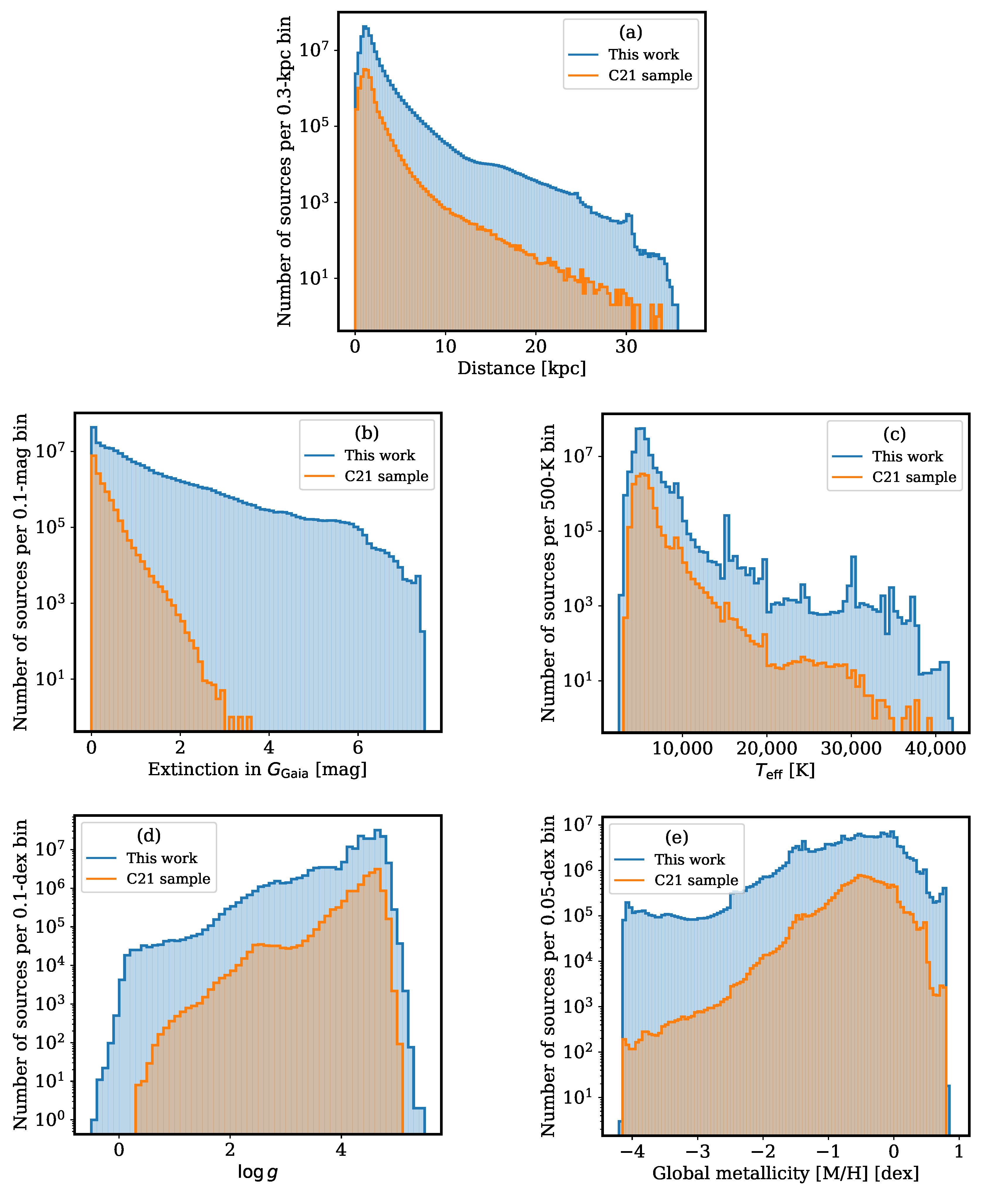
3.2. Source Characteristics

Apart from the different number of sources included in the 200 M and C21 samples, important differences in some specific characteristics of the sources are worth mentioning. In particular, the C21 subsample was restricted to sources with $-0.5\le {\mathrm{G}}_{\mathrm{BP}}-{\mathrm{G}}_{\mathrm{RP}}\le 2.0\mathrm{mag}$, whereas the 200 M sample does not include this constraint. This is clearly manifested in the histogram displayed in Figure 7, which shows that the new 200 M sample (blue filled histogram) also includes much redder objects that were not included in the C21 sample (black line).

In addition, this figure also represents the histograms corresponding to the 200 M subsamples corresponding to particular sources not classified as simple stars in Gaia DR3 (namely the sources flagged as non_single_star, in_qso_candidates and in_galaxy_candidates), for which the polynomial RGB calibration in C21, derived only for single stars, is not suitable.

We also explore, in Figure 8, the histogram distribution of some additional parameters derived from the Gaia DR3 data, in particular, the distance_gspphot (in kpc, panel (a)) and extinction in the ${\mathrm{G}}_{\mathrm{Gaia}}$ band ag_gspphot (in magnitudes, panel (b)) as well as typical stellar parameters, such as the effective temperature teff_gspphot (in K, panel (c)), surface gravity logg_gspphot (logarithm of cgs units, panel (d)) and global metallicity mh_gspphot (dex units, panel (e)). The 200 M sample contains proportionally more distant sources than does the C21 sample, although the most noticeable difference is the inclusion of more sources with much larger extinction. The 200 M catalogue incorporates proportionally more stars with large effective temperature, low surface gravity and low metallicity.

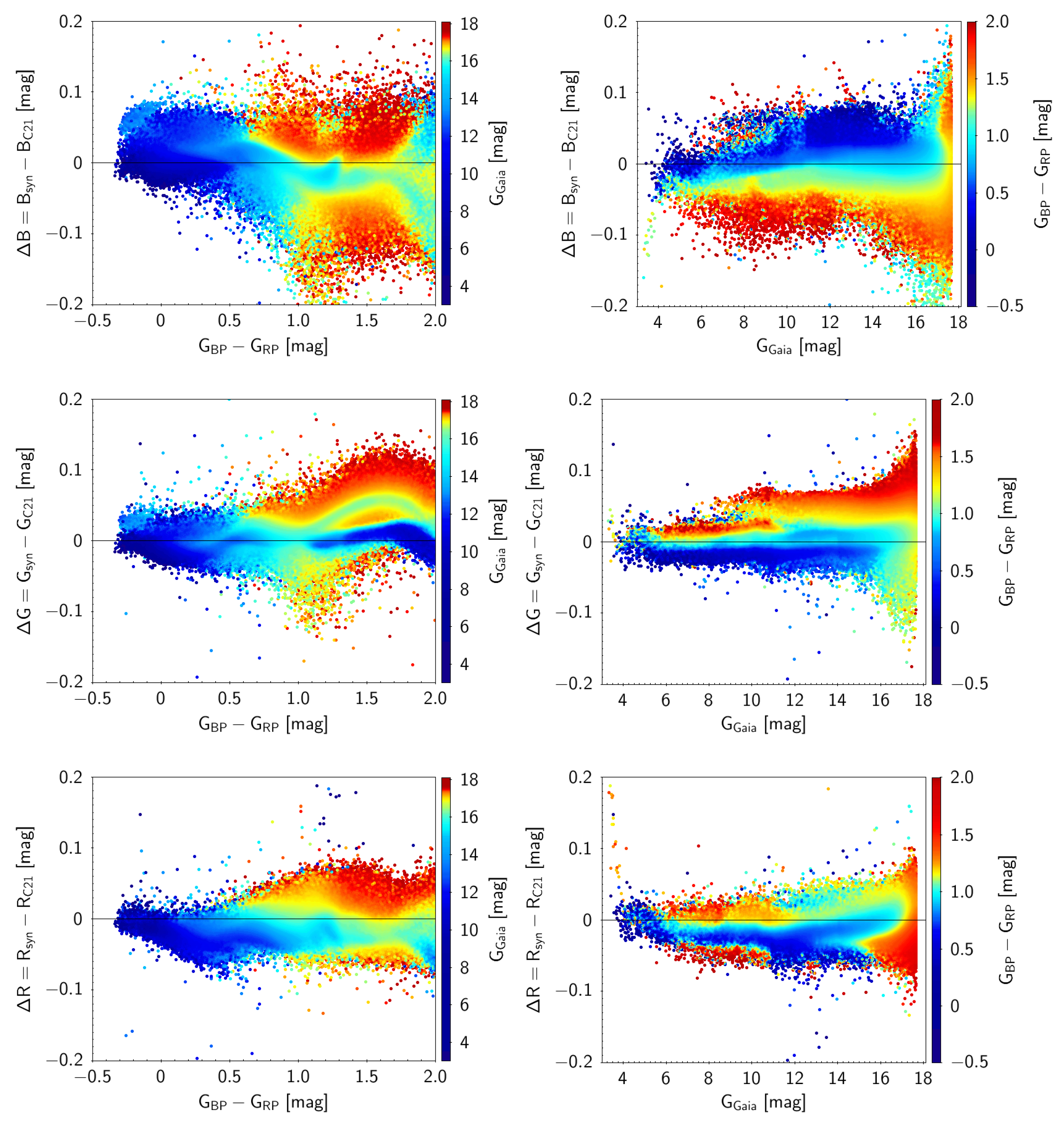
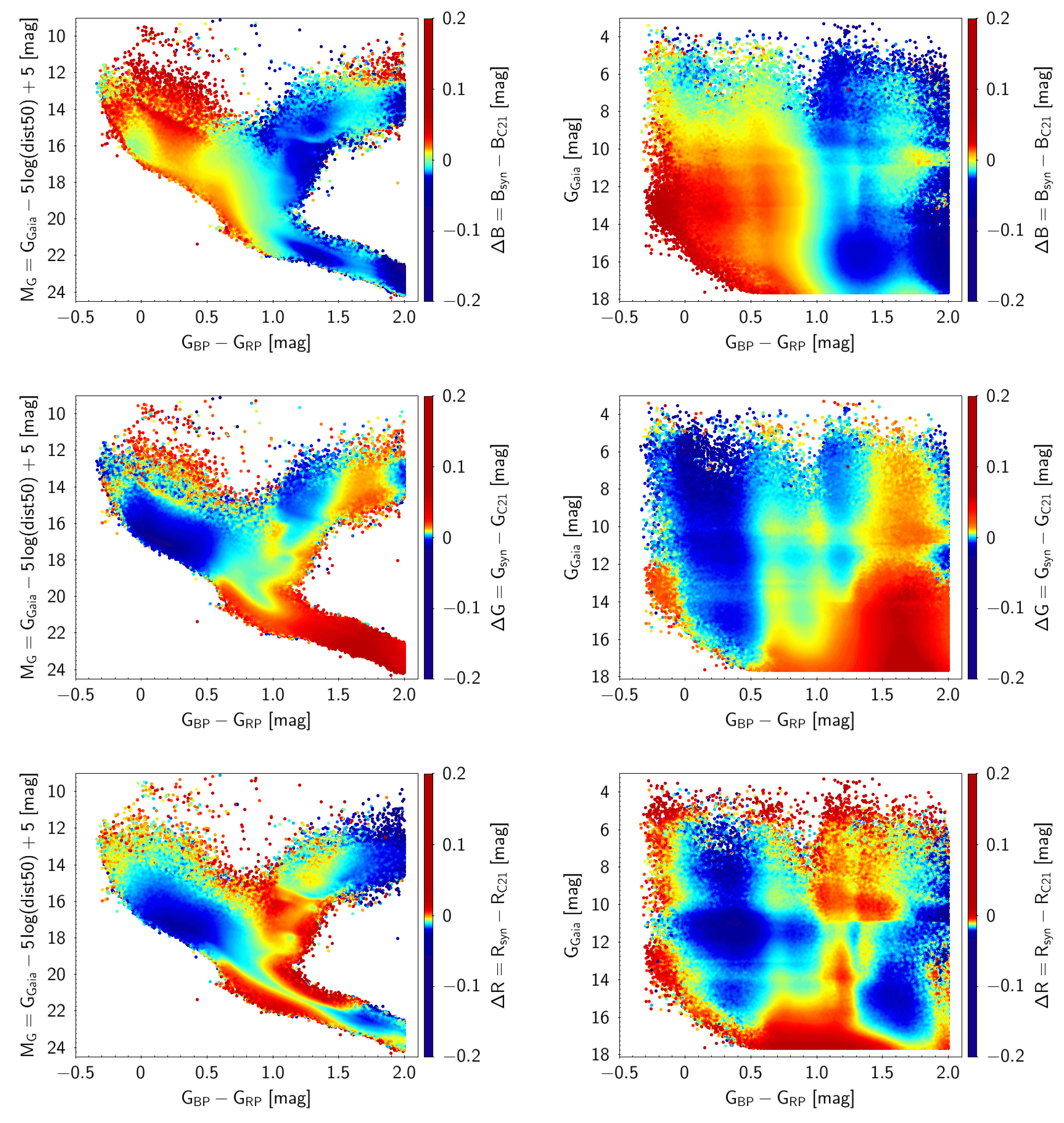
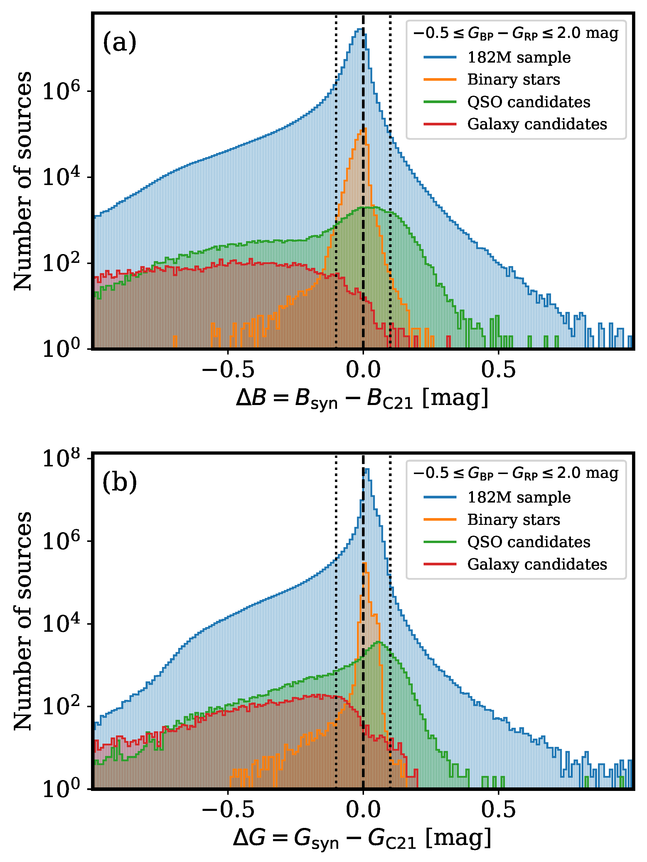
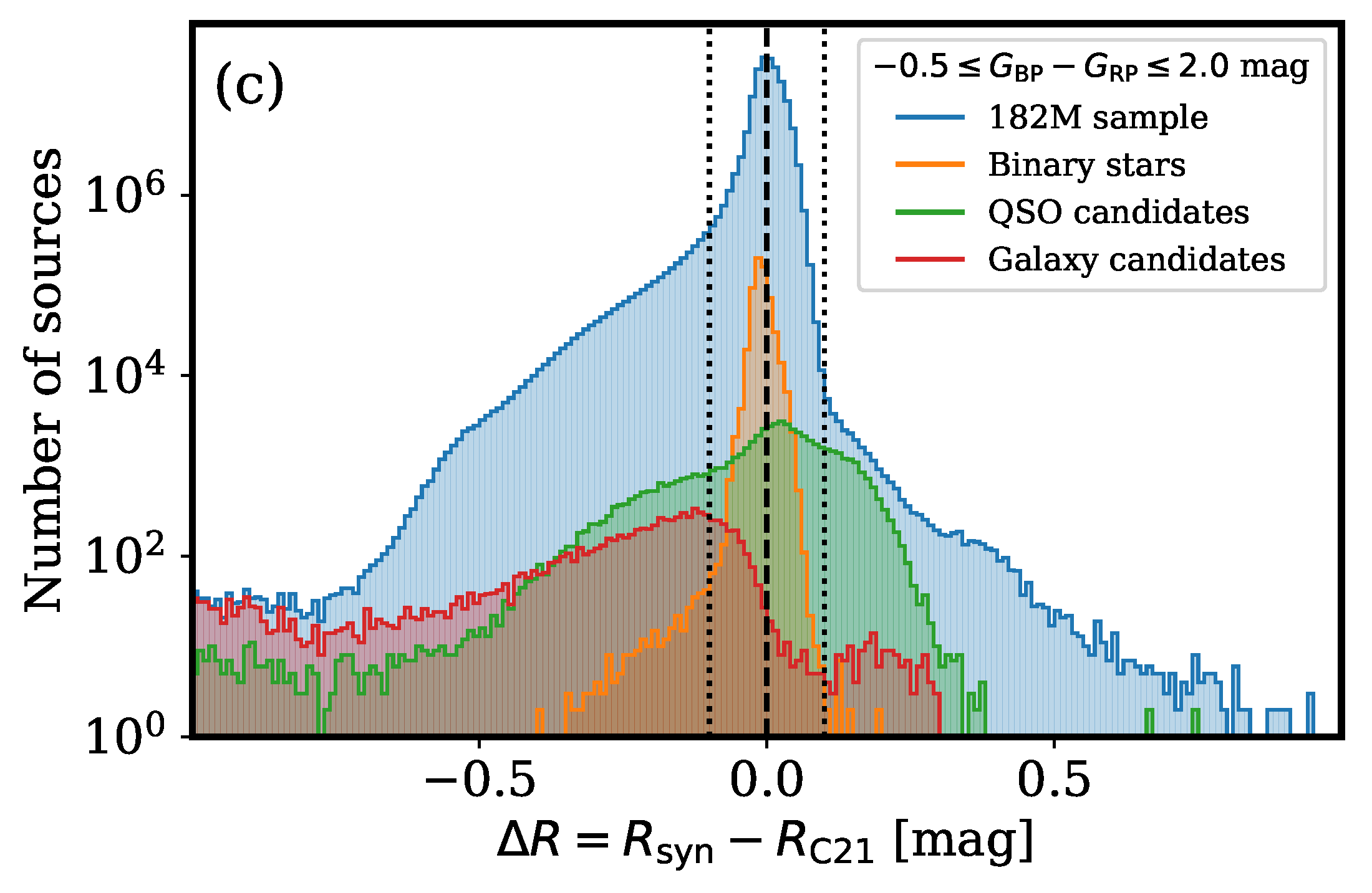
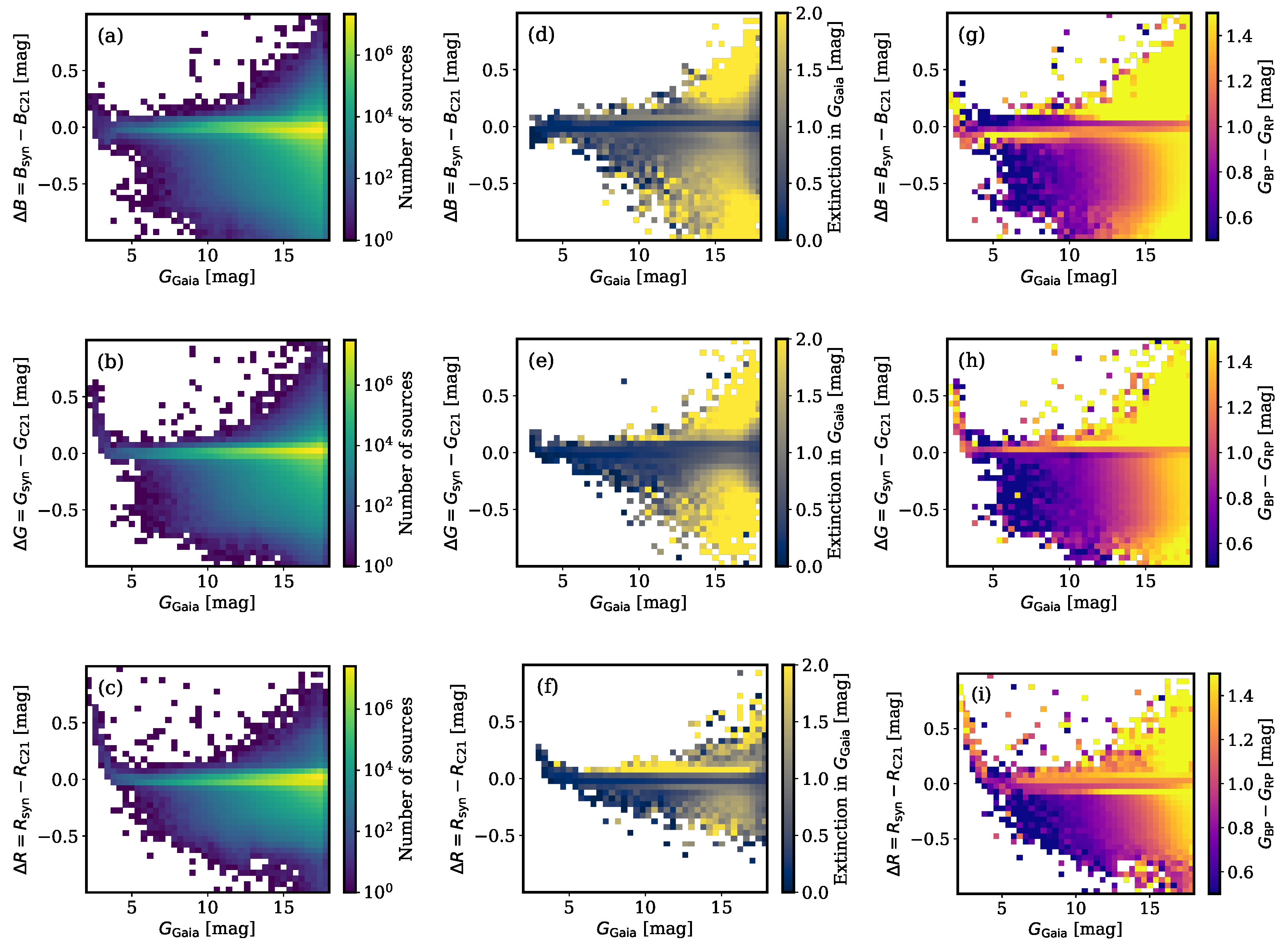
3.3. Magnitude Residuals

As the synthetic photometry in the 200 M sample is derived directly from the observed spectra and not predicted based on broad band photometry, the values obtained in this work should be more accurate than those provided by C21. Thus, the level of discrepancy should be mainly constrained by the precision of C21. We compare, in Figure 9 and Figure 10, the synthetic photometry derived here with the predictions provided by C21 for 12,920,293 non-variable sources in common. As expected, the discrepancies mostly fall in the $\pm 0.1$ mag range, which was the required accuracy claimed in C21. This provides confidence in the validity of our results.

The observed biases and colour trends in the differences shown in Figure 9 and Figure 10 are due to systematics in the Gaia spectra (see Gaia Collaboration et al. [14]) and the photometric transformations proposed by C21—being more important for the latter. The ‘bridge’ structure present in the $G_{\mathrm{RGB}}$ residual (middle-left panel in Figure 9) with $1.0<G_{\mathrm{BP}}-G_{\mathrm{RP}}<2.0$ mag contains main sequence stars, although giants have lower levels of residuals).

On the other hand, the results in the right panels of Figure 9 and Figure 10 show the different behaviour present for $G_{\mathrm{Gaia}}<11.5$ mag with respect to fainter magnitudes. This feature is likely induced by Gaia XP data as sources with $G_{\mathrm{Gaia}}<11.5$ mag are observed with different gating strategies in Gaia to avoid saturation (see [15,22]). For these bright Gaia sources, larger systematics are expected in the XP spectra due to the lower number of calibrators present for those special gating conditions used to minimise saturation events in Gaia.

The method for deriving the synthetic RGB magnitudes explained in Section 2 allows for the derivation of the associated uncertainties, and it is possible to examine their behaviour as a function of the relevant parameters. In particular, Figure 11 represents 2D histograms with the density of sources as a function of $G_{\mathrm{Gaia}}$ (the horizontal axis) and the uncertainties in the synthetic magnitudes $B_{\mathrm{RGB}}$, $G_{\mathrm{RGB}}$ and $R_{\mathrm{RGB}}$ (panels (a), (b) and (c), respectively). Not surprisingly, the uncertainties increase when moving to fainter objects. The red filled circles mark the 99th percentile at each 0.4 mag bin in the horizontal axis. Interestingly, these numbers are below 0.01 mag for a wide $G_{\mathrm{Gaia}}$ interval, increasing beyond $G_{\mathrm{Gaia}}\gtrsim 14$ mag.

Since the number of faint sources is larger than the number of bright ones, the 99th percentiles for the whole sample with values of 0.075, 0.022 and 0.019 mag for $B_{\mathrm{RGB}}$, $G_{\mathrm{RGB}}$ and $G_{\mathrm{RGB}}$, respectively, (represented with the dashed horizontal magenta line in each panel) are naturally larger than the values for bright sources (with lower uncertainties but less abundant in the total sample). It is important to highlight that, although the uncertainties are unavoidably larger for fainter objects, the also larger number of available sources at those magnitude regimes should allow the simultaneous observation of many more of them to be used as standards. The statistical combination of these measurements should help to diminish the uncertainties at the faint end.

4. Validity of the C21 Polynomial Calibration

Considering that the 200 million of sources with XP spectra in Gaia DR3 represents only 10% of the total two billion sources with available Gaia photometry, we explore here the validity of the polynomial calibrations published by C21 to estimate RGB magnitudes for the missing sources. With this aim, we applied those polynomial functions to the 200 M subsample verifying $-0.5\le G_{\mathrm{BP}}-G_{\mathrm{RP}}\le 2.0$ mag (the same constraint employed by C21) and derived the differences with the RGB estimates derived from the synthetic photometry computed in this work. The histograms of those differences are represented in Figure 12 for the $B_{\mathrm{RGB}}$, $G_{\mathrm{RGB}}$ and $R_{\mathrm{RGB}}$ bands (panels (a), (b) and (c), respectively).

Each panel represents the histogram corresponding to the full subsample after applying the colour constraint (∼182 million objects—hereafter, 182 M samples; blue filled histogram) as well as the histograms of those sources that are not classified as single stars (with the same criteria employed in Figure 7). Interestingly, 93.6%, 97.8% and 98.3% of the sources exhibit differences within the $\pm 0.1$ mag interval for $B_{\mathrm{RGB}}$, $G_{\mathrm{RGB}}$ and $R_{\mathrm{RGB}}$, respectively, (note that the vertical scale in the histograms is logarithmic). It is also evident that RGB predictions for objects flagged as in_qso_candidates and in_galaxy_candidates exhibit much larger deviations, although they have a small contribution in the total number of sources.

An expanded representation of the above results is shown in the 2D histograms displayed in Figure 13, where the magnitude differences are represented as a function of ${\mathrm{G}}_{\mathrm{Gaia}}$ with colour coding for the histograms according to the source density (first column, panels (a), (b) and (c)), extinction in $G_{\mathrm{Gaia}}$ (second column, panels (d), (e) and (f)) and $G_{\mathrm{BP}}-G_{\mathrm{RP}}$ (third column, panels (g), (h) and (i)). These histograms reveal a systematic offset for very bright sources (saturated in Gaia XP spectra; see Riello et al. [9] and De Angeli et al. [11]).

The figure also shows an expected increase in the differences of the magnitude predictions when considering fainter objects. Interstellar extinction has an important impact on the derived residuals, specifically in panels (d) and (e) for sources with $G_{\mathrm{Gaia}}>13\mathrm{mag}$. There are also some clear systematic magnitude differences depending on the source $G_{\mathrm{BP}}-G_{\mathrm{RP}}$ colour. Notwithstanding these relevant differences in the prediction of RGB magnitudes when using the C21 polynomial functions, it is important to highlight that, as previously mentioned, the predictions still fall within the $\pm 0.1\mathrm{mag}$ interval for a large fraction of the considered sources.

Thus, although the 200 M sample provides more reliable RGB predictions, the C21 calibrations may still be useful when used with the corresponding caution (i.e., avoiding high extinction regions, restricting the $G_{\mathrm{BP}}-G_{\mathrm{RP}}$ source colour and using a large number of calibrating sources in order to derive statistical averages).

5. Accessing the 200 M Sample

The 200 M sample produced in this work is accessible through an online table (

Table 2. First rows of the online table with the synthetic RGB magnitudes ($B_{\mathrm{RGB}}$, $G_{\mathrm{RGB}}$ and $R_{\mathrm{RGB}}$) and their associated uncertainties (${\sigma }_B$, ${\sigma }_G$ and ${\sigma }_R$) derived for the 200 M sample from the Gaia DR3 XP spectra for non-variable sources in the Gaia catalogue with id number equal to source_id. The column objtype is a flag that indicates the type of object in Gaia DR3: 1 for sources flagged as non_single_star, 2 for objects in in_qso_candidates, 3 for sources in in_galaxy_candidates and 0 for the rest of the sample. In addition, the last column, qlflag, provides a global quality flag, which is 0 for reliable sources and  1 for objects with any indication of potential problem (blending, contamination or non-stellar identification). The full table can be downloaded from the link provided in the text, and will also be available at the CDS.

Source_id	${\mathit{B}}_{\mathbf{RGB}}$	${\mathit{G}}_{\mathbf{RGB}}$	${\mathit{R}}_{\mathbf{RGB}}$	${\mathit{\sigma }}_{\mathit{B}}$	${\mathit{\sigma }}_{\mathit{G}}$	${\mathit{\sigma }}_{\mathit{R}}$	objtype	qlflag
4295806720	18.245	17.935	17.678	0.011	0.009	0.011	0	0
38655544960	15.003	14.570	14.171	0.003	0.002	0.002	0	0
1275606125952	16.849	16.519	16.266	0.005	0.004	0.006	0	0
1653563247744	16.544	16.336	16.196	0.005	0.004	0.005	0	0
2851858288640	12.779	12.550	12.387	0.001	0.001	0.002	0	0
3332894779520	13.335	12.894	12.539	0.002	0.001	0.002	0	0
3371550165888	15.314	14.938	14.615	0.003	0.002	0.003	0	1
3508989119232	15.736	15.431	15.199	0.003	0.003	0.003	0	0
4711579935744	14.736	14.481	14.300	0.002	0.002	0.003	0	0
4814659150336	18.490	17.854	17.297	0.013	0.009	0.009	0	1
5192616270720	18.370	17.551	16.964	0.013	0.007	0.007	0	0
5291399870976	17.301	17.033	16.842	0.006	0.005	0.007	0	0
5291399871488	18.935	18.296	17.686	0.019	0.012	0.011	0	0
·	·	·	·	·	·	·	·	·
·	·	·	·	·	·	·	·	·
·	·	·	·	·	·	·	·	·

shows the first rows of the catalogue), which is available as a large, (5.0 GB) single, compressed CSV file (available at https://nartex.fis.ucm.es/~ncl/rgbphot/gaiaDR3/RGBsynthetic_NOVARIABLES/sortida_XpContinuousMeanSpectrum_RGB_NOVARIABLES_final.csv.gz, accessed on 24 March 2023) (15 GB after decompressing). The flag $-99.0$ is employed in this table to indicate missing values in any of the RGB magnitudes or in their associated uncertainties.

As mentioned in Section 2, we have not removed the small fraction of objects in the 200 M sample classified in Gaia DR3 as belonging to one of the following categories: non_single_star (0.31% of the sample), in_qso_candidates (0.03%) and in_galaxy_candidates (0.01%). Although none of them have been thus far identified as a variable by Gaia, their use as reliable RGB calibrators should be properly checked through the statistical comparison with reliable sources located in their neighbourhood. All these sources are identified with the flag objtype in Table 2.

In addition, we also assigned a global quality flag to each source, qlflag, provided in the last column of Table 2). We define qlflag = 0 for reliable sources (74.2% of the 200 M sample) and assign qlflag = 1 for those objects suspicious of suffering any potential problem (blending, contamination or non-stellar identification; 25.8% of the sample). As expected, the uncertainties in the RGB synthetic magnitudes are larger for the qlflag = 1 sources as displayed in Figure 14.

Complementary to the online table, in order to ease access to synthetic RGB photometry, we created a Python package called rgbloom (available at https://github.com/guaix-ucm/rgbloom, accessed on 24 March 2023), which performs cone search queries around any position on the celestial sphere. This code is an updated version of rgblues (available at https://github.com/guaix-ucm/rgblues, accessed on 24 March 2023), the tool created by C21 to retrieve RGB magnitudes from the 15 M sample.

Once installed, the code can be easily executed from the command line—for example, using a command like this one:

$ rgbloom 56.66 24.10 1.0 12

The four numerical arguments correspond to the position search values (RA, DEC and search radius) in decimal degrees and the limiting $G_{\mathrm{Gaia}}$ magnitude. In the example command shown here, we are searching for sources brighter that $G_{\mathrm{Gaia}}=12$ mag within a circular aperture of radius 1 degree with centre at right ascension RA = 56.66 deg and declination DEC = 24.10 deg (corresponding to the Pleiades star cluster).

The steps followed by rgbloom to provide its output are the following:

1.

Cone search in Gaia DR3 down to the pre-defined limiting $G_{\mathrm{Gaia}}$ magnitude, retrieving the following parameters: source_id, ra, dec, phot_g_mean_mag, phot_bp_mean_mag, phot_rp_mean_mag and phot_variable_flag.

2.

Initial RGB magnitude estimation using the polynomial transformations given in Equations (2)–(4) by C21.

3.

Retrieval of the RGB synthetic magnitudes for sources in the 200 M sample within the healpix level-8 tables enclosing the region of the sky defined in the initial cone search.

4.

Cross-matching between the Gaia DR3 and the 200 M subsamples to identify sources with RGB synthetic magnitudes estimated from the XP low-resolution spectra.

5.

Generation of the output files. In particular, two files (in CSV format) are generated: rgbloom_200m.csv, which contains the sources belonging to the 200 M sample with RGB synthetic magnitudes; and rgbloom_no200m.csv, which includes sources that do not belong to the 200 M sample. In this latter case, the RGB magnitudes provided in the file correspond to the estimates derived using the polynomial relationships in C21. It is important to remember (see Section 3) that these estimates are more uncertain than the new RGB values computed in this work and that they can be biased due to systematic effects introduced by interstellar extinction by exhibiting a colour outside the $-0.5\le G_{\mathrm{BP}}-G_{\mathrm{RP}}\le 2.0$ interval (where the C21 calibrations were computed) or by variability of the source.

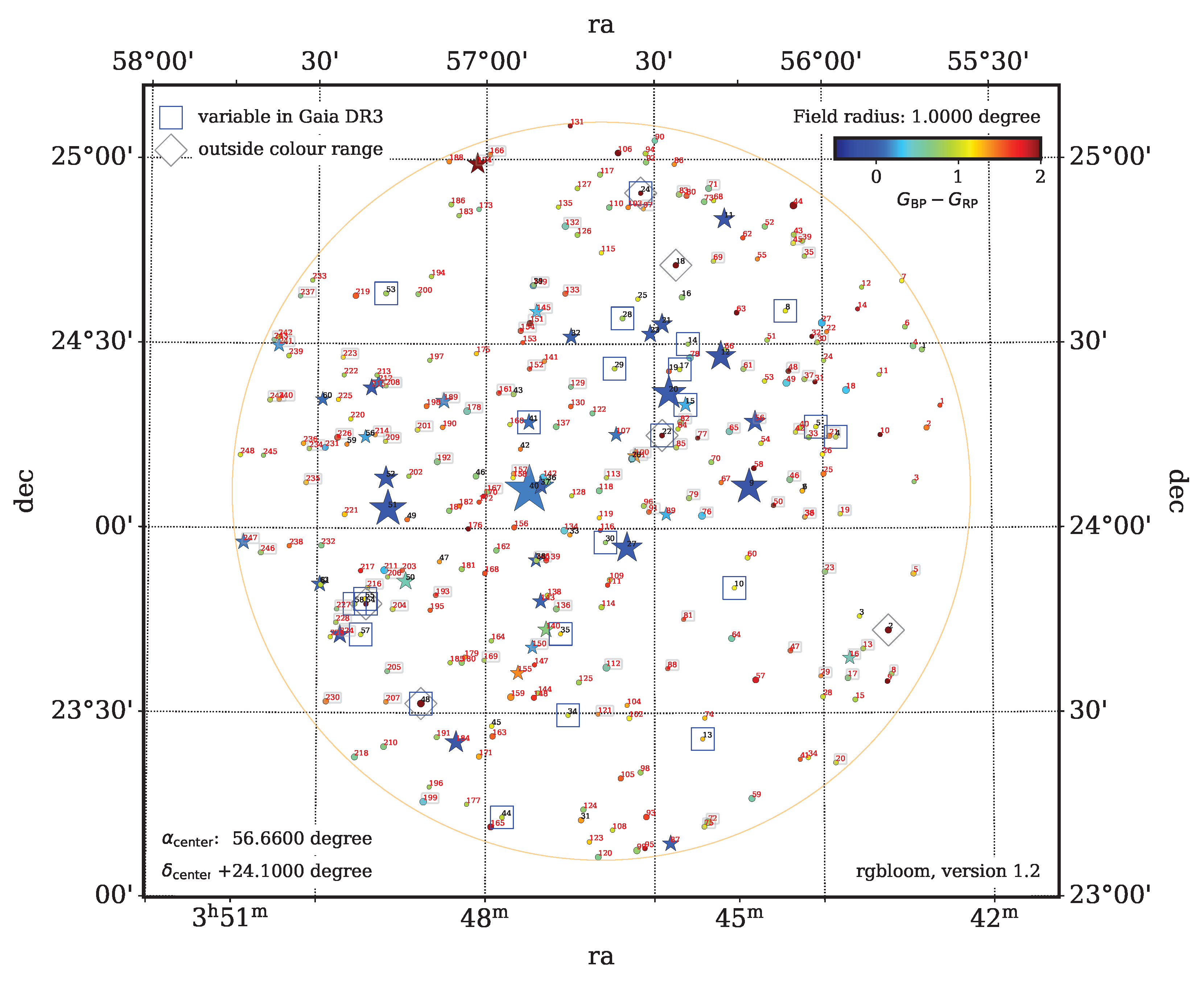
6.

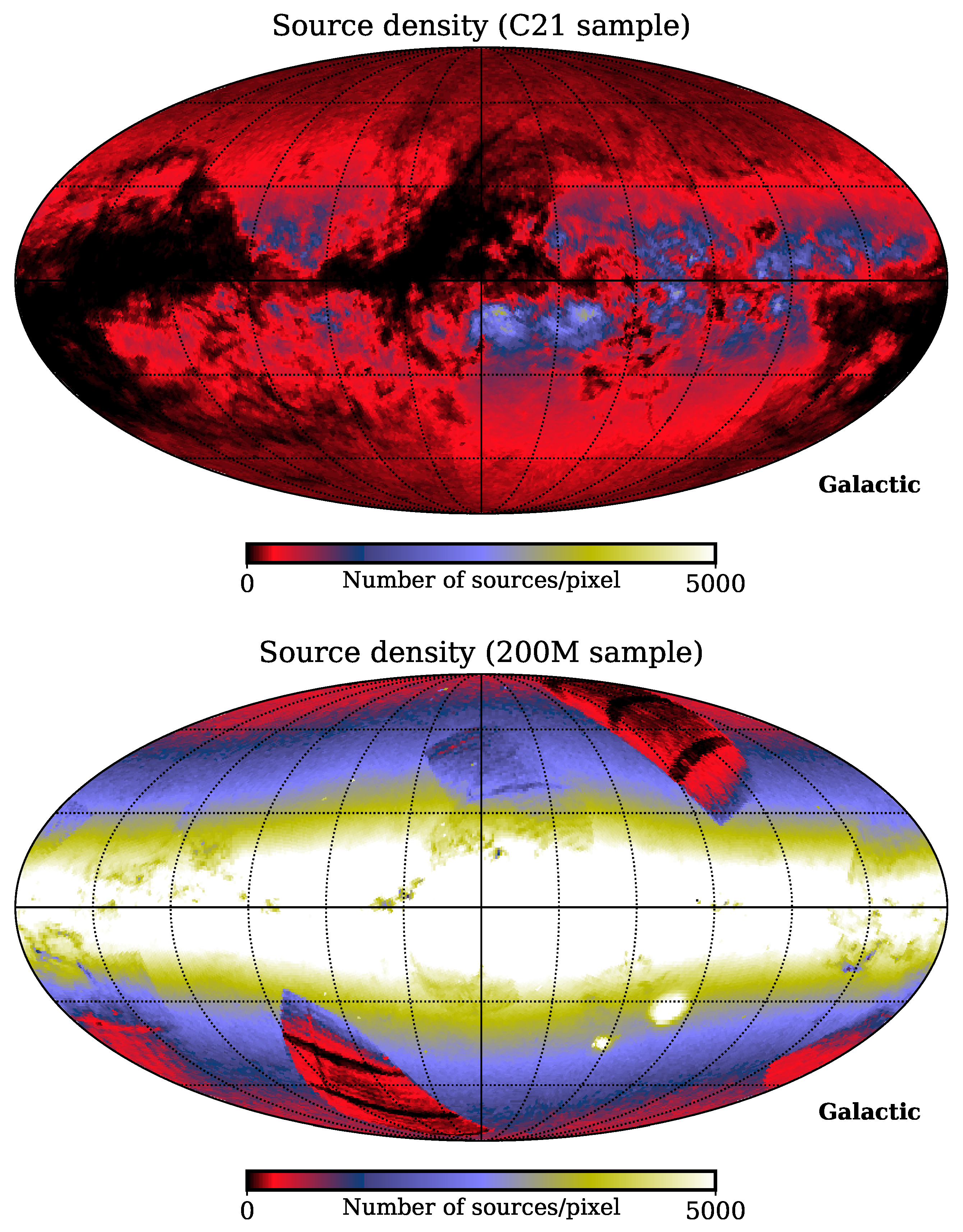
Creation of a finding chart of the results (see the example in Figure 15 for the region around the Pleiades star cluster). The users of rgbloom should rely more strongly on the RGB estimates corresponding to sources belonging to the 200 M sample (labelled with red numbers in Figure 15) and make judicious use of the predictions that rely on the C21 polynomial calibration (labelled with black numbers in the same figure) as discussed in Section 4. Nevertheless, since the sky coverage of the 200 M sample is still not very good at certain high Galactic latitudes (see Figure 4), the RGB estimates from the C21 polynomial calibration may still be useful after discarding the sources with large interstellar extinction.

6. Conclusions

We provided, in this work, synthetic photometry in RGB passbands derived from Gaia DR3 XP spectrophotometry. The RGB magnitudes derived in this work represent a significant improvement over those published by C21 as they were directly derived from space-based SED observations and not predicted through photometric relationships as in C21. Although it is true that the Gaia XP spectra are of low spectral resolution by astrophysical standards, they constitute a clear improvement over the predictions obtained by the Gaia EDR3 $G_{\mathrm{Gaia}}$, $G_{\mathrm{BP}}$ and $G_{\mathrm{RP}}$ integrated photometry employed by C21 to derive their polynomial calibration.

In addition, the new RGB estimates were derived employing the Gaia DR3 XP spectra, directly using their XP coefficients and their associated basis functions, which allows for preservation of the maximum information contained in the Gaia spectra as well as confident estimation of the propagation of uncertainties in the derived results. The number of calibrated sources increased significantly, passing from ∼15 million sources in C21 to slightly more that 200 million in this work. The new 200 M sample can now include sources without extinction restrictions and does not rely on any approximate calibration only valid for isolated solar metallicity stars.

In addition, the RGB magnitude estimates are provided with their associated uncertainties, which, in the C21 sample, were roughly estimated to be within a $\pm 0.1$ mag interval and are now more robustly determined. In addition, the uncertainties for a considerable number of sources were within $\pm 0.01$ mag, which constitutes a significant improvement. This means that, contrary to what happened with the C21 sample, whose RGB estimates should not be considered to be extremely accurate on a star-by-star basis, the availability of reliable uncertainties in the new 200 M catalogue allows us to infer quality photometric calibration even with a very small number of reference sources.

This work demonstrates that RGB photometry can already be performed using a vast catalogue of reliable calibration sources, available in a wide range of magnitudes and for a significant fraction of the celestial sphere. The astronomical magnitudes can easily be transformed into radiometric units by using the formulas published in [23].

References

1. Cardiel, N.; Zamorano, J.; Bará, S.; Sánchez de Miguel, A.; Cabello, C.; Gallego, J.; García, L.; González, R.; Izquierdo, J.; Pascual, S.; et al. Synthetic RGB photometry of bright stars: Definition of the standard photometric system and UCM library of spectrophotometric spectra. Mon. Not. R. Astron. Soc. 2021, 504, 3730–3748. [Google Scholar] [CrossRef]
2. Cardiel, N.; Zamorano, J.; Carrasco, J.M.; Masana, E.; Bará, S.; González, R.; Izquierdo, J.; Pascual, S.; Sánchez de Miguel, A. RGB photometric calibration of 15 million Gaia stars. Mon. Not. R. Astron. Soc. 2021, 507, 318–329. [Google Scholar] [CrossRef]
3. Sánchez de Miguel, A.; Zamorano, J.; Aubé, M.; Bennie, J.; Gallego, J.; Ocana, F.; Pettit, D.R.; Stefanov, W.L.; Gaston, K.J. Colour remote sensing of the impact of artificial light at night (II): Calibration of DSLR-based images from the International Space Station. Remote Sens. Environ. 2021, 264, 112611. [Google Scholar] [CrossRef]
4. Fulbright, J.P.; Xiong, X. Suomi-NPP VIIRS day/night band calibration with stars. In Earth Observing Systems XX; SPIE: San Diego, CA, USA, 2015; Volume 9607, pp. 488–508. [Google Scholar]
5. Wilson, T.; Xiong, X. Intercomparison of the SNPP and NOAA-20 VIIRS DNB high-gain stage using observations of bright stars. IEEE Trans. Geosci. Remote Sens. 2020, 58, 8038–8045. [Google Scholar] [CrossRef]
6. Jiang, J.; Liu, D.; Gu, J.; Süsstrunk, S. What is the space of spectral sensitivity functions for digital color cameras? In Proceedings of the 2013 IEEE Workshop on Applications of Computer Vision (WACV), Clearwater Beach, FL, USA, 15–17 January 2013; pp. 168–179. [Google Scholar] [CrossRef] [Green Version]
7. Hoffleit, D. Catalogue of Bright Stars; Yale University Observatory: New Haven, CT, USA, 1964. [Google Scholar]
8. Gaia Collaboration; Brown, A.G.A.; Vallenari, A.; Prusti, T.; de Bruijne, J.H.J.; Babusiaux, C.; Biermann, M.; Creevey, O.L.; Evans, D.W.; Eyer, L.; et al. Gaia Early Data Release 3. Summary of the contents and survey properties. Astron. Astrophys. 2021, 649, A1. [Google Scholar] [CrossRef]
9. Riello, M.; De Angeli, F.; Evans, D.W.; Montegriffo, P.; Carrasco, J.M.; Busso, G.; Palaversa, L.; Burgess, P.W.; Diener, C.; Davidson, M.; et al. Gaia Early Data Release 3. Photometric content and validation. Astron. Astrophys. 2021, 649, A3. [Google Scholar] [CrossRef]
10. Carrasco, J.M.; Weiler, M.; Jordi, C.; Fabricius, C.; De Angeli, F.; Evans, D.W.; van Leeuwen, F.; Riello, M.; Montegriffo, P. Internal calibration of Gaia BP/RP low-resolution spectra. Astron. Astrophys. 2021, 652, A86. [Google Scholar] [CrossRef]
11. De Angeli, F.; Weiler, M.; Montegriffo, P.; Evans, D.W.; Riello, M.; Andrae, R.; Carrasco, J.M.; Busso, G.; Burgess, P.W.; Cacciari, C.; et al. Gaia Data Release 3: Processing and validation of BP/RP low-resolution spectral data. arXiv 2022, arXiv:2206.06143. [Google Scholar] [CrossRef]
12. Montegriffo, P.; De Angeli, F.; Andrae, R.; Riello, M.; Pancino, E.; Sanna, N.; Bellazzini, M.; Evans, D.W.; Carrasco, J.M.; Sordo, R.; et al. Gaia Data Release 3: External calibration of BP/RP low-resolution spectroscopic data. arXiv 2022, arXiv:2206.06205. [Google Scholar] [CrossRef]
13. Gaia Collaboration; Vallenari, A.; Brown, A.G.A.; Prusti, T.; de Bruijne, J.H.J.; Arenou, F.; Babusiaux, C.; Biermann, M.; Creevey, O.L.; Ducourant, C.; et al. Gaia Data Release 3: Summary of the content and survey properties. arXiv 2022, arXiv:2208.00211. [Google Scholar]
14. Gaia Collaboration; Montegriffo, P.; Bellazzini, M.; De Angeli, F.; Andrae, R.; Barstow, M.A.; Bossini, D.; Bragaglia, A.; Burgess, P.W.; Cacciari, C.; et al. Gaia Data Release 3: The Galaxy in your preferred colours. Synthetic photometry from Gaia low-resolution spectra. arXiv 2022, arXiv:2206.06215. [Google Scholar] [CrossRef]
15. Gaia Collaboration; Prusti, T.; de Bruijne, J.H.J.; Brown, A.G.A.; Vallenari, A.; Babusiaux, C.; Bailer-Jones, C.A.L.; Bastian, U.; Biermann, M.; Evans, D.W.; et al. The Gaia mission. Astron. Astrophys. 2016, 595, A1. [Google Scholar] [CrossRef] [Green Version]
16. Weiler, M.; Carrasco, J.M.; Fabricius, C.; Jordi, C. Analysing spectral lines in Gaia low-resolution spectra. Astron. Astrophys. 2023, 671, A52. [Google Scholar] [CrossRef]
17. Carrasco, J.M.; Weiler, M.; Jordi, C.; Fabricius, C. Gaia, an all-sky survey for standard photometry. In Highlights on Spanish Astrophysics IX; Arribas, S., Alonso-Herrero, A., Figueras, F., Hernández-Monteagudo, C., Sánchez-Lavega, A., Pérez-Hoyos, S., Eds.; Spanish Astronomical Society: Bilbao, Spain, 2017; pp. 622–627. [Google Scholar]
18. Weiler, M.; Carrasco, J.M.; Fabricius, C.; Jordi, C. Spectrophotometric calibration of low-resolution spectra. Astron. Astrophys. 2020, 637, A85. [Google Scholar] [CrossRef]
19. Fukugita, M.; Ichikawa, T.; Gunn, J.E.; Doi, M.; Shimasaku, K.; Schneider, D.P. The Sloan Digital Sky Survey Photometric System. Astron. J. 1996, 111, 1748. [Google Scholar] [CrossRef] [Green Version]
20. Bessell, M.S. Standard Photometric Systems. Annu. Rev. Astron. Astrophys. 2005, 43, 293–336. [Google Scholar] [CrossRef] [Green Version]
21. Sirianni, M.; Jee, M.J.; Benítez, N.; Blakeslee, J.P.; Martel, A.R.; Meurer, G.; Clampin, M.; De Marchi, G.; Ford, H.C.; Gilliland, R.; et al. The Photometric Performance and Calibration of the Hubble Space Telescope Advanced Camera for Surveys. Publ. Astron. Soc. Pac. 2005, 117, 1049–1112. [Google Scholar] [CrossRef]
22. Crowley, C.; Kohley, R.; Hambly, N.C.; Davidson, M.; Abreu, A.; van Leeuwen, F.; Fabricius, C.; Seabroke, G.; de Bruijne, J.H.J.; Short, A.; et al. Gaia Data Release 1. On-orbit performance of the Gaia CCDs at L2. Astron. Astrophys. 2016, 595, A6. [Google Scholar] [CrossRef] [Green Version]
23. Sánchez de Miguel, A.; Aubé, M.; Zamorano, J.; Kocifaj, M.; Roby, J.; Tapia, C. Sky Quality Meter measurements in a colour-changing world. Mon. Not. R. Astron. Soc. 2017, 467, 2966–2979. [Google Scholar] [CrossRef] [Green Version]
24. Pérez, F.; Granger, B.E. IPython: A System for Interactive Scientific Computing. Comput. Sci. Eng. 2007, 9, 21–29. [Google Scholar] [CrossRef]
25. Astropy Collaboration; Robitaille, T.P.; Tollerud, E.J.; Greenfield, P.; Droettboom, M.; Bray, E.; Aldcroft, T.; Davis, M.; Ginsburg, A.; Price-Whelan, A.M.; et al. Astropy: A community Python package for astronomy. Astron. Astrophys. 2013, 558, A33. [Google Scholar] [CrossRef]
26. Astropy Collaboration; Price-Whelan, A.M.; Sipocz, B.M.; Günther, H.M.; Lim, P.L.; Crawford, S.M.; Conseil, S.; Shupe, D.L.; Craig, M.W.; Dencheva, N.; et al. The Astropy Project: Building an Open-science Project and Status of the v2.0 Core Package. Astron. J. 2018, 156, 123. [Google Scholar] [CrossRef]
27. Harris, C.R.; Millman, K.J.; van der Walt, S.J.; Gommers, R.; Virtanen, P.; Cournapeau, D.; Wieser, E.; Taylor, J.; Berg, S.; Smith, N.J.; et al. Array programming with NumPy. Nature 2020, 585, 357–362. [Google Scholar] [CrossRef] [PubMed]
28. Virtanen, P.; Gommers, R.; Oliphant, T.E.; Haberland, M.; Reddy, T.; Cournapeau, D.; Burovski, E.; Peterson, P.; Weckesser, W.; Bright, J.; et al. SciPy 1.0: Fundamental Algorithms for Scientific Computing in Python. Nat. Methods 2020, 17, 261–272. [Google Scholar] [CrossRef] [PubMed] [Green Version]
29. Hunter, J.D. Matplotlib: A 2D Graphics Environment. Comput. Sci. Eng. 2007, 9, 90–95. [Google Scholar] [CrossRef]
30. McKinney, W. Data Structures for Statistical Computing in Python. In Proceedings of the Ninth Python in Science Conference, Austin, TX, USA, 28 June–3 July 2010; van der Walt, S., Millman, J., Eds.; pp. 56–61. [Google Scholar] [CrossRef] [Green Version]
31. Breddels, M.A.; Veljanoski, J. Vaex: Big data exploration in the era of Gaia. Astron. Astrophys. 2018, 618, A13. [Google Scholar] [CrossRef] [Green Version]
32. Górski, K.M.; Hivon, E.; Banday, A.J.; Wandelt, B.D.; Hansen, F.K.; Reinecke, M.; Bartelmann, M. HEALPix: A Framework for High-Resolution Discretization and Fast Analysis of Data Distributed on the Sphere. Astrophys. J. 2005, 622, 759–771. [Google Scholar] [CrossRef]
33. Zonca, A.; Singer, L.; Lenz, D.; Reinecke, M.; Rosset, C.; Hivon, E.; Gorski, K. healpy: Equal area pixelization and spherical harmonics transforms for data on the sphere in Python. J. Open Source Softw. 2019, 4, 1298. [Google Scholar] [CrossRef]
Figure 1. Comparison of RGB transmissivity curves (in colour lines) used in this work, extracted from [1] with the Gaia DR3 transmissivity curves by [9] (in grey). In order to distinguish between the G passband from the RGB system and the G passband from the Gaia system, we add ’RGB’ as a subscript to the first and ’Gaia’ as a subscript to the latter.
Remotesensing 15 01767 g001
Figure 2. Magnitude-colour diagrams for sources with phot_variable_flag=’VARIABLE’ (excluded from our study) with continuous XP spectra in Gaia DR3 using the apparent (left) and absolute (right) magnitude.
Remotesensing 15 01767 g002
Figure 3. G Gaia magnitude (left) and G BP G RP (right) histograms for sources with phot_variable_flag=’VARIABLE’ (excluded from our study) with continuous XP spectra in Gaia DR3.
Remotesensing 15 01767 g003
Figure 4. Source density maps, in Galactic coordinates, corresponding to the C21 (top) and the 200 M (bottom) samples. These maps were created using healpix of level 6 (providing a pixel size of 0.84 square degrees) and are colour coded depending on the number of sources within the pixel. Note that the colour scale is the same in both maps. See Figure 5 for a histogram comparison of the source density in these maps.
Remotesensing 15 01767 g004
Figure 5. Panel (a): histograms of the source density (i.e., number of sources/pixel, where each pixel corresponds to 0.84 square degrees) in the maps displayed in Figure 4 for the 200 M sample (blue) and for the C21 sample (orange). Panel (b): zoom of the previous plot near the origin. The vertical lines indicate the mean values (302 and 4335 objects/pixel for C21 and 200 M, respectively; dotted lines) and median values (183 and 1668 objects/pixel for C21 and 200 M; dashed lines) for each sample. Note that a different bin size is employed in each panel as indicated in the label of the vertical axis.
Remotesensing 15 01767 g005
Figure 6. Variation in the number of sources with RGB magnitude predictions as a function of G RGB for both the 200 M (blue) and the C21 (orange) samples. The dotted lines show the histograms in bins of 0.1 mag, whereas the thick full lines display the cumulative sums.
Remotesensing 15 01767 g006
Figure 7. Histogram of the 200 M sample as a function of G BP G RP colour in bins of 0.1 mag. The whole 200 M sample is displayed in blue, whereas the subsamples corresponding to sources flagged in Gaia DR3 as non_single_star, in_qso_candidates and in_galaxy_candidates are displayed in orange, green and red, respectively. In addition, the histogram corresponding to the C21 sample is displayed with a thin black line, which is limited to 0.5 G BP G RP 2.0  mag.
Remotesensing 15 01767 g007
Figure 8. Comparison between the 200 M sample built in this work (blue histograms) and the C21 sample (orange histograms). The panels represent different parameters retrieved from the Gaia DR3 database, namely distance_gspphot (in kpc, panel (a)) and extinction in the G Gaia band ag_gspphot (in magnitudes, panel (b)) as well as typical stellar parameters, such as the effective temperature teff_gspphot (in K, panel (c)), surface gravity logg_gspphot (logarithm of cgs units, panel (d)) and global metallicity mh_gspphot (dex units, panel (e)).
Remotesensing 15 01767 g008
Figure 9. Difference between the synthetic magnitude computed in this work ( X syn ) and those provided by C21 ( X C 21 ) for X = B RGB (top row), G RGB (middle row) and R RGB (bottom row) as a function of Gaia G BP G RP colour (left column) and G Gaia magnitude (right column) for non-variable sources in common.
Remotesensing 15 01767 g009
Figure 10. Absolute (left column) and apparent (right column) Gaia magnitude-colour diagrams for non-variable sources in common with C21. The colour index shows the difference between the synthetic magnitude ( X syn ) and those provided by C21 ( X C 21 ) for X = B RGB (top row), G RGB (middle row) and R RGB (bottom row).
Remotesensing 15 01767 g010
Figure 11. 2D histograms showing the number of sources as a function of G Gaia (the horizontal axis; using 0.4 mag bins) and the uncertainties in the synthetic B RGB (panel (a)), G RGB (panel (b)) and R RGB (panel (c)) magnitudes (vertical axis; using 0.01 mag bins), computed as explained in Section 2. The red filled circles indicate the 99th percentile at each bin in the horizontal axis, which reveals that, for most G Gaia bins, these numbers are below 0.01 mag in the vertical axis with the exception of one bin at the bright extreme, 2.4 G Gaia 2.8 mag and for the fainter sources beyond G Gaia 14 mag. The magenta dashed horizontal line indicates the 99th percentile for the whole sample with values of 0.075, 0.022 and 0.019 mag for B RGB , G RGB and R RGB , respectively.
Remotesensing 15 01767 g011
Figure 12. Histograms displaying the differences in the prediction of RGB magnitudes between the values derived in this work from the Gaia XP low-resolution spectra and those estimated using the polynomial functions published by C21. Since the latter are valid only for 0.5 G BP G RP 2.0 mag, we applied here the same constraint to the 200 M sample (as indicated in the legend title), which reduces, in this analysis, the 200 M sample to ∼182 million objects (182 M sample). Panels (ac) show the results for the B RGB , G RGB and R RGB bands, respectively. Within each panel, we segregate the resulting histograms as shown in Figure 7. The vertical dashed line corresponds to Δ X = X syn X C 21 = 0 mag with X = B RGB , G RGB and R RGB , whereas the vertical dotted lines are used in each panel to highlight the ± 0.1 mag interval, which encompasses 93.6%, 97.8% and 98.3% of the sources in panels (ac), respectively. 2D histograms representing the same dataset as a function of relevant parameters are shown in Figure 13.
Remotesensing 15 01767 g012aRemotesensing 15 01767 g012b
Figure 13. 2D histograms representing the number of sources (left column, panels (ac)), the extinction in G Gaia (middle column, panels (df)) and the colour G BP G RP (right column, panels (gi)) as a function of G Gaia (the horizontal axis; using 0.4 mag bins) and Δ X = X syn X C 21 = 0 mag with X = B RGB , G RGB and R RGB (the vertical axis; employing 0.05 mag bins). Each row displays the results for the B RGB , G RGB and R RGB bands (from top to bottom, respectively). These plots are an expanded version of the blue histograms shown in Figure 12, i.e., we are using the subset of the 200 M sample verifying 0.5 G BP G RP 2.0 mag.
Remotesensing 15 01767 g013
Figure 14. Histograms displaying the differences in the predicted uncertainties in the RGB synthetic magnitudes (panels (ac) for B RGB , G RGB and R RGB , respectively) as a function of the global quality parameter qlflag (last column in Table 2). As expected, the objects with poorer quality (qlflag = 1) exhibit larger uncertainties.
Remotesensing 15 01767 g014
Figure 15. Example of a finding chart generated by the Python package rgbloom after performing a cone search centred in the Pleiades star cluster with a search radius of 1 degree. The objects in this plot are colour coded based on the Gaia  G BP G RP colour and are numbered with labels of different colours (red or black for objects belonging or not to the 200 M sample, respectively) with numbers matching the first column of the output files rgbloom_200m.csv and rgbloom_no200m.csv generated during the execution of the code. The identification number of the less reliable sources in rgbloom_200m.csv (those with qlflag = 1) appear within a rectangle with a light-gray colour. For sources that do not belong to the 200 M sample, and where RGB estimates correspond to the polynomial transformations from C21, which can be affected by systematic biases, the program overplots a blue square when the Gaia DR3 phot_variable_flag is set to VARIABLE and a grey diamond when the source colour is outside the 0.5 G BP G RP 2.0 mag interval.
Remotesensing 15 01767 g015