Multi-GNSS Combination Multipath Reflectometry Based on IVMD Method for Sea Level Retrieval

Abstract

Sea level monitoring is particularly important in coastal areas that are vulnerable to marine disasters. It was recently demonstrated that the global navigation satellite system multipath reflectometry (GNSS-MR) technique, which uses multipath signals reflected from the sea, can be applied to determine the sea level. However, this approach does not provide sufficient accuracy or equally spaced sampling to meet the actual sea level monitoring requirements for certain stations. To solve the deficiency of the traditional GNSS-MR technique, the least squares method, which is based on sliding time windows, was applied. Using the sliding windows to combine the quad-constellation multi-GNSS retrieval can effectively improve the accuracy and time resolution of sea level retrieval, but insufficient data or a lack of data in some time ranges and missing overflights in some timeframes can lead to the calculation of faults in these time windows, causing the estimated loss of corresponding sampling points. In this study, we used a robust regression solution strategy based on multi-GNSS sea level retrieval and an improved variational mode decomposition (IVMD) algorithm to process sea level retrieval after robust regression. BRST and HKQT stations are located on the western coast of France and the northern coast of Hong Kong. The two stations can both receive satellite observation data from the four satellite systems. Through the experiment, using data retrieved from the BRST and HKQT stations, the results of this study demonstrate that the IVMD method based on multi-GNSS sea level retrieval can further improve the accuracy to <10 cm and can achieve 10 min equal interval sampling. This is significant for using GNSS-MR technology to detect sea level height and monitor sea level change and could be applied to other sites.

1. Introduction

Global warming has led to a rise in sea levels, and sea level monitoring is particularly important for coastal areas that are vulnerable to marine disasters [1]. Traditionally, sea level monitoring was performed using a tide gauge (TG) [1]. The emergence of satellite altimetry technology has made it possible to detect the sea level of the global oceans, playing a key role in the study of sea level changes [2]. Since the development of global navigation satellite systems (GNSSs), the applications of GNSSs have expanded continuously. The multipath effect, which has been considered an error source, has been demonstrated to be suitable for estimating the sea level [3], and it has gradually developed into the Global Navigation Satellite System multipath reflectometry (GNSS-MR) technique, which has been applied to detect vegetation water content [4], soil moisture [5], and snow depth [6]. The GNSS-MR has become a research focus because of its advantages, i.e., its low cost, all-weather monitoring, and automatically fixed framework [7].

GNSS-MR technology was first proposed for sea level estimation by Hall [8]. Larson et al., developed a GNSS-MR sea level retrieval technique based on offshore geodetic receivers and successfully measured the sea level height retrieval for three months [3]. Nakashima and Heki used the signal-to-noise ratio (SNR) observations of a single satellite to detect sea level height changes based on GNSS-MR sea level retrieval technology, and the root mean square error (RMSE) of retrievals can reach 27 cm [9].

With the further development of GNSS-MR technology, more satellite signals were used for sea level monitoring. Löfgren et al., used the SNR data of the L1 and L2 frequency bands of the GPS and GLONASS systems to study sea level change, realizing sea level estimation by using multi-GNSS SNR observations [10]. Jin et al., used the Beidou system L2, L6, and L7 frequency bands for the first time to estimate the sea level change using a method based on the combination of SNR data from a three-frequency phase code. The experimental results showed that the Beidou reflection signal can also be used for sea level monitoring [11]. Ansari et al., confirmed that the KELM-based estimates from multi GNSS-R observations, comprising QZSS-R and other complementary measurements from GPS-R and GLONASS-R, provided alternative unbiased estimations to the traditional tide-gauge measurement [12]. Furthermore, more error sources have been corrected to improve the accuracy of sea level monitoring [13,14,15]. Purnell et al., proposed a model estimation method to quantitatively evaluate the effects of surface roughness, sea surface dynamics, and tropospheric delay on the accuracy of GNSS-R sea level estimation [16].

In contrast, a better quality control method is used for GNSS-MR. Strandberg et al., proposed an inversion model based on nonlinear least squares and the B-spline function [17], which combines the SNR data of the GPS and GLONASS systems for sea level retrieval. The results were in agreement with the measured data from the tide-gauge station. Santamaría et al., used SNR observations and obtained tidal level retrieval with an RMS of approximately 3 cm through atmospheric refraction correction using an extended Kalman filter and a smoothing algorithm [18,19]. Wang et al., used the wavelet decomposition method to decompose different frequency signals in SNR observation data to eliminate the impact of noise from coastal reflection signals and improve the accuracy of the spectrum analysis results [20]. In 2019, Wang et al., used the wavelet analysis method to process the SNR observation series and used the results of the traditional LSP method retrieval as the gross error threshold to extract the instantaneous tidal level height value of each epoch in each arc segment, which greatly increased the time resolution of the GNSS-MR retrieval [21]. Zhang et al., used empirical mode decomposition (EMD) to decompose and denoise the SNR observation series, select the effective components by calculating the correlation between each component and the original signal, and then reconstruct the tide level value. The results showed that EMD can expand the available elevation range of GNSS-MR technology and avoid the loss of effective data [22]. Aimed at the problem that GNSS-R technology cannot monitor the sea level in real time in practical applications, Strandberg et al., adopted the method of combining the unscented Kalman filter and the B-spline function to carry out GNSS-R experiments in Sweden and Australia, respectively. The precision of their tide level retrieval was better than 5 cm, achieving the real-time monitoring of tide level changes [23]. In terms of sea level retrieval, Roussel et al., combined sea level retrieval using GPS and GLONASS data based on the least squares method using sliding windows [24]. Wang et al., established the state equation and used sliding time windows to combine the quad-constellation multi-GNSS retrieval results to verify that multi-GNSS-MR can further improve the accuracy and time resolution of sea level retrieval [25]. Compared with the classical SNR analysis method, the method using sliding windows to solve the sea level retrieval is more precise and can achieve equal interval sampling by using moving windows [26,27]. However, insufficient data or a lack of data in the corresponding time range and missing overflights in the corresponding timeframe can lead to the calculation of faults in these time windows and the estimated loss of corresponding sampling points.

Therefore, based on the multi-GNSS combination method using a sliding window, this study proposes an improved variational mode decomposition (IVMD) algorithm based on the parameter selection of the objective function which takes energy entropy mutual information (EEMI) as an indicator [28,29,30,31,32,33]. This can remove the sea level height outliers after a multi-GNSS combination using sliding windows, which can supplement the lack of data in the least square estimation when the window retrieval data is insufficient, further limiting the error of the least squares retrieval and improving the accuracy and time resolution of the GNSS-MR technology based on multi-GNSS data in sea level monitoring.

2. Materials and Methods

2.1. Site Descriptions

In this study, the BRST and HKQT stations were selected to verify the effectiveness of GNSS-MR technology for monitoring the sea level change. Both stations received satellite observation data from the four systems. The BRST station (48.4°N, 4.5°W) is located on the shore of the Brest seaport on the west coast of France [18], and the daily fluctuation range of the surrounding sea level is approximately 7 m. The BRST station is equipped with a Trimble NETR9 receiver, and the receiver antenna is a Trimble TRM57971.00. It can provide observational data from GPS, GLONASS, Galileo, BeiDou, and SBAS at a sampling interval of 30 s. The measured data from the Brest tidal gauge, which was 292 m away from the BRST station, were used for the comparative analysis in the experiment. It can provide sea level data at 1 min sampling intervals. We used sea level data for the day-of-year (DOY) 177–191, 2021, for the BRST station experiment.

The HKQT station (22.3°N, 114.1°E) is located on the north coast of Hong Kong, equipped with a Trimble NETR5 receiver and a Trimble TRM57800.00 receiver antenna. It can provide observational data from GPS, GLONASS, Galileo, BeiDou, and SBAS. The sampling intervals were 1 s, 5 s, and 30 s. The measured data from the Quarry Bay tidal gauge, which was 2 m from the HKQT station, were used for the comparative analysis in the experiment. The gauge can provide sea level data with a 1 min sampling interval. We used sea level data for the day-of-year (DOY) 182–203, 2021, for the HKQT station experiment.

According to the previous research [20,21,27], we used SNR arcs at elevations of 5–20 for azimuth masks of 130–165° and elevations of 12–25° for azimuth masks of 165–330° to analyze the retrieval from the BRST station. We used SNR arcs at elevations of 4–9° for azimuth masks of 60–105° to analyze the retrieval from the HKQT station.

2.2. Data Descriptions

Multiple signals from quad constellations can be received for the BRST and HKQT stations.

For the BRST and HKQT stations, the receivers can receive both the SNR data from GPS, including S5X, S2X, S2W, and S1C; GLONASS, including S2P, S2C, S1P, and S1C; and Galileo, including S8X, S7X, S5X, and S1X. For Beidou, the BRST station receiver can receive S6I, S7I, and S2I, and the HKQT station can receive S7I and S2I. The number of available SNR arcs per day for the four systems during the experiment duration is shown in Figure 1. For the BRST station, the number of available SNR arcs during the experiment fluctuated slightly; the number of SNR arcs used every day for GPS and Beidou was approximately 120–125, GLONASS was approximately 95, Galileo was approximately 75–80, and the number of all available signals was relatively stable. For the HKQT station, the number of available SNR arcs for the Galileo and Beidou systems during the experiment fluctuated wildly, the number of SNR arcs used every day for the GPS was approximately 90–95, approximately 60–70 for GLONASS, approximately 50–60 for Galileo, and approximately 60–7 for Beidou. The number change for the Beidou and Galileo signals was unstable. Compared with the BRST station, the number of the available signals for the HKQT station was less, and the fluctuations of the number of the available signals were more violent.

3. Theory and Methods

3.1. Multi-GNSS Combination Algorithm

3.1.1. Classical Sea Level Retrieval Theory

The classic principle of sea level retrieval, based on the GNSS-MR technique, uses a static sea level model to obtain the reflector height (RH), i.e., the vertical distance between the reflecting surface and the antenna phase center. Under the assumption of a static sea level, the relationship between the main frequency of the SNR and RH is as follows:

$$\tilde{h}=\frac{\lambda f}{2}$$

(1)

where $\lambda$ is the wavelength of the signal, $f$ is the peak frequency of the SNR arc that can be extracted by the Lomb–Scargle periodogram analysis, and $\tilde{h}$ is the reflector height, which has errors. There are two main error sources that need to be considered: (i) the error caused by the variation rate of parameter RH, namely $\frac{\tan \left(e\right)}{\dot{e}}\dot{h}$, where $\dot{h}$ is the variation rate of the parameter RH and $\dot{e}$ is the variation rate of the elevation angle. (ii) The error caused by troposphere delay, namely $\mathsf{\Delta }{h}_T$, which can be deduced from the global temperature and pressure model. The absolute height of the sea level was calculated by subtracting RH from a constant. This constant can be ascertained from the international reference coordinates.

3.1.2. Multi-GNSS Combination Using Robust Regression Solution Strategy

The variation rate of the parameter RH, that is, $\dot{h}$, can be deduced from the RH series. The principle of this method is to design a sliding time window with a fixed length according to the data sampling rate and sampling time. Using these sliding windows, the SNR series in the corresponding time window was obtained. The SNR series in each sliding window was analyzed by LSP to obtain the peak frequency values, and Equation (2), based on the least squares method, was set to calculate the RH and the $\dot{h}$ values.

$$\left(\begin{array}{c}{\overline{h}}_1\left(t\right)=M_1\dot{h}\left(t\right)+h\left(t\right)\\ {\overline{h}}_2\left(t\right)=M_2\dot{h}\left(t\right)+h\left(t\right)\\ {\overline{h}}_2\left(t\right)=M_3\dot{h}\left(t\right)+h\left(t\right)\\ \cdots \end{array}\right)$$

(2)

The equation can be simplified as:  $\overline{H}=M\dot{h}\left(t\right)+h\left(t\right)=AX$, where $M=\frac{\tan \left(e\right)}{\dot{e}}$, $A_i=\left(M_i 1\right)$, $X=\left(\begin{array}{c}\dot{h}\left(t\right)\\ h\left(t\right)\end{array}\right)$.

The principle of the combination method for multi-GNSS sea level retrieval is similar to the procedures described above: it is to establish the state equation based on the relationship between the sea level dynamic change, tropospheric delay correction, and sea level retrieval height. Then, the robust regression solution strategy was used to obtain the optimal RH value in the iterative process. Sliding windows were set up to separate the RHs. The width of the sliding windows must be large to contain sufficient RHs for combination. Meanwhile, their widths cannot be too large to estimate sea level changes. Each window should contain quad-constellation multi-GNSS RHs to ensure the accuracy and reliability of the iteration. Therefore, it is important to set up a suitable window width. Roussel et al., presented an optimization method for moving window parameters [24]. In this study, we applied a 10 min combined time as the width of the windows for the sampling rates of the BRST and HKQT stations. The numbers of RH points in the windows are shown in Figure 2. As is shown in Figure 2, for the BRST station, each window contained approximately 10–50 RHs, and for the HKQT station, each window contained approximately 10–30 RHs.

If the window width is $T$ and the moving window parameters are described by $\frac{1}{6}h$, and the average epoch of the ith window $t_i\in \left\{0, \frac{1}{6}h,\frac{1}{3}h,\frac{1}{2}h,\frac{2}{3}h,\frac{5}{6}h,1h,\dots \right\},$ from the above discussion, we can obtain Equation (3).

$${\overline{h}}_{i,j,l}\left(t_{i,j,l}\right)-∆h_{Ti,j,l}\left(t_{i,j,l}\right)=\frac{tan\left(e_{i,j,l}\right)}{{\dot{e}}_{i,j,l}}{\dot{h}}_i\left(t_i\right)+{\dot{h}}_i\left(t_i\right)\times \left(t_{i,j,l}-t_i\right)+h_i\left(t_i\right)$$

(3)

In Equation (3), $j$ represents the type of the signal and $l$ represents the serial number of the RH retrieval. We can obtain Equation (4) from the multi-GNSS RHs retrieval in the ith window.

$$\left(\begin{array}{c}\begin{array}{c}\cdots \\ {\overline{h}}_{i,j,l-1}\left(t_{i,j,l-1}\right)-\Delta h_{Ti,j,l-1}\left(t_{i,j,l-1}\right)\end{array}\\ =[\frac{tan\left(e_{i,j,l-1}\right)}{{\dot{e}}_{i,j,l-1}}+\left(t_{i,j,l-1}-t_i\right)]{\dot{h}}_i\left(t_i\right)+h_i\left(t_i\right)\\ \begin{array}{c}{\overline{h}}_{i,j,l}\left(t_{i,j,l}\right)-\Delta h_{Ti,j,l}\left(t_{i,j,l}\right)\\ \begin{array}{c}=[\frac{tan\left(e_{i,j,l}\right)}{{\dot{e}}_{i,j,l}}+\left(t_{i,j,l}-t_i\right)]{\dot{h}}_i\left(t_i\right)+h_i\left(t_i\right)\\ {\overline{h}}_{i,j,l+1}\left(t_{i,j,l+1}\right)-\Delta h_{Ti,j,l+1}\left(t_{i,j,l+1}\right)\\ \begin{array}{c}=[\frac{tan\left(e_{i,j,l+1}\right)}{{\dot{e}}_{i,j,l+1}}+\left(t_{i,j,l+1}-t_i\right)]{\dot{h}}_i\left(t_i\right)+h_i\left(t_i\right)\\ \cdots \end{array}\end{array}\end{array}\end{array}\right)$$

(4)

Equation set (4) can be simplified as: ${\overline{H}}_i=\left(\begin{array}{c}\cdots \\ {\overline{h}}_{i,j,l}\left(t_{i,j,l}\right)-∆h_{Ti,j,l}\left(t_{i,j,l}\right)\\ \dots \end{array}\right)$, where $M_i=\left(\begin{array}{c}\cdots \\ \frac{tan\left(e_{i,j,l}\right)}{{\dot{e}}_{i,j,l}}+\left(t_{i,j,l}-t_i\right)\\ \dots \end{array}\right)$; $A_i=\left(M_i 1\right)$, $X_i=\left(\begin{array}{c}{\dot{h}}_i\\ h_i\end{array}\right)$.

If the retrieval of RHs from different systems has the same precision, we can solve Equation (4) set using the least squares method:

$$X_i={\left(A_i^T{A}_i\right)}^{-1}{A}_i^T{\overline{H}}_i$$

(5)

However, the precision of the SNR signal from different satellite systems or different frequencies is different, which leads to different weights being assigned to different signals. Therefore, we used a robust regression strategy to solve this problem. In this study, we applied a robust regression solution strategy based on the IGGIII model to realize a combination of multi-GNSS sea level retrievals [34].

3.2. IVMD Method Based on Multi-GNSS Combination Sea Level Retrieval

The combination method for multi-GNSS sea level retrieval using sliding windows cannot resist the effects of the error completely; some low-quality signals in the window will affect the final accuracy of the overall retrieval. In addition, some windows lack data due to missing overflights in the corresponding timeframe, which may result in calculation and estimation failures in these windows. To solve this, an IVMD method based on multi-GNSS combination sea level retrieval is proposed. We used the energy entropy mutual information (EEMI) as an indicator and took the sum of two EEMI modal functions as objective functions to develop the VMD algorithm. We then analyzed the effectiveness and feasibility of this method using sea level retrieval data from the BRST and HKQT stations.

3.2.1. Principles of the VMD Method

VMD is one of the recently established multi-resolution techniques for adaptive and non-recursive signal decomposition into different IMFs. It can be used to reduce the non-stationary of data [35]. The basic principle of VMD is to decompose the original signal $f$ into $K$ modal elements with a center frequency ${\omega }_k$ and reconstruct it so that the VMD process can be seen as the solution to the constrained variational problem. Equation (6) describes this process.

$$\left\{\begin{array}{c}\underset{\left\{{\mu }_k\right\},\left\{{\omega }_k\right\}}{min}\left\{{\displaystyle {\displaystyle \sum }_{k=1}^K}\Vert {\partial }_t\left[\left(\delta \left(t\right)+\frac{j}{\pi t}\right)\times {\mu }_k\left(t\right)\right]e^{-j{\omega }_{k}t}{\Vert }_2^2\right\}\\ s.t.{\displaystyle {\displaystyle \sum }_k}{\mu }_k=f\end{array}\right.$$

(6)

Here, ${\omega }_k$ is the center frequency of the modal function, ${\mu }_k\left(t\right)$ is the intrinsic modal function, $e^{-j{\omega }_{k}t}$ is the center frequency of the analytic signal, and $\delta \left(t\right)$ is the impulse function.

To solve the above variational problem, we used the Lagrange operator $\lambda \left(t\right)$ and the quadratic penalty factor $\alpha$ to ensure the tightness of the constraint conditions and the accuracy of reconstruction when containing Gaussian noise, which can be expressed as

$$\begin{gathered} L\left({\mu }_k\left(t\right),{\omega }_k,\lambda \left(t\right)\right)=\alpha {\displaystyle {\displaystyle \sum }_{k=1}^K}\Vert {\partial }_t\left[\left(\delta \left(t\right)+\frac{j}{\pi t}\right)\ast {\mu }_k\left(t\right)\right]e^{-j{\omega }_{k}t}{\Vert }_2^2 \\ +\Vert f\left(t\right)-{\displaystyle {\displaystyle \sum }_{k=1}^K}{\mu }_k\left(t\right)\Vert +\langle \lambda \left(t\right),f\left(t\right)-{\displaystyle {\displaystyle \sum }_{k=1}^K}{\mu }_k\left(t\right)\rangle \end{gathered}$$

(7)

Equation (7) can be solved by applying the alternating direction method of multipliers (ADMM) to update ${\mu }_k{}^{n+1}\left(t\right), {\omega }_k{}^{n+1}, {\lambda }^{n+1}\left(t\right)$ to find the optimal. The iterative process of the intrinsic modal function ${\mu }_k\left(t\right)$ is as follows:

$${\mu }_k{}^{n+1}\left(\omega \right)=\frac{\widehat{f}\left(\omega \right)-{\sum }_{i\ne k}{\widehat{\mu }}_i\left(\omega \right)+\frac{\widehat{\lambda }\left(\omega \right)}{2}}{1+2\alpha {(\omega -{\omega }_k)}^2}$$

(8)

$${\omega }_k^{n+1}=\frac{{\int }_0^{\infty }\omega {\left|{\widehat{\mu }}_k\left(\omega \right)\right|}^{2}d\omega }{{\int }_0^{\infty }{\left|{\widehat{\mu }}_k\left(\omega \right)\right|}^{2}d\omega }$$

(9)

where $n$ is the number of iterations and $\widehat{f}\left(\omega \right), {\widehat{\mu }}_k\left(\omega \right), {\widehat{\mu }}_k{}^{n+1}\left(\omega \right), \widehat{\lambda }\left(\omega \right)$ represent the results of the Fourier transforms of $\widehat{f}\left(t\right), {\mu }_k\left(t\right), {\mu }_k^{n+1}\left(t\right), \lambda \left(t\right)$. The iterative process of the Lagrange operator is as follows:

$${\widehat{\lambda }}^{n+1}\left(\omega \right)={\widehat{\lambda }}^n\left(\omega \right)+\tau \left[\widehat{f}\left(\omega \right)-{\displaystyle {\displaystyle \sum }_{k=1}^K}{\widehat{\mu }}_k^{n+1}\left(\omega \right)\right]$$

(10)

where $\tau$ is the iteration step. Equation (10) shows the convergence condition:

$${\displaystyle {\displaystyle \sum }_{k=1}^K}\frac{\Vert {\widehat{\mu }}_k^{n+1}-{\widehat{\mu }}_k^n{\Vert }_2^2}{\Vert {\widehat{\mu }}_k^n{\Vert }_2^2}<\epsilon$$

(11)

3.2.2. IVMD Algorithm

The determination of the number of decomposed modal functions, $K,$ and the setting of penalty factors, $\alpha ,$ are the keys to signal decomposition using the VMD method. Compared to the number of useful components in the processed signal, if the $K$ value is less, it will cause insufficient data decomposition; if $K$ is more, it will cause over-decomposition. If the value of the penalty factor is not suitable, it may lead to the overlapping of the center frequency of the modal function. Therefore, selecting appropriate parameters is particularly important. At the same time, multi-GNSS sea level retrieval is polluted by stationary and non-stationary noise; therefore, we cannot only use a single metric to obtain the characteristics of the signal. The mixture of two or more single metrics can provide greater robustness; therefore, to determine the parameters of VMD, we used energy entropy mutual information (EEMI) as an indicator, took the sum of two EEMI modal functions as objective functions, and applied the Grasshopper optimization algorithm to optimize the VMD parameters [36]. The formula used is as follows:

$$\left\{\begin{array}{c}fitness=\underset{\gamma =\left(K,\alpha \right)}{min}\left\{-{\displaystyle {\displaystyle \sum }_{i=1}^2}EEMI\right\}\\ K\in \left[2,8\right]\\ \begin{array}{c}\\ \alpha \in \left[0,10,1000\right]\end{array}\end{array}\right.$$

(12)

where $fitness$ is the objective function, $\gamma =\left(K,\alpha \right)$ is the value range of the VMD the parameters, and $EEMI=EE\ast MI$, $EE,$ and $MI$ can be calculated as follows:

$$\left\{\begin{array}{c}{E}_i={{\displaystyle \int }}_{-\infty }^{+\infty }{\left|im{f}_i\left(t\right)\right|}^{2}d{t}_i,i=1,2,\cdots ,K\\ {\sigma }_i=\frac{E_i}{E}\\ EE=-{\displaystyle {\displaystyle \sum }_{i=1}^N}\left({\sigma }_i\right)In\left({\sigma }_i\right)\end{array}\right.$$

(13)

where $EE$ and $MI$ represent the energy entropy and mutual information, $im{f}_i\left(t\right)\left(i=1,\cdots ,K\right)$ are the modes of different frequency, and $E_i=\left\{E_1,E_2,\cdots ,E_K\right\}$ is the energy distribution of the different signals in the frequency domain. The detailed steps of the entire process are illustrated in Figure 3.

The specific steps of the IVMD algorithm based on multi-GNSS combination sea level retrieval are as follows:

Step 1: Set the range of VMD algorithm parameters and initialize the GOA algorithm parameters according to the literature [32,33,37,38] and the fact that this study focused on applying the VMD to the multi-GNSS combination sea level retrieval. We set the modal component $K\in \left[2,8\right]$ and the penalty factor $\alpha \in \left[1000,10,000\right]$. For the population number of the GOA algorithm, we set $N=30$, and we set the maximum cycle number $L=10$.

Step 2: Select the optimal parameters of the VMD method using the method described in Section 3.2.2. Select the VMD method with the optimal parameters to decompose the multi-GNSS combination sea level retrieval.

Step 3: Using the composite evaluation index T [39], each modal component is sequentially accumulated to form a reconstructed signal, and the composite evaluation index T value of each reconstructed signal is calculated. When the T value is the lowest, the corresponding reconstructed time series was a denoising time series, while the remaining IMF components are considered high-frequency noise. Use denoising time series to contain the final sea level height value.

4. Results and Discussion

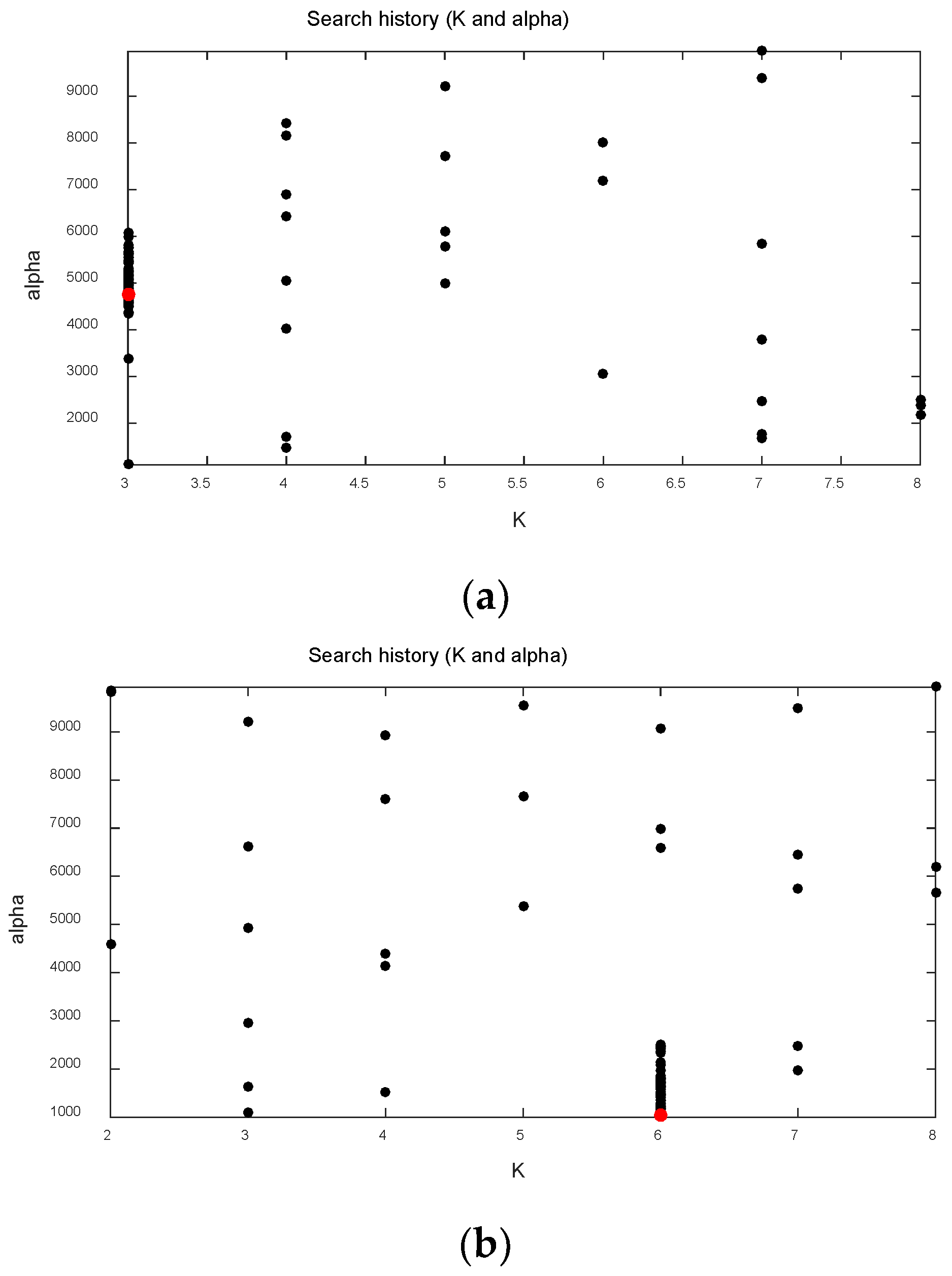
We used the above method, which is discussed in Section 3.2, to decompose the multi-GNSS sea level retrieval from the BRST station and HKQT station and selected the optimal combination of the decomposition mode number $K$ and penalty factor $\alpha$ of the VMD method. The parameters of the GOA were set as follows: search agent $n=25$ and maximum cycle number $L=15$. The best combination of parameters can be obtained through VMD decomposition and the GOA algorithm. As shown in Figure 4, historical search results were obtained using the GOA algorithm and objective function. For the BRST station, the optimal parameters of the VMD were $K=3$ and $\alpha$ =4800. For the HKQT station, the optimal parameters of the VMD were $K=6 \mathrm{and} \alpha =1000$. From Figure 5, it can be seen that after two iterations of the objective function, the optimal solution of the parameter tends to be stable, and the conclusion can be drawn that two iterations are needed to achieve the optimal result for the BRST and HKQT stations.

The iteration of objective function is as follows:

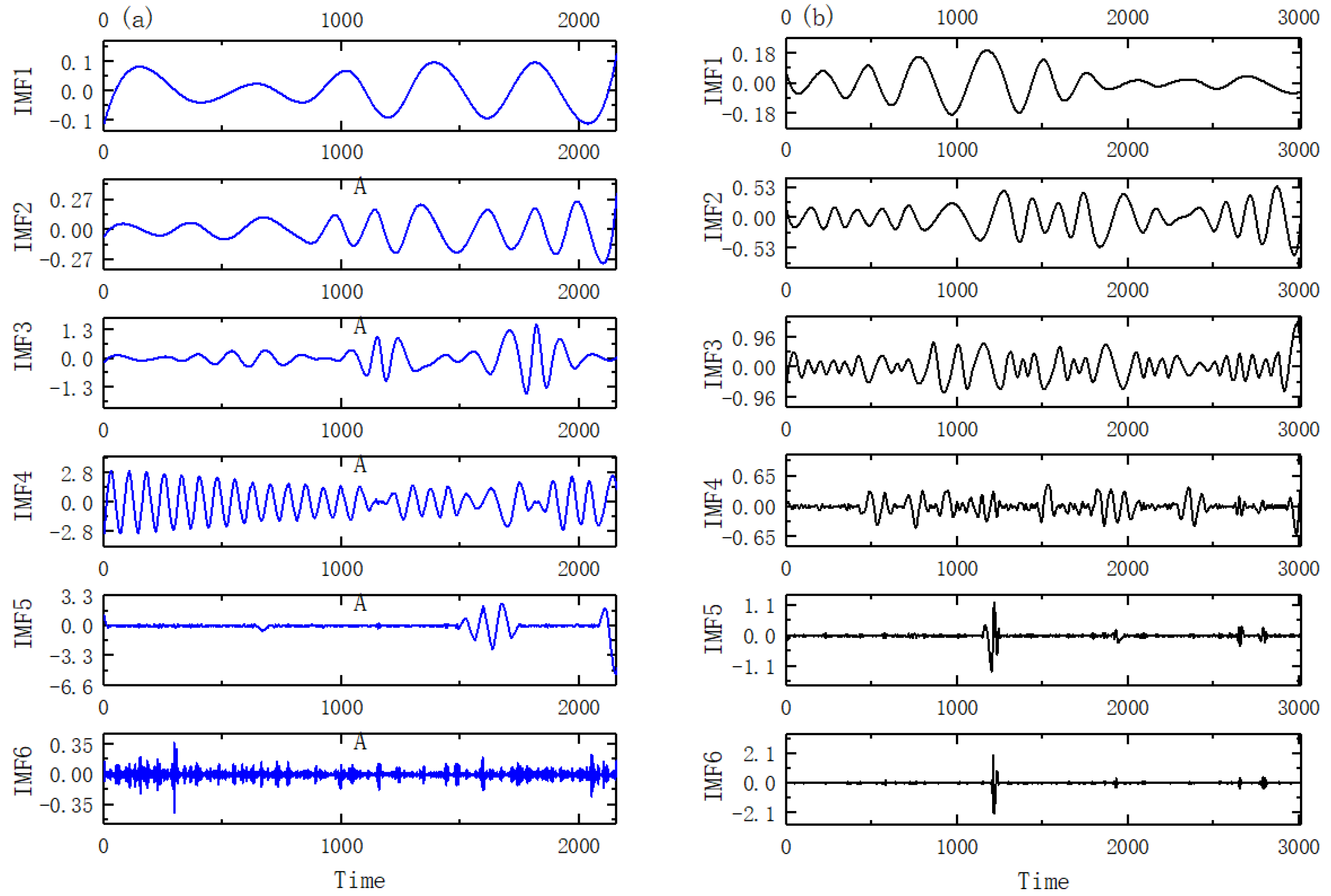
We used VMD to decompose the multi-GNSS sea level retrieval. Figure 6 shows the decomposition results. It can be seen from the figure that the IVMD decomposed the multi-GNSS sea level retrieval data from the BRST station and HKQT station into six IMFs. For the BRST station, the main information was extracted by the IMF1−IMF3 component; the IMF4−IMF6 may have contained noise mixed into the useful information. In order to distinguish useful information from the mixed-signal component, we used the composite evaluation index $T$, that is, to accumulate the modal component to reconstruct the time series, and calculated the composite evaluation index T value of the reconstructed time series. When $T$ reached a minimum, the rest of the IMF component was considered noise.

Table 1. Index T value of the different IMFs of BRST station retrieval.

Index	Reconstructed Time Series
	${\displaystyle {\displaystyle \sum }_{i=1}^1}\mathit{I}\mathit{M}{\mathit{F}}_{\mathit{i}}$	${\displaystyle {\displaystyle \sum }_{i=1}^2}\mathit{I}\mathit{M}{\mathit{F}}_{\mathit{i}}$	${\displaystyle {\displaystyle \sum }_{i=1}^3}\mathit{I}\mathit{M}{\mathit{F}}_{\mathit{i}}$
T	0.6659	0.3278	0.3341

shows the composite evaluation index $T$ for each reconstructed time series. As shown for the BRST station, when the time series reconstructed by the two modal components accumulated, the $T$ value reached its minimum. We can consider ${\sum }_{i=1}^{3}IM{F}_i$ as useful information that can be denoised. Similarly,

Table 2. Index T value of the different IMFs of T station retrieval.

Index	Reconstructed Time Series
	${\displaystyle {\displaystyle \sum }_{i=1}^1}\mathit{I}\mathit{M}{\mathit{F}}_{\mathit{i}}$	${\displaystyle {\displaystyle \sum }_{i=1}^2}\mathit{I}\mathit{M}{\mathit{F}}_{\mathit{i}}$	${\displaystyle {\displaystyle \sum }_{i=1}^3}\mathit{I}\mathit{M}{\mathit{F}}_{\mathit{i}}$	${\displaystyle {\displaystyle \sum }_{i=1}^4}\mathit{I}\mathit{M}{\mathit{F}}_{\mathit{i}}$	${\displaystyle {\displaystyle \sum }_{i=1}^5}\mathit{I}\mathit{M}{\mathit{F}}_{\mathit{i}}$	${\displaystyle {\displaystyle \sum }_{i=1}^6}\mathit{I}\mathit{M}{\mathit{F}}_{\mathit{i}}$
T	0.6145	0.1188	0.1159	0.1533	0.2467	0.3855

shows the composite evaluation index $T$ for each reconstructed time series for HKQT station. We can consider ${\sum }_{i=1}^{3}IM{F}_i$ as useful information that can be denoised for the HKQT station. Due to the different data time lengths and data differences between the two stations, the resulting VMD decompositions are also different.

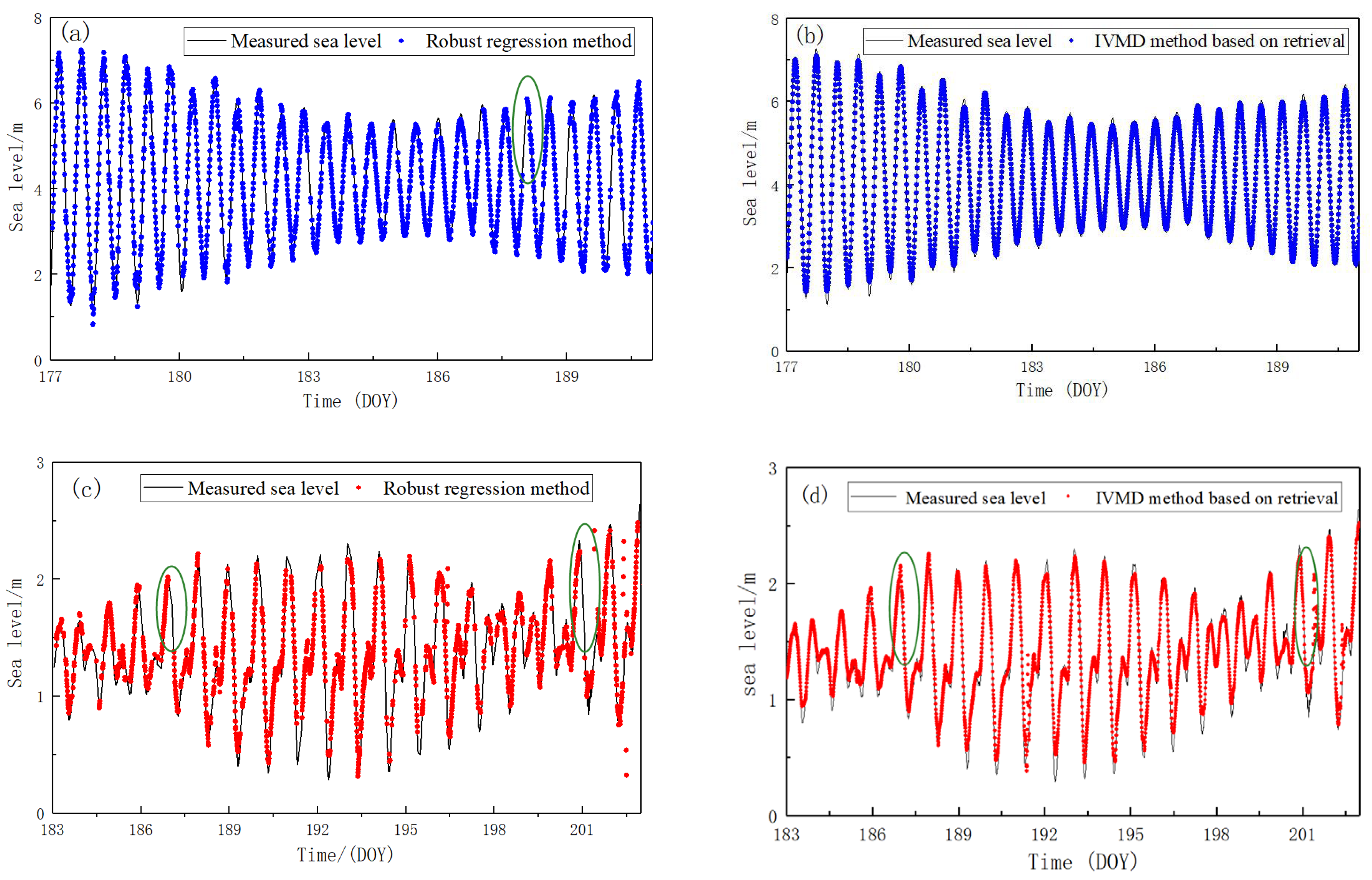
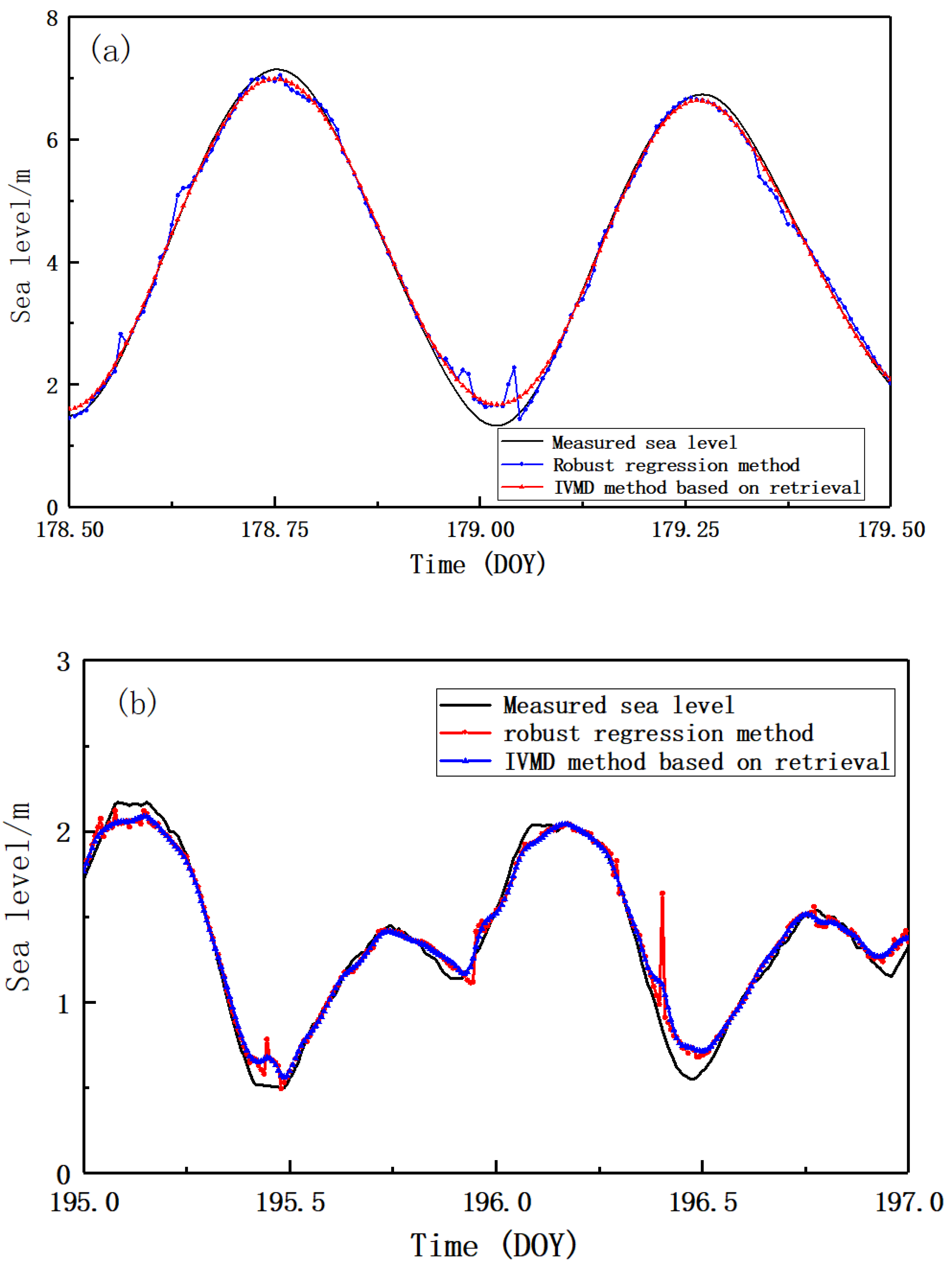
According to the above methods, after statistics, the results of the robust regression estimation and IVMD method for the BRST and HKQT stations are shown in

Table 3. RMSE and data loss rate of retrieval used in robust regression method and the IVMD algorithm for BRST and HKQT station.

Station Name	BRST		HKQT
Method	RMSE of retrieval (cm)	Loss rate of retrieval (%)	RMSE of retrieval (cm)	Loss rate of retrieval (%)
Robust regression method	10.78	8.01	10.86	33.25
IVMD method based on retrieval	8.78	0	9.78	0

. For BRST, the RMSE of the robust regression retrieval is 10.78 cm, and the data loss rate is 8.01%, where the loss rate represents the ratio of the number of windows without an output retrieval and the total number of windows. For HKQT, the RMSE of the robust regression was 10.86 cm, and the loss rate was 33.25%. The RMSE of the retrieval for the BRST station and HKQT station are 8.78 cm and 9.78 cm, respectively. As shown in Figure 7, the reason for the improved loss rate is clearly explained: the robust regression method caused some data to be missed in corresponding sliding time windows, resulting in data loss; however, there was no data loss from the IVMD algorithm because it used all multi-GNSS combination sea level retrieval data and could therefore supplement the lack of data in the multi-GNSS combination algorithm when the window retrieval data was insufficient. At the same time, through analyzing the retrieval used in the robust regression method and the IVMD algorithm for the BRST and HKQT stations during the DOY 178.5–179.5 and 195–197, respectively, as shown in Figure 8, the IVMD algorithm removed the influence of the low-quality signal outliers in the retrieval on the overall results. Comparing the IVMD method with the robust regression method, the accuracy of the BRST station improved by 24.3% and the accuracy of the HKQT station improved by 12.94%. In this study, we applied a 10 min combined time as the width of the windows for the sampling rate of the BRST and HKQT stations, and we can contain equal intervals of 10 min for multi-GNSS combination sea level retrieval to process the IVMD Algorithm, allowing us to receive 10 min equal interval sampling.

5. Conclusions

The combination method for multi-GNSS sea level retrieval based on sliding windows can effectively improve the accuracy and time resolution of sea level retrieval but cannot completely eliminate errors, and some low-quality signals in the window will affect the final accuracy of the overall retrieval. In addition, some windows lack data due to missing overflights in the corresponding timeframe, which may result in calculation and estimation failures in these windows. To solve this problem, this study proposes an IVMD method based on multi-GNSS combination sea level retrieval. We take energy entropy mutual information (EEMI) as an indicator and the sum of two EEMI modal functions as objective functions to develop the VMD algorithm.

Here, we targeted the problem that the traditional VMD method cannot determine the number of decomposed modal functions (IMF) and the value of penalty factors in the denoise process, which leads to an insufficient decomposition or an over-decomposition and causes the loss of part of the effective true information on the basis of the traditional VMD algorithm. Accordingly, the energy entropy mutual information was taken as the objective function, and the grasshopper optimization algorithm (GOA) was used to optimize the objective function. Thus, the number of modal decomposition and the value of the penalty factor are determined adaptively, and the denoise signal is determined by the composite index T.

The results of this study show that the sea level retrieval using a multi-GNSS combination based on the IVMD method can further improve the accuracy to <10 cm and can achieve 10 min equal interval sampling. Specifically, the robust regression method combines the retrieval of multiple constellations from multiple signals, whereas the IVMD method combines more input sea level retrievals from GNSS-MR. In other words, the robust regression method relies on internal retrieval consistency to avoid outliers, whereas the IVMD filtering method relies on external constraints and internal retrieval consistency to avoid overall accuracy reduction caused by outliers. In future, our research will try to apply IVMD filtering to LSP retrieval and skip robust regression, which will require allowing the existence of random noise in some prior RH.

References

1. Feng, G.; Jin, S.; Zhang, T. Coastal sea level changes in Europe from GPS, tide gauge, satellite altimetry and GRACE, 1993–2011. Adv. Space Res. 2013, 51, 1019–1028. [Google Scholar] [CrossRef]
2. Coleman, R. Satellite Altimetry and Earth Sciences: A Handbook of Techniques and Applications. Eos Trans. AGU 2001, 82, 376. [Google Scholar] [CrossRef]
3. Larson, K.M.; Löfgren, J.S.; Haas, R. Coastal sea level measurements using a single geodetic GPS receiver. Adv. Space Res. 2013, 51, 1301–1310. [Google Scholar] [CrossRef] [Green Version]
4. Small, E.E.; Larson, K.M.; Braun, J.J. Sensing vegetation growth with reflected GPS signals. Geophys. Res. Lett. 2010, 37, L12401. [Google Scholar] [CrossRef]
5. Larson, K.M.; Small, E.E.; Gutmann, E.; Bilich, A.; Axelrad, P.; Braun, J. Using GPS multipath to measure soil moisture fluctuations: Initial results. GPS Solut. 2008, 12, 173–177. [Google Scholar] [CrossRef]
6. Larson, K.M.; Gutmann, E.D.; Zavorotny, Z.U.; Braun, J.J.; Williams, M.W.; Nievinski, F.G. Can we measure snow depth with GPS receivers? Geophys. Res. Lett. 2009, 36, L17502. [Google Scholar] [CrossRef] [Green Version]
7. Schöne, T.; Schön, N.; Thaller, D. IGS tide gauge benchmark monitoring pilot project (TIGA): Scientific benefits. J. Geod. 2009, 83, 249–261. [Google Scholar] [CrossRef]
8. Hall, C.; Cordey, R. Multistatic scatterometry. In Proceedings of the International Geoscience and Remote Sensing Symposium, ‘Remote Sensing: Moving toward the 21st Century’, Edinburgh, UK, 12–16 September 1988. [Google Scholar] [CrossRef]
9. Nakashima, Y.; Heki, K. GPS Tide Gauges Using Multipath Signatures. J. Geod. Soc. Jpn. 2013, 59, 157–162. [Google Scholar]
10. Löfgren, J.S.; Haas, R. Sea level measurements using multi-frequency GPS and GLONASS observations. EURASIP J. Adv. Signal Process. 2014, 2014, 50. [Google Scholar] [CrossRef] [Green Version]
11. Jin, S.; Zhang, Q.; Qian, X. New Progress and Application Prospects of Global Navigation Satellite System Reflectometry (GNSS + R). Acta Geod. Cartogr. Sin. 2017, 46, 1389–1398. [Google Scholar]
12. Ansari, K.; Seok, H.W.; Jamjareegulgarn, P. Quasi zenith satellite system-reflectometry for sea-level measurement and implication of machine learning methodology. Sci. Rep. 2022, 12, 21445. [Google Scholar] [CrossRef]
13. Löfgren, J.S.; Haas, R.; Scherneck, H.G. Sea level time series and ocean tide analysis from multipath signals at five GPS sites in different parts of the world. J. Geodyn. 2014, 80, 66–80. [Google Scholar] [CrossRef] [Green Version]
14. Tabibi, S.; Geremia-Nievinski, F.; Francis, O.; Dam, T.V. Tidal analysis of gnss reflectometry applied for coastal sea level sensing in antarctica and greenland. Remote Sens. Environ. 2020, 248, 111959. [Google Scholar] [CrossRef]
15. Williams, S.D.P.; Nievinski, F.G. Tropospheric delays in ground-based GNSS multipath reflectometry—Experimental evidence from coastal sites. J. Geophys. Res. Solid Earth 2017, 122, 2310–2327. [Google Scholar] [CrossRef] [Green Version]
16. Purnell, D.J.; Gomez, N.; Chan, N.H.; Strandberg, J.; Holland, D.M.; Hobiger, T. Quantifying the Uncertainty in Ground-Based GNSS-Reflectometry Sea Level Measurements. IEEE J. Sel. Top. Appl. Earth Obs. Remote Sens. 2020, 13, 4419–4428. [Google Scholar] [CrossRef]
17. Strandberg, J.; Hobiger, T.; Haas, R. Improving GNSS-R sea level determination through inverse modeling of SNR data. Radio Sci. 2016, 51, 1286–1296. [Google Scholar] [CrossRef] [Green Version]
18. Santamaría-Gómez, A.; Watson, C.; Gravelle, M.; King, M.; Wöppelmann, G. Levelling co-located GNSS and tide gauge stations using GNSS reflectometry. J. Geod. 2015, 89, 241–258. [Google Scholar] [CrossRef]
19. Santamaría-Gómez, A.; Watson, C. Remote leveling of tide gauges using GNSS reflectometry: Case study at Spring Bay, Australia. GPS Solut. 2016, 21, 451–459. [Google Scholar] [CrossRef]
20. Wang, X.; Zhang, Q.; Zhang, S. Water levels measured with SNR using wavelet decomposition and Lomb–Scargle periodogram. GPS Solut. 2018, 22, 22. [Google Scholar] [CrossRef]
21. Wang, X.; He, X.; Zhang, Q. Coherent superposition of multi-GNSS wavelet analysis periodogram for sea-level retrieval in GNSS multipath reflectometry. Adv. Space Res. 2019, 65, 1781–1788. [Google Scholar] [CrossRef]
22. Zhang, S.; Liu, K.; Liu, Q.; Zhang, C.; Zhang, Q.; Nan, Y. Tide Variation Monitoring Based Improved GNSS-MR by Empirical Mode Decomposition. Adv. Space Res. 2019, 63, 3333–3345. [Google Scholar] [CrossRef]
23. Strandberg, J.; Hobiger, T.; Haas, R. Real-time sea-level monitoring using Kalman filtering of GNSS-R data. GPS Solut. 2019, 23, 61. [Google Scholar] [CrossRef] [Green Version]
24. Roussel, N.; Ramillien, G.; Frappart, F.; Darrozes, J.; Gay, A.; Biancale, R.; Striebig, N.; Hanquiez, V.; Bertin, X.; Allain, D. Sea level monitoring and sea state estimate using a single geodetic receiver. Remote Sens. Environ. 2015, 171, 261–277. [Google Scholar] [CrossRef]
25. Wang, X.; He, X.; Zhang, Q. Evaluation and combination of quad-constellation multi-GNSS multipath reflectometry applied to sea level retrieval. Remote Sens. Environ. 2019, 231, 111229. [Google Scholar] [CrossRef]
26. Tabibi, S.; Geremia-Nievinski, F.; Dam, T.V. Statistical comparison and combination of GPS, GLONASS, and multi-GNSS multipath reflectometry applied to snow depth retrieval. IEEE Trans. Geosci. Remote Sens. 2017, 55, 3773–3785. [Google Scholar] [CrossRef]
27. Reinking, J. GNSS-SNR water level estimation using global optimization based on interval analysis. J. Geod. Sci. 2016, 6, 80–92. [Google Scholar] [CrossRef]
28. Dragomiretskiy, K.; Zosso, D. Variational Mode Decomposition. IEEE Trans. Signal Process 2014, 62, 531–544. [Google Scholar] [CrossRef]
29. Shen, Y.; Zheng, W.; Yin, W.; Xu, A.; Zhu, H. Feature Extraction Algorithm Using a Correlation Coefficient Combined with the VMD and Its Application to the GPS and GRACE. IEEE Access 2021, 9, 17507–17519. [Google Scholar] [CrossRef]
30. Zhang, X.; Miao, Q.; Zhang, H.; Wang, L. A parameter-adaptive VMD method based on grasshopper optimization algorithm to analyze vibration signals from rotating machinery. Mech. Syst. Signal Process 2018, 108, 58–72. [Google Scholar] [CrossRef]
31. Ahmed, W.A.; Wu, F.; Marlia, D.; Zhao, Y. Mitigation of Ionospheric Scintillation Effects on GNSS Signals with VMD-MFDFA. Remote Sens. 2019, 11, 2867. [Google Scholar] [CrossRef] [Green Version]
32. Zhou, C.; Ma, J.; Wu, J.; Yuan, X. An adaptive VMD method based on improved GOA to extract early fault feature of rolling bearings. Int. J. Innov. Comput. Inf. Control. 2019, 15, 1485–1505. [Google Scholar]
33. Li, C.; Liu, Y.; Liao, Y. An Improved Parameter-Adaptive Variational Mode Decomposition Method and Its Application in Fault Diagnosis of Rolling Bearings. Shock Vib. 2021, 2021, 2968488. [Google Scholar] [CrossRef]
34. Yang, Y.; Song, L.; Xu, T. Robust estimator for correlated observations based on bifactor equivalent weights. J. Geod. 2002, 76, 353–358. [Google Scholar] [CrossRef]
35. Dabbakuti, J.R.K.K.; Jacob, A.; Veeravalli, V.R.; Kallakunta, R.K. Implementation of IoT analytics ionospheric forecasting system based on machine learning and ThingSpeak. IET Radar Sonar Navig. 2020, 14, 341–347. [Google Scholar] [CrossRef]
36. Saremi, S.; Mirjalili, S.; Lewis, A. Grasshopper optimisation algorithm: Theory and application. Adv. Eng. Softw. 2017, 105, 30–47. [Google Scholar] [CrossRef] [Green Version]
37. He, X.; Bos, M.S.; Montillet, J.P.; Fernandes, R.; Melbourne, T.; Jiang, W.; Li, W. Spatial Variations of Stochastic Noise Properties in GPS Time Series. Remote Sens. 2021, 13, 4534. [Google Scholar] [CrossRef]
38. Silva, L.K.J.; Ramarakula, M. An efficient interference mitigation approach for NavIC receivers using improved variational mode decomposition and wavelet packet decomposition. Trans. Emerg. Telecommun. Technol. 2021, 32, e4242. [Google Scholar]
39. Zhu, J.; Zhang, Z.; Kuang, C. A Reliable Evaluation Indicator of Wavelet Denoising. Geomat. Inf. Sci. Wuhan Univ. 2015, 40, 688–694. [Google Scholar]
Figure 1. Number of available SNR arcs per day: (a) for the BRST station, the number of available SNR arcs from quad-constellation per day during DOY 177–191 2021; (b) for the HKQT station, the number of available SNR arcs from quad-constellation per day during DOY 183–203 2021.
Remotesensing 15 01733 g001
Figure 2. Number of RH points in each window: (a) for the BRST station, the number of RH points in each window during DOY 177–191, 2021; (b) for the HKQT station, the number of RH points in each window during DOY 177–191, 2021.
Remotesensing 15 01733 g002
Figure 3. IVMD method flowchart based on multi-GNSS combination sea level retrieval.
Remotesensing 15 01733 g003
Figure 4. Search history (K and alpha): (a) Historical value for the BRST station; (b) historical value for the HKQT station.
Remotesensing 15 01733 g004
Figure 5. Convergence of the objective function of the station retrieval data: (a) for the BRST station, the convergence of the objective function; (b) for the HKQT station, the convergence of the objective function.
Remotesensing 15 01733 g005
Figure 6. VMD decomposition based on the station retrieval data: (a) for the BRST station; (b) for the HKQT station.
Remotesensing 15 01733 g006
Figure 7. Results of robust regression and IVMD algorithm for the stations: (a) the results of robust regression algorithm for the BRST during DOY 177–191, 2021; (b) results of IVMD algorithm for the BRST during DOY 177–191; (c) results of robust regression algorithm for the HKQT during DOY 177–191; (d) results of IVMD algorithm for the HKQT during DOY 177–191.
Remotesensing 15 01733 g007
Figure 8. Comparison of the result of stations retrieval: (a) comparison between the results of robust regression and IVMD algorithm for the BRST station during DOY 177–191, 2021; (b) comparison between the results of robust regression and IVMD algorithm for the HKQT station during DOY 177–191, 2021.
Remotesensing 15 01733 g008