Prediction of the Area of High-Turbidity Water in the Yatsushiro Sea, Japan, Using Machine Learning with Satellite, Meteorological, and Oceanographic Data

Abstract

Turbid water is known to affect aquatic ecosystems. If the spread of turbid water can be predicted, it is expected to lead to the prediction of damage caused by turbid water in rich aquatic ecosystems and aquaculture farms, and to countermeasures against turbid water. In this study, we developed a method for predicting the area of high-turbidity water using machine learning with satellite-observed total suspended solids (TSS) product and relatively readily available meteorological and oceanographic data (rainfall, wind direction and speed, atmospheric pressure, and tide level) in the past and evaluated it for the Kuma River estuary of the Yatsushiro Sea in Japan. The results showed that the highest accuracy was obtained using random forest regression, with a coefficient of determination of 0.552, when the area of high-turbidity water based on the previous day’s TSS product and hourly meteorological and oceanographic data from the previous day were used as inputs. The most important factor for the prediction was the area of high-turbidity water, followed by wind, and tide level, but the effect of rainfall was small, which was probably due to the flood-control function of the river. Our future work will be to evaluate the applicability of the method to other areas, improve the accuracy, and predict the distribution area.

1. Introduction

The preservation of the aquatic environment is an important issue for modern society. Turbid water is known to affect organisms living in the aquatic environment, and an accurate understanding of turbid water is useful in confirming the state of pollution. There are various substances that cause turbid water, ranging from inorganic substances such as sand and gravel to organic substances such as leaves and plankton. In particular, insoluble inorganic and organic matter that is less than 2 mm and greater than 1 μm is called total suspended solids (TSS) [1].

Many researchers have studied the effects of turbid water on aquatic ecosystems. For example, it has been confirmed that although “sand discharge”, which is the discharge of sand and other substances that accumulate in dams downstream, is not directly related to fish injury or mortality, it causes stress to fish by raising their hemoglobin levels when concentrations are high [2,3,4,5]. Cases of fish showing avoidance behavior toward turbid water have also been reported [4]. In addition, when the particle size of suspended solids in turbid water exceeds a range of 1.237–35.977 μm, they tend to adhere to the gills, leading to gill blockage [6]. As for tuna, it is said that tuna are susceptible to the effects of harmful algae such as red tide because they require a large amount of oxygen and take in large amounts of seawater at a time [7]. In the case of a large number of bluefin tuna dying due to a red tide in a tuna aquaculture fishery, it was pointed out that the high concentration of turbid water made the tuna less visible in the water, causing them to come into contact with nets and other objects, resulting in injuries [8]. In addition to fish, turbid water also adversely affects the growth of brown algae such as wakame and kajime seaweed. For example, it has been reported that suspended solids inhibit the sedimentation of migratory spores produced by brown algae, increasing the time required for their attachment, which leads to a decrease in brown algae [9]; it has also been reported that suspended solids inhibit the attachment of Nori shell spores [10,11].

If the turbid water spreads to areas with rich aquatic ecosystems and aquaculture farms, the damage described above is expected to become more pronounced. However, if its characteristics and scale can be predicted in advance, it could be used to predict damage and evacuate aquaculture facilities. There are several examples of studies on the prediction of turbidity: Wang et al. (2021) focused on the relationship between turbidity and tidal level and compared and evaluated several methods for predicting turbidity areas based on tidal level [12]. The results showed that an artificial neural network method that uses the tide level as an input and the turbidity index “Nephelometric Turbidity Unit (NTU)” obtained from buoys installed in coastal areas as an output has the highest accuracy, and that the two previous tidal cycles, excluding the forecast period, are important for the input tide-level data. The input tide-level data are important for the previous two tidal cycles, excluding the time of the forecast. Turbidity prediction based on weather information was studied by Zhang et al. (2021) and Tsai et al. (2017) [13,14]. Zhang et al. developed a method to predict lake turbidity information obtained from smartphone photography by inputting wind speed, wind direction, temperature, and rainfall into a random forest [13]. The coefficient of determination is more than 0.89, and the most important input parameters are wind direction and wind speed. Tsai et al. developed a model to predict weir turbidity from rainfall and water volume and obtained 5.787 as the mean-square error [14]. Alizadeh et al. (2018) used buoys placed at an estuary to obtained data on turbidity, water temperature, salinity, etc., and river flow data were used to study a method for predicting turbidity in estuaries [15]. The results showed that the river flow of one hour before was important for the prediction; Kumar et al. (2022) predicted turbidity at multiple sites in an estuary in Hong Kong based on meteorological information, pH, and oxygen-dissolved solids [16]. As a result, they achieved an average prediction accuracy of 88.45% with LSTM-RNN. However, since most existing studies focus on turbidity, it is difficult to capture the area of turbid water. In addition, they often use detailed field data, which are difficult to apply in places where the observation environment is not well-developed.

Based on this background, we propose a machine learning method to predict the area of high-turbidity water around an estuary on the following day, using satellite TSS products and easily obtainable local meteorological and oceanographic data as inputs, using the Yatsushiro Sea in Japan as the study area. We believe that the prediction of the area of high-turbidity water using these types of data is a unique attempt not seen in previous studies. For machine learning, Support Vector Regression (SVR) and Random Forest Regression (RFR) are evaluated in terms of accuracy. Satellite data will be used for the TSS product using Geostationary Ocean Color Imager-I (GOCI-I) [17,18], which is capable of observing coastal areas at high frequency from geostationary orbit.

2. Materials and Methods

2.1. Satellite-Based TSS Observations and GOCI

Sensors such as GOCI, the Second-generation Global Imager (SGLI) onboard Global Change Observation-Climate (GCOM-C), and the Moderate Resolution Imaging Spectroradiometer (MODIS) instruments onboard the Terra and Aqua satellites have bands suitable for observing coastal areas and are capable of estimating TSS [19,20]. In this type of sensor, although GOCI has a lower spatial resolution (500 m) than SGLI and MODIS and its observation area is limited to East Asia, it is capable of TSS observation with high frequency (eight times a day) from a geostationary orbit and cloud removal by time-series composite [17]. Since no other satellite sensor has these characteristics, we selected the TSS product of the GOCI-I instrument for this study, although it is limited to analysis of sea areas that do not include narrow bays.

Table 1. Spectral bands of the GOCI-I instrument.

Band	Center Wavelength	Band Width	Spatial Resolution
1	412 nm	20 nm	500 m
2	443 nm	20 nm
3	490 nm	20 nm
4	555 nm	20 nm
5	660 nm	20 nm
6	680 nm	10 nm
7	745 nm	20 nm
8	865 nm	40 nm

shows the spectral bands of the GOCI-I instrument [21]. The TSS product of GOCI-I is calculated from the visible bands at 490 nm and 745 nm by the following equation [22].

$$\mathrm{TSS}={10}^{1.0758+1.1230\times Rrs\left(745\right)/Rrs\left(490\right)},$$

(1)

where R_rs(490) and R_rs(745) are the remote sensing reflectance values for the 490 nm and 745 nm bands, respectively. This equation is less accurate when TSS is low in concentration and should be used with caution in the open ocean but provides more reliable TSS information in coastal areas where TSS is generally high in concentration [22].

2.2. Proposed Method

In this study, we propose a method to predict the area of high-turbidity water one day later by machine learning using satellite-based TSS products and local meteorological and oceanographic data, acquired over the past several days. Local meteorological and oceanographic data should be parameters that are closely related to turbidity; in this study, wind direction and speed, and tide level, were selected based on the work of Zhang et al. [13] and Wang et al. [12], and rainfall and pressure were selected based on the work of Kumar et al. [16]. It is known that glacial meltwater can affect turbidity in the presence of glacial meltwater [23], but this effect was not considered in this study area, which is located at mid-latitudes.

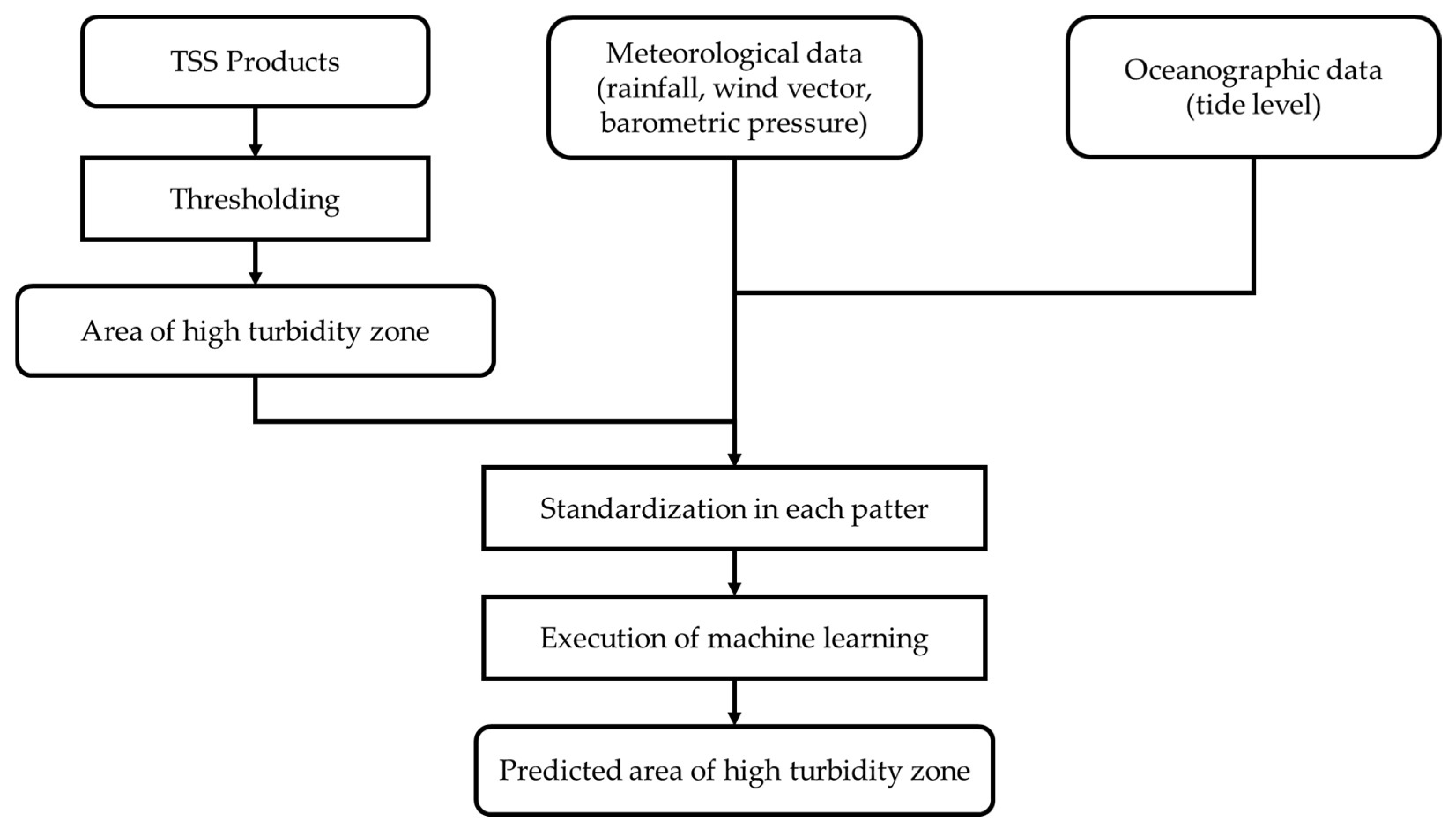
The processing procedure of the proposed method is as follows.

• In the target area, using a specific time T of the prediction day as the prediction reference, collect a satellite-based TSS product at time T one day ago, and rainfall, wind speed and direction, pressure, and tide-level data for each hour from 1 to N days ago. That is, the input TSS image is one image, whereas the meteorological and oceanographic data are 24 data per day (from time T to 23 h before that time).
• Binarize the TSS product by thresholding based on the presence or absence of high-turbidity water. The number of high-turbid water pixels in the binarized TSS image is then counted to obtain the area of high-turbidity zone.
• Standardize the area of the high-turbidity water based on satellite observations, and the four meteorological and oceanographic parameters to have a mean of 0 and a standard deviation of 1, respectively, and apply these values to the learned machine learning model to regressively estimate the area of high-turbidity water (normalized value) for the prediction day. The machine learning model needs to be trained in advance using training data sets for each of the prediction dates for which TSS data were available.

Figure 1 shows the above process flow. In the proposed method, the importance of each input data and the value of N are evaluated in the sections that follow. We also compare and evaluate SVR and RFR as the machine learning model.

2.3. Study Area

In this study, a part of the Yatsushiro Sea, Japan, defined as the region of (32.43°N, 130.58°E) to (32.54°N, 130.42°E) including the estuary of the Kuma River (around 32.50°N, 130.57°E) flowing through Kumamoto Prefecture, was selected as the study area. The location of the study area is shown in Figure 2. The Yatsushiro Sea is relatively calm because it is an inland sea surrounded by the Kyushu mainland and the Amakusa Islands. This sea is rich in fishery resources, especially in the cultivation of sea bream, yellowtail, nori, tiger prawn, and pearls [24]. We chose this area rather than a larger area because the range of turbidity variation and the mechanism of turbidity are different in the coastal and open ocean areas, and the coastal areas generally have diverse aquatic ecosystems and are important for aquaculture.

2.4. Data Used

The period covered by this study was defined as 11 years, from 2011 to 2021.

TSS products were obtained from data observed by GOCI-I at 10:16 UTC (1:16 UTC) during this period, and only those data with cloud coverage of 10% or less in the target water area were selected. In addition, a cutout was made from each TSS image to include the study area according to the turbid water coverage of each image, and only pure water pixels without land were selected using a land mask created from coastline vector data and high-resolution satellite imagery. Then, of all the TSS data obtained, one set of TSS images was defined as those obtained for two consecutive days. As a result, a total of 219 TSS data sets were obtained for the study period under study.

Next, for each of the 219 datasets, hourly meteorological and oceanographic data were obtained from the Japan Meteorological Agency (JMA) website for each day up to nine days prior to the prediction date [26]. Rainfall data were obtained from the Automated Meteorological Data Acquisition System (AMeDAS) [27] at eight sites located in the catchment area of the Kuma River (Yatsushiro, Isshochi, Yamae, Hitoyoshi, Itsuki, Kami, Taraki, and Yamae-Yokoya). Wind direction and speed data were obtained from AMeDAS at one location (Yatsushiro) near the mouth of the river, and east–west and north–south vectors were calculated from these data and used as input data (for example, for a 2 m wind speed from the east-southeast, the east–west vector is 1.848 m/s and the north–south vector is −0.766 m/s). The barometric pressure was obtained from the nearest meteorological observatory (Hitoyoshi) from the mouth of the river. Figure 3 shows the location of each observation station.

For tide data, we used astronomical tide data near the mouth of the river (Yatsushiro) provided by JMA [28]. Astronomical tide level is a predicted value of the change in tide level caused by lunar and solar tidal forces, and although it differs from the actual measured tide level, it was adopted because it is readily available.

In applying the above data to machine learning, the 219 data sets were divided in half, with 109 sets for training and 110 sets for testing.

2.5. Evaluation Method

2.5.1. Evaluation (A)

In Section 2.2, Procedure (1), N is the number of days back for the meteorological/oceanographic data to be input. In this study, nine cases were evaluated, ranging from N = 9 (using data from one to nine days before the prediction date) to N = 1 (using only data from one day before). In addition, for SVR, the radial basis function (RBF) was applied with epsilon = 0.1 and 0.01, and the cost parameter C = 1 and 10 for SVR; and the number of trees, trees = 100 and 1000, and the maximum depth of each tree, depth = 100 and 1000, were investigated for RFR. Thus, combining these conditions, the total number of cases evaluated is 9 (N) × { 4 (SVR parameters) + 4 (RFR parameters) } = 72 cases.

2.5.2. Evaluation (B)

In Evaluation (A), N means that all meteorological and oceanographic data for each day from 1 to N days before the prediction date are used, but alternatively, a model that uses only meteorological and oceanographic data from n days ago is also possible. Therefore, we evaluated this alternate model by inputting only the meteorological and oceanographic data from n days ago and no TSS images to each machine learning model. In this case, the number of evaluation cases is 9 (n) × { 4 + 4 } = 72 cases.

2.5.3. Evaluation (C)

Using the model that showed the highest accuracy in evaluations (A) and (B), we evaluated the impact of each input parameter on estimation accuracy by training the model using only one of the five input parameters: TSS, rainfall, wind direction and speed, barometric pressure, and tide level.

3. Results

3.1. TSS Image and Its Binarization

Figure 4 shows the Landsat 8 image at 9:45 on 17 November 2020 JST and the TSS image of GOCI-I and its binarized image at 10:16 on the same day as an example. In the binarized TSS image (c), pixels with high turbidity were selected from the original TSS image (b) with a threshold of 4 mg/L. The area of high-turbidity water in this example is 20.50 km² (=82 pixels), and its normalized area is 0.390, where each normalized area was obtained by dividing each area of high-turbidity water by the maximum area of high-turbidity water of 52.50 km² (=210 pixels) obtained from all data from 2011 to 2021.

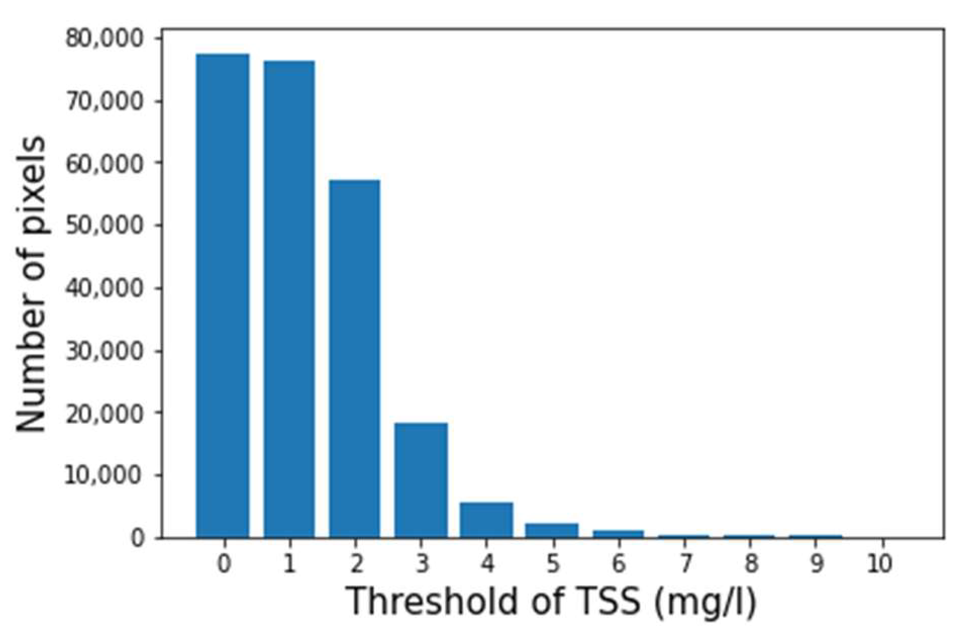
Figure 5 shows the relationship between the threshold value for extracting high-turbidity water and the number of pixels extracted as high-turbidity pixels. In the case of the threshold value of 4 mg/L used in this study, the number of extracted high-turbidity pixels corresponds to approximately 10% of the total number of water pixels.

3.2. Results of Evaluation (A)

Table 2. Coefficient of determination (R²), correlation coefficient (R), and RMSE (km²) for each model in each case of N = 1 to 9 in Evaluation (A).

Model	Index	N = 1	N = 2	N = 3	N = 4	N = 5	N = 6	N = 7	N = 8	N = 9
SVR (ε = 0.1, C = 1.0)	R2	0.237	0.109	0.073	0.050	0.021	0.028	0.018	−0.016	−0.034
	R	0.561	0.433	0.390	0.381	0.343	0.350	0.326	0.271	0.238
	RMSE (km2)	9.463	10.234	10.435	10.569	10.725	10.684	10.742	10.928	11.026
SVR (ε = 0.01, C = 1.0)	R2	0.373	0.222	0.140	0.132	0.107	0.108	0.096	0.068	0.046
	R	0.635	0.506	0.388	0.381	0.345	0.348	0.329	0.270	0.228
	RMSE (km2)	8.579	9.559	10.054	10.096	10.241	10.232	10.308	10.467	10.587
SVR (ε = 0.1, C = 10.0)	R2	0.251	0.120	0.097	0.066	0.017	0.056	0.025	−0.013	−0.030
	R	0.568	0.429	0.417	0.388	0.337	0.350	0.329	0.284	0.257
	RMSE (km2)	9.375	10.165	10.287	10.465	10.727	10.527	10.706	10.907	11.005
SVR (ε = 0.01, C = 10.0)	R2	0.402	0.248	0.194	0.161	0.111	0.137	0.107	0.072	0.056
	R	0.645	0.511	0.459	0.422	0.371	0.378	0.340	0.283	0.255
	RMSE (km2)	8.378	9.389	9.718	9.910	10.198	10.059	10.242	10.438	10.534
RFR (trees = 100, depth = 100)	R2	0.552	0.532	0.544	0.531	0.519	0.480	0.518	0.504	0.493
	R	0.746	0.743	0.742	0.741	0.729	0.710	0.738	0.718	0.719
	RMSE (km2)	7.260	7.418	7.326	7.425	7.521	7.821	7.531	7.640	7.723
RFR (trees = 1000, depth = 100)	R2	0.530	0.524	0.524	0.509	0.511	0.517	0.520	0.515	0.516
	R	0.737	0.736	0.736	0.726	0.725	0.728	0.729	0.725	0.725
	RMSE (km2)	7.436	7.478	7.483	7.596	7.581	7.535	7.514	7.552	7.547
RFR (trees = 100, depth = 1000)	R2	0.537	0.517	0.526	0.520	0.472	0.525	0.534	0.512	0.520
	R	0.744	0.729	0.738	0.730	0.709	0.735	0.736	0.724	0.729
	RMSE (km2)	7.380	7.537	7.462	7.514	7.880	7.476	7.404	7.577	7.516
RFR (trees = 1000, depth = 1000)	R2	0.538	0.520	0.520	0.517	0.511	0.509	0.515	0.508	0.515
	R	0.741	0.734	0.731	0.729	0.726	0.725	0.726	0.721	0.725
	RMSE (km2)	7.370	7.516	7.513	7.539	7.586	7.599	7.553	7.605	7.549

shows the root mean-square error (RMSE) of the coefficient of determination (R²), correlation coefficient (R), and area (km²) for each result. The results show that SVR has a low R² and is unreliable, while RFR has a high R² and has the potential to make predictions. The most accurate model was RFR with N = 1 and trees = 100 and depth = 100, resulting in R² = 0.552, R = 0.746, and RMSE = 7.260 km² (0 to a maximum of 52.50 km²). In addition,

Table 3. Feature importance analysis results for N = 1 to 9 for each input variable in RFR: rainfall (RF), wind vector (WV), barometric pressure (BP), tide level (TL), and area of high-turbidity water (HT).

Model	Variable	N = 1	N = 2	N = 3	N = 4	N = 5	N = 6	N = 7	N = 8	N = 9
RFR (trees = 100, depth = 100)	RF	0.001	0.012	0.033	0.039	0.051	0.058	0.068	0.053	0.032
	WV	0.238	0.252	0.242	0.238	0.204	0.202	0.223	0.234	0.224
	BP	0.012	0.015	0.018	0.012	0.015	0.021	0.016	0.020	0.021
	TL	0.062	0.085	0.070	0.085	0.109	0.111	0.084	0.115	0.097
	HT	0.688	0.637	0.637	0.626	0.621	0.608	0.609	0.578	0.626
RFR (trees = 1000, depth = 100)	RF	0.001	0.017	0.032	0.047	0.045	0.048	0.048	0.046	0.044
	WV	0.249	0.242	0.233	0.217	0.224	0.223	0.229	0.230	0.236
	BP	0.013	0.014	0.017	0.016	0.016	0.017	0.016	0.018	0.017
	TL	0.075	0.077	0.085	0.096	0.100	0.095	0.098	0.105	0.106
	HT	0.662	0.650	0.633	0.624	0.615	0.617	0.608	0.601	0.597
RFR (trees = 100, depth = 1000)	RF	0.001	0.023	0.030	0.040	0.059	0.034	0.048	0.044	0.031
	WV	0.263	0.229	0.229	0.229	0.219	0.232	0.235	0.242	0.231
	BP	0.015	0.017	0.022	0.015	0.014	0.021	0.015	0.020	0.022
	TL	0.075	0.100	0.079	0.082	0.094	0.079	0.081	0.077	0.106
	HT	0.646	0.631	0.641	0.635	0.614	0.634	0.621	0.617	0.609
RFR (trees = 1000, depth = 1000)	RF	0.001	0.017	0.033	0.048	0.042	0.044	0.055	0.046	0.049
	WV	0.250	0.248	0.229	0.219	0.223	0.221	0.226	0.233	0.229
	BP	0.013	0.014	0.016	0.015	0.015	0.017	0.018	0.017	0.016
	TL	0.068	0.078	0.088	0.091	0.096	0.101	0.092	0.110	0.102
	HT	0.668	0.643	0.634	0.626	0.625	0.616	0.609	0.594	0.603

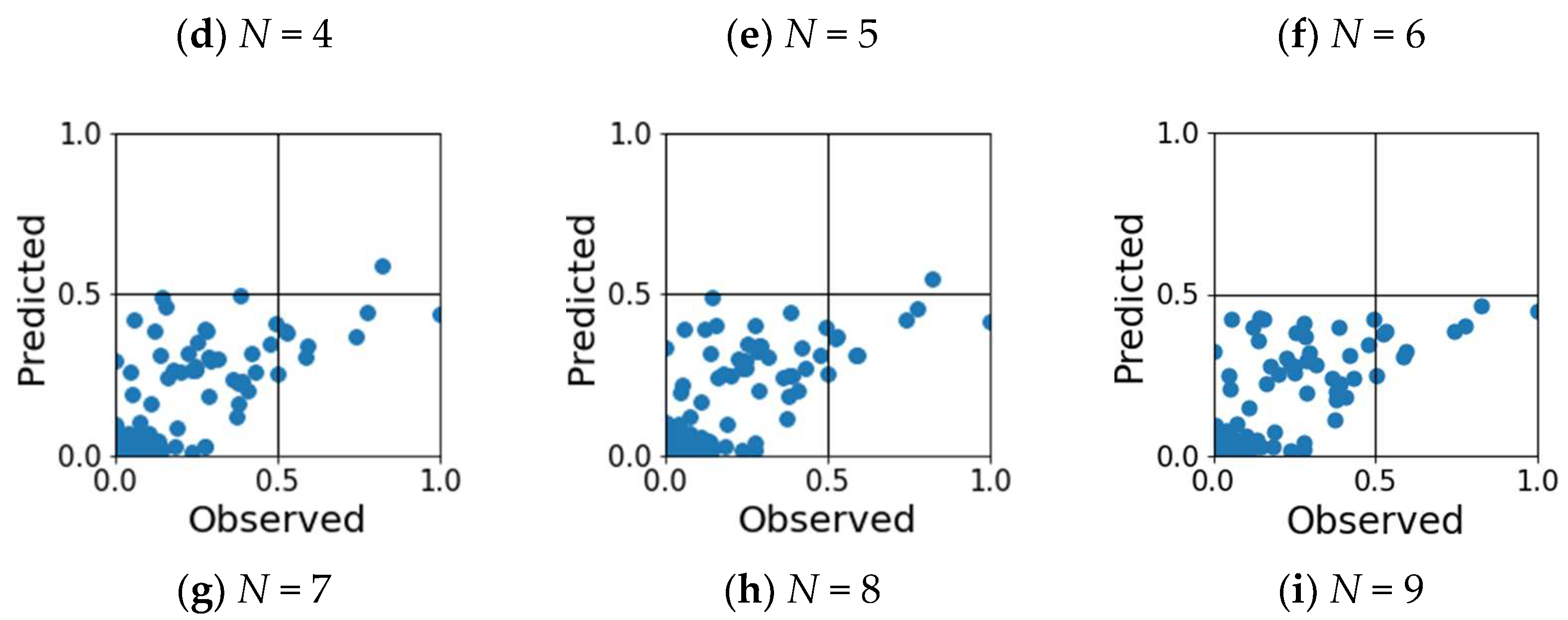
shows the results of feature importance (FE) analysis for each input variable: rainfall (RF), wind vector (WV), barometric pressure (BP), tide level (TL), and area of high-turbidity water (HT). From this table, it can be seen that the factor that most influences the prediction is the area of high-turbidity water on the previous day, followed by wind and tide level. Figure 6 is a scatterplot showing the relationship between the observed and predicted normalized high-turbidity area for each case of N = 1 to 9 in evaluation (A) using RFR with trees = 100 and depth = 100.

Figure 6 shows several outliers. Investigation of these outliers revealed that some of them are often caused by several consecutive days of strong winds. Therefore, from the 219 training data, we excluded the five data sets that had five consecutive days with daily maximum values of instantaneous wind speeds exceeding 10 m, and trained the RFR (trees = 100, depth = 100). The obtained coefficients of determination, correlation coefficients, and RMSE are shown in

Table 4. Coefficient of determination (R²), correlation coefficient (R), and RMSE (km²) in each case of N = 1 to 9 using the best model (RFR with trees = 100 and depth = 100) trained by the data excluding samples of five or more consecutive days with maximum instantaneous wind speeds exceeding 10 m.

Model	Index	N = 1	N = 2	N = 3	N = 4	N = 5	N = 6	N = 7	N = 8	N = 9
RFR (trees = 100, depth = 100)	R2	0.636	0.632	0.633	0.626	0.601	0.619	0.613	0.617	0.600
	R	0.810	0.804	0.800	0.794	0.775	0.788	0.784	0.788	0.777
	RMSE (km2)	6.081	6.110	6.100	6.165	6.367	6.217	6.269	6.238	6.375

, and the scatter plots are shown in Figure 7. A comparison of Figure 6 and Figure 7 shows that most of the outliers were removed and the correlation was improved for all N. In fact, Table 4 shows that R² = 0.636, R = 0.810, and RMSE = 6.081 km² are obtained for N = 1, which is an improvement over Table 3.

3.3. Results of Evaluation (B)

Table 5. Coefficient of determination (R²), correlation coefficient (R), and RMSE (km²) for each model in each case of n = 1 to 9 in Evaluation (B).

Model	Index	n = 1	n = 2	n = 3	n = 4	n = 5	n = 6	n = 7	n = 8	n = 9
SVR (ε = 0.1, C = 1.0)	R2	−0.027	0.012	0.077	0.007	−0.043	−0.090	−0.057	−0.161	−0.086
	R	0.197	0.222	0.329	0.238	0.144	0.043	0.142	0.049	0.140
	RMSE (km2)	10.987	10.777	10.417	10.803	11.071	11.319	11.151	11.684	11.300
SVR (ε = 0.01, C = 1.0)	R2	0.026	0.022	0.074	0.040	−0.031	−0.043	0.022	−0.155	−0.023
	R	0.220	0.206	0.289	0.233	0.125	0.099	0.205	0.055	0.166
	RMSE (km2)	10.704	10.723	10.436	10.622	11.008	11.074	10.721	11.654	10.970
SVR (ε = 0.1, C = 10.0)	R2	−0.126	−0.032	0.031	−0.019	−0.104	−0.206	−0.198	−0.376	−0.148
	R	0.178	0.210	0.348	0.247	0.173	0.034	0.059	0.011	0.170
	RMSE (km2)	11.506	11.015	10.676	10.946	11.394	11.906	11.866	12.720	11.619
SVR (ε = 0.01, C = 10.0)	R2	−0.122	−0.030	0.052	−0.005	−0.124	−0.160	−0.174	−0.392	−0.163
	R	0.170	0.202	0.354	0.242	0.136	0.091	0.120	0.037	0.163
	RMSE (km2)	11.485	11.004	10.557	10.870	11.498	11.677	11.747	12.793	11.691
RFR (trees = 100, depth = 100)	R2	−0.098	−0.103	0.044	−0.013	−0.048	−0.127	−0.102	−0.222	−0.183
	R	0.201	0.253	0.340	0.259	0.193	0.146	0.101	0.058	0.079
	RMSE (km2)	11.360	11.390	10.600	10.913	11.100	11.512	11.384	11.986	11.795
RFR (trees = 1000, depth = 100)	R2	−0.058	−0.131	0.050	0.019	−0.037	−0.078	−0.096	−0.192	−0.164
	R	0.223	0.219	0.336	0.274	0.193	0.175	0.106	0.054	0.089
	RMSE (km2)	11.153	11.530	10.566	10.738	11.041	11.258	11.349	11.837	11.700
RFR (trees = 100, depth = 1000)	R2	−0.058	−0.121	0.060	−0.015	−0.069	−0.071	−0.091	−0.203	−0.141
	R	0.221	0.246	0.345	0.255	0.169	0.184	0.116	0.051	0.099
	RMSE (km2)	11.155	11.480	10.511	10.924	11.211	11.222	11.327	11.895	11.580
RFR (trees = 1000, depth = 1000)	R2	−0.064	−0.130	0.035	0.024	−0.048	−0.066	−0.100	−0.226	−0.166
	R	0.224	0.223	0.326	0.280	0.185	0.187	0.097	0.036	0.086
	RMSE (km2)	11.183	11.526	10.653	10.711	11.099	11.194	11.371	12.008	11.711

shows the R², R, and the RMSE of area (km2) for each result in Evaluation (B). Outliers due to high winds were not excluded. It can be seen that both SVR and RFR are less accurate than the results of Evaluation (A), and even n = 1, which corresponds to N = 1, the highest accuracy in Evaluation (A). Evaluation (B) uses only meteorological and oceanographic data from n days ago and does not use the high-turbidity-area data from the previous day, suggesting that it is necessary to include the high-turbidity-area data from the previous day when predicting the area of high-turbidity water. The accuracy with respect to n was slightly higher for n = 3, where the importance analysis of RFR with trees = 100 and depth = 100 showed that rainfall, wind, barometric pressure, and tide level were 0.061, 0.643, 0.055, and 0.241, respectively, indicating that wind had the greatest influence on the prediction. However, the accuracy for the value of n varied overall due to the influence of meteorological factors.

3.4. Results of Evaluation (C)

The results of Evaluation (A) and (B) showed that N = 1 was the most accurate for SVR and RFR. Therefore, Evaluation (C) was conducted to examine the contribution of each factor (rainfall, wind direction and speed, pressure, tide level, and high-turbidity area) at N = 1 in each model. Outliers due to high winds were not excluded. The results obtained are shown in

Table 6. Coefficient of determination (R²), correlation coefficient (R), and RMSE (km²) for each model for each meteorological and oceanographic parameter, in Evaluation (C) with N = 1. Each parameter was separately input to each model.

Model	Index	Rainfall	Wind Vector	Barometric Pressure	Tide Level	Area of High-Turbidity Water
SVR (ε = 0.1, C = 1.0)	R2	−0.011	−0.039	−0.009	0.088	0.354
	R	0.080	0.209	0.019	0.305	0.646
	RMSE (km2)	10.903	11.053	10.894	10.356	8.713
SVR (ε = 0.01, C = 1.0)	R2	−0.138	0.050	−0.156	0.046	0.474
	R	0.082	0.228	0.028	0.325	0.712
	RMSE (km2)	11.565	10.571	11.658	10.593	7.861
SVR (ε = 0.1, C = 10.0)	R2	−0.014	−0.039	−0.113	0.076	0.335
	R	0.073	0.209	0.019	0.339	0.621
	RMSE (km2)	10.918	11.053	11.439	10.421	8.841
SVR (ε = 0.01, C = 10.0)	R2	−0.149	0.042	−0.084	0.033	0.368
	R	0.062	0.222	0.125	0.327	0.652
	RMSE (km2)	11.624	10.615	11.292	10.664	8.617
RFR (trees = 100, depth = 100)	R2	0.055	−0.203	−0.205	−0.178	0.350
	R	0.236	0.033	−0.057	0.282	0.676
	RMSE (km2)	10.538	11.891	11.902	11.766	8.743
RFR (trees = 1000, depth = 100)	R2	0.060	−0.163	−0.209	−0.133	0.376
	R	0.245	0.060	−0.047	0.284	0.680
	RMSE (km2)	10.514	11.691	11.922	11.541	8.566
RFR (trees = 100, depth = 1000)	R2	0.065	−0.142	−0.221	−0.127	0.377
	R	0.257	0.069	−0.068	0.299	0.679
	RMSE (km2)	10.483	11.586	11.983	11.513	8.559
RFR (trees = 1000, depth = 1000)	R2	0.060	−0.165	−0.210	−0.112	0.373
	R	0.246	0.051	−0.053	0.289	0.678
	RMSE (km2)	10.512	11.704	11.926	11.436	8.583

. It can be seen that, as in Evaluation (B), it is difficult to predict the area of high-turbidity water from meteorological and oceanographic data alone, and that the area of high-turbidity water on the previous day is important.

4. Discussion

The results of evaluation (A) showed that the RFR with trees = 100 and depth = 100 was the most accurate at N = 1, with R² = 0.552, R = 0.746, and RMSE = 7.260 km² (0 to maximum 52.50 km²). The accuracy improved to R² = 0.636, R = 0.810, and RMSE = 6.081 km² when data with five or more consecutive days of daily maximum instantaneous wind speeds exceeding 10 m were excluded. The importance analysis of RFR showed that the previous day’s high-turbidity area had the strongest influence, and the next most influential factors were wind direction and speed. On the other hand, rainfall had little influence. The coefficients of determination were close to zero or negative for most of the inputs in Evaluations (B) and (C), suggesting that any model would have difficulty predicting without using the previous day’s high-turbidity area. However, the highest prediction accuracy using only the area of the previous day’s high-turbidity water in Evaluation (C) (R² = 0.474, R = 0.712, and RMSE = 7.861 km² in SVR with ε = 0.01 and C = 1.0 for N = 1) is lower than the highest accuracy in Evaluation (A). Thus, it can be seen that combining the area of high-turbidity water on the previous day with meteorological and oceanographic data is better than using the area alone. This may indicate that the area of high-turbidity water can be approximated by the area of high-turbidity water on the previous day, but the meteorological and oceanographic conditions (especially wind) up to the previous day explain the degree of its diffusion.

The comparison results between SVR and RFR show that the latter is able to predict the high-turbidity area with more stable accuracy for all inputs, though SVR showed a better performance in Evaluation (C), which was a simpler regression problem.

The present assessment indicated that the influence of rainfall was low. This may be due to the characteristics of the catchment area of the Kuma River. Several flood-control dams have been installed on the Kuma River. In addition to these, there are about 3000 hectares of rice paddies around the Kuma River, which are used as “rice field dams” during heavy rains [29], and since the soil in the catchment easily permeates water, the proportion of water directly flowing into the river due to rainfall is low and the amount of sand and other substances that cause TSS to be transported to the estuary is considered relatively low [30]. Due to these effects, the impact of rainfall on TSS dispersion is considered to be relatively small in the study area [29]. In addition, the reason for the strong influence of wind direction and wind speed, followed by tide level, in the importance analysis of RFR shown in Table 3 may be related to the characteristics of the Yatsushiro Sea. The Yatsushiro Sea is an inland sea with a high degree of closure. In other words, the area away from the connecting waters is less influenced by the ocean currents of the open sea and more susceptible to the influence of tidal currents, resulting in a relatively calm sea. In such calm seas, wind is thought to have a stronger influence on the diffusion of surface water.

In this study, the Kuma River estuary in the Yatsushiro Sea was targeted, but it can be applied to other ocean areas as well. However, since the Yatsushiro Sea is a highly enclosed inland sea, the entry and exit of seawater from the open sea is limited, and it is strongly influenced by tidal currents and is susceptible to wind and so on, while conditions will be very different in the estuary facing the open sea. In addition, the Kuma River has three flood-control dams and about 3000 hectares of rice paddies in its vicinity, so the impact of rainfall around the river will be suppressed for normal levels of rainfall, except for extreme rainfall such as typhoons; however, in rivers where these conditions are different, the effects of rainfall are expected to be more significant. In addition, although GOCI TSS products were used in this study, it should be noted that the observation area of GOCI is limited to East Asia, and that the use of polar-orbiting satellite sensor products such as SGLI and MODIS is necessary to apply this method to other regions of the world. However, this study suggests that the combination of satellite-based TSS products and readily available meteorological and oceanographic data can be used to predict the approximate area of high-turbidity water, and future developments are expected.

5. Conclusions

In this study, we developed a method to predict the area of high-turbidity water around the estuary of the Kuma River in the Yatsushiro Sea, Japan, by feeding satellite TSS products and meteorological/oceanographic data to machine learning models. This method differs from previous studies in that it does not predict turbidity for each location where observation buoys are installed, but rather predicts the area of high-turbidity water around the estuary of the river. The evaluation results showed that the highest accuracy was obtained when RFR with trees = 100 and depth = 100 was used, with a determination coefficient of 0.552, correlation coefficient of 0.746, and RMSE of 7.260 km² with the maximum range of 0 to 52.50 km², using TSS product and meteorological/oceanographic data from the previous day as inputs. The accuracy improved to R² = 0.636, R = 0.810, and RMSE = 6.081 km² when data with five or more consecutive days of daily maximum instantaneous wind speeds exceeding 10 m were excluded.

In the importance analysis of the RFR, the most important factor for prediction was the area of high-turbidity water on the previous day, followed by wind and tide level due to the study area being an inland sea. On the other hand, rainfall had a smaller impact because there are three flood-control dams on the Kuma River and approximately 3000 hectares of rice paddies in the surrounding area. However, it is highly likely that the accuracy and parameter contributions will differ in other ocean areas where these conditions are different, and particularly the impact of rainfall is expected to be more significant. In addition, we excluded narrow bays in this study due to limitations of the spatial resolution of GOCI. However, since the occurrence and diffusion mechanisms of turbidity in narrow bays may differ from one another, the prediction of turbidity in narrow bays using a higher resolution image is a topic that should be addressed in the future.

In this study, we have demonstrated the possibility of predicting the area of high-turbidity water around an estuary on the following day using satellite TSS products and local meteorological and oceanographic data as inputs. This result is expected to lead to research that can predict damage to rich aquatic ecosystems and aquaculture farms caused by turbid water and provide information for evacuating aquaculture facilities. Our future work is to evaluate its applicability to other ocean areas, improve its accuracy, and predict its distribution area.

References

- Ministry of Land, Infrastructure, Transport and Tourism. Available online: https://www.mlit.go.jp/river/shishin_guideline/kasen/suishitsu/houhou.html (accessed on 9 December 2022).
- Kinoshita, A.; Fujita, M.; Mizuyama, T.; Sawada, T. An evaluation method of the impacts on char of turbid water by sediment flushing from dams. Proc. Hydraul. Eng 2003, 47, 1129–1134. [Google Scholar] [CrossRef]
- Kinoshita, A.; Fujita, M.; Tagawa, M.; Mizuyama, T.; Sawada, T. The physiological impact of turbid water caused by sediment flushing on fish and a prediction method. Jour. Jpn. Soc. Eros. Control Eng. 2005, 58, 34–43. [Google Scholar]
- Hori, M.; Wakabayashi, H.; Yamamoto, K.; Kato, S.; Kojima, T. Assessment of influence of sediment flushing from dam on fishery products. Bull. Soc. Sea Water Sci. Jpn. 2007, 61, 352–359. [Google Scholar]
- Kinoshita, A.; Fujita, M.; Mizuyama, T.; Sawada, T. Study about the decrease of the local refuge space of chars at mountain stream by sediment deposition on bed. J. Jpn. Soc. Civ. Eng. B1 2012, 64, 1117–1122. [Google Scholar]
- Muraoka, K.; Amano, K.; Doi, T.; Kubota, H.; Miwa, J. Effects of suspended solid concentrations and particle size on survival of ayu (plecoglossus altivelis altivelis). Jpn. J. Ichthyol. 2011, 58, 141–151. [Google Scholar]
- Kumai, H. Studies on bluefin tuna artificial hatching, rearing and reproduction. Jpn. Soc. Sci. Fish. Sci. 1998, 64, 601–605. [Google Scholar] [CrossRef]
- Ishida, N.; Yamatogi, T.; Ura, K.; Hirae, S.; Aoki, K.; Koike, K. Mortality factors of cultured bluefin tuna thunnus orientalis in the coastal area of Tsushima, Nagasaki prefecture, Japan. Jpn. Soc. Fish. Sci. 2017, 83, 41–51. [Google Scholar] [CrossRef]
- Arakawa, H.; Matsuike, K. Influence on sedimentation velocity of brown algae zoospores and their base-plate insertion exerted by suspended matters. Japan. Jpn. Soc. Fish. Sci. 1990, 56, 1741–1748. [Google Scholar] [CrossRef]
- Suzuki, Y.; Maruyama, T.; Miura, A. Effect of suspended matters on the adhesion of porphyra yezoensis conchospores. Jpn. Soc. Civil Eng. 1997, 580, 19–26. [Google Scholar] [CrossRef]
- Suzuki, Y.; Maruyama, T.; Miura, A.; Shin, J. Effects of suspended or accumulated kaolinite particles on adhesion and germination of porphyra yezoensis conchospores. Jpn. Soc. Civil. Eng. 1997, 559, 73–79. [Google Scholar] [CrossRef]
- Wang, Y.; Chen, J.; Cai, H.; Yu, Q.; Zhou, Z. Predicting water turbidity in a macro-tidal coastal bay using machine learning approaches. Estuar. Coast. Shelf Sci. 2021, 252, 107276. [Google Scholar] [CrossRef]
- Zhang, Y.; Yao, X.; Wu, Q.; Huang, Y.; Zhou, Z.; Jun, Y.; Xiaowei, L. Turbidity prediction of lake-type raw water using random forest model based on meteorological data: A case study of Tai lake, China. J. Environ. Manag. 2021, 290, 112657. [Google Scholar] [CrossRef]
- Tsai, T.M.; Yen, P.H. GMDH algorithms applied to turbidity forecasting. Appl. Water Sci. 2017, 7, 1151–1160. [Google Scholar] [CrossRef]
- Alizadeh, M.J.; Kavianpour, M.R.; Danesh, M.; Jason, A.; Shahabbodin, S.; Kwok, W.C. Effect of river flow on the quality of estuarine and coastal waters using machine learning models. Eng. Appl. Comput. Fluid Mech. 2018, 12, 810–823. [Google Scholar] [CrossRef]
- Kumar, L.; Afzal, M.S.; Ahmad, A. Prediction of water turbidity in a marine environment using machine learning: A case study of Hong Kong. Reg. Stud. Mar. Sci. 2022, 52, 102260. [Google Scholar] [CrossRef]
- Sakuno, Y. Accuracy evaluation of chlorophyll product data of geostationary ocean color satellite, “GOCI” in inner bay. J. Jpn. Soc. Civ. Eng. B3 2012, 68, I_582–I_587. [Google Scholar]
- Korea Ocean Satellite Center. Available online: https://kosc.kiost.ac.kr/index.nm?menuCd=48&lang=en (accessed on 9 December 2022).
- Hori, M.; Murakami, H.; Miyazaki, R.; Honda, Y.; Nasahara, K.; Kajiwara, K.; Nakajima, T.Y.; Irie, H.; Toratani, M.; Hirakawa, T.; et al. GCOM-C data validation plan for land, atmosphere, ocean, and cryosphere. Trans. Jpn. Soc. Aeronaut. Space Sci. 2018, 16, 218–223. [Google Scholar] [CrossRef]
- Chen, S.; Han, L.; Chen, X.; Li, D.; Sun, L.; Li, Y. Estimating wide range total suspended solids concentrations from MODIS 250-m imageries: An improved method. ISPRS J. Photogramm. Remote Sens. 2015, 99, 58–69. [Google Scholar] [CrossRef]
- Ishizaka, J.; Kusunoki, T.; Youngie, P. Geostationary Ocean Color Mission (GOCI-I, II). Bull. Coast. Oceanogr. 2016, 54, 23–28. [Google Scholar]
- Marine Satellite Data Online Analysis Platform. Available online: https://www.satco2.com/index.php?m=content&c=index&a=show&catid=317&id=179 (accessed on 9 December 2022).
- Osinka, M.; Bialik, R.J.; Wójcik-Długoborska, K.A. Interrelation of quality parameters of surface waters in five tidewater glacier coves of King George Island, Antarctica. Sci. Total Environ. 2021, 771, 144780. [Google Scholar] [CrossRef]
- Ministry of the Environment, Japan. 2006. Available online: https://www.env.go.jp/council/20ari-yatsu/y200-23/mat02_3-9.pdf (accessed on 9 December 2022).
- Geospatial Information Authority of Japan. Available online: https://maps.gsi.go.jp/vector/ (accessed on 9 December 2022).
- Japan Meteorological Agency. Available online: https://www.data.jma.go.jp/obd/stats/data/kaisetu/shishin/shishin_all.pdf (accessed on 9 December 2022).
- Kobayashi, T.; Satoshi Shirai, S.; Kitadate, S. AMeDAS: Supporting Mitigation and Minimization of Weather-related Disasters. FUJITSU Sci. Tech. J. 2017, 53, 53–61. [Google Scholar]
- Japan Meteorological Agency. Available online: https://www.data.jma.go.jp/kaiyou/db/tide/suisan/index.php (accessed on 9 December 2022).
- Kumamoto Prefecture. Available online: https://www.pref.kumamoto.jp/uploaded/life/92667_133166_misc.pdf (accessed on 9 December 2022).
- Ministry of Agriculture, Forestry and Fisheries. Available online: https://www.maff.go.jp/j/nousin/kanri/pdf/attach/02-4.pdf (accessed on 9 December 2022).
Figure 1.
Process flow of the proposed method.
Figure 2.
Location of the study area. Original map was provided by Geospatial Information Authority of Japan [
25].
Figure 3.
Locations of observation stations in the Kuma River catchment area: (1) Yatsushiro, (2) Isshochi, (3) Yamae, (4) Hitoyoshi, (5) Itsuki, (6) Kami, (7) Taraki, and (8) Yamae-Yokotani. Original map was provided by Geospatial Information Authority of Japan [
Figure 4.
(a) Landsat-8 visible image observed over the study area at 9:45 on 17 November 2020 JST; (b) TSS image observed by GOCI-I at 10:16 on the same day, shown with a range of 0 to 10 mg/L; and (c) binarized image from (b) with a threshold of 4 mg/L.
Figure 5.
Relationship between the threshold value for extracting high-turbidity water and the number of pixels extracted as high-turbidity pixels.
Figure 6.
Scatter plot of observed and predicted normalized areas of high-turbidity water for each case of N = 1 to 9 in Evaluation (A) using RFR with trees = 100 and depth = 100, with the kernel function set to RBF.
Figure 7.
Scatter plot of observed and predicted normalized areas of high-turbidity water for each case of N = 1 to 9 using the best model (RFR with trees = 100 and depth = 100) trained by the data excluding samples of five or more consecutive days with maximum instantaneous wind speeds exceeding 10 m.