
Carbon Stock Prediction in Managed Forest Ecosystems Using Bayesian and Frequentist Geostatistical Techniques and New Generation Remote Sensing Metrics


Abstract
1. Introduction
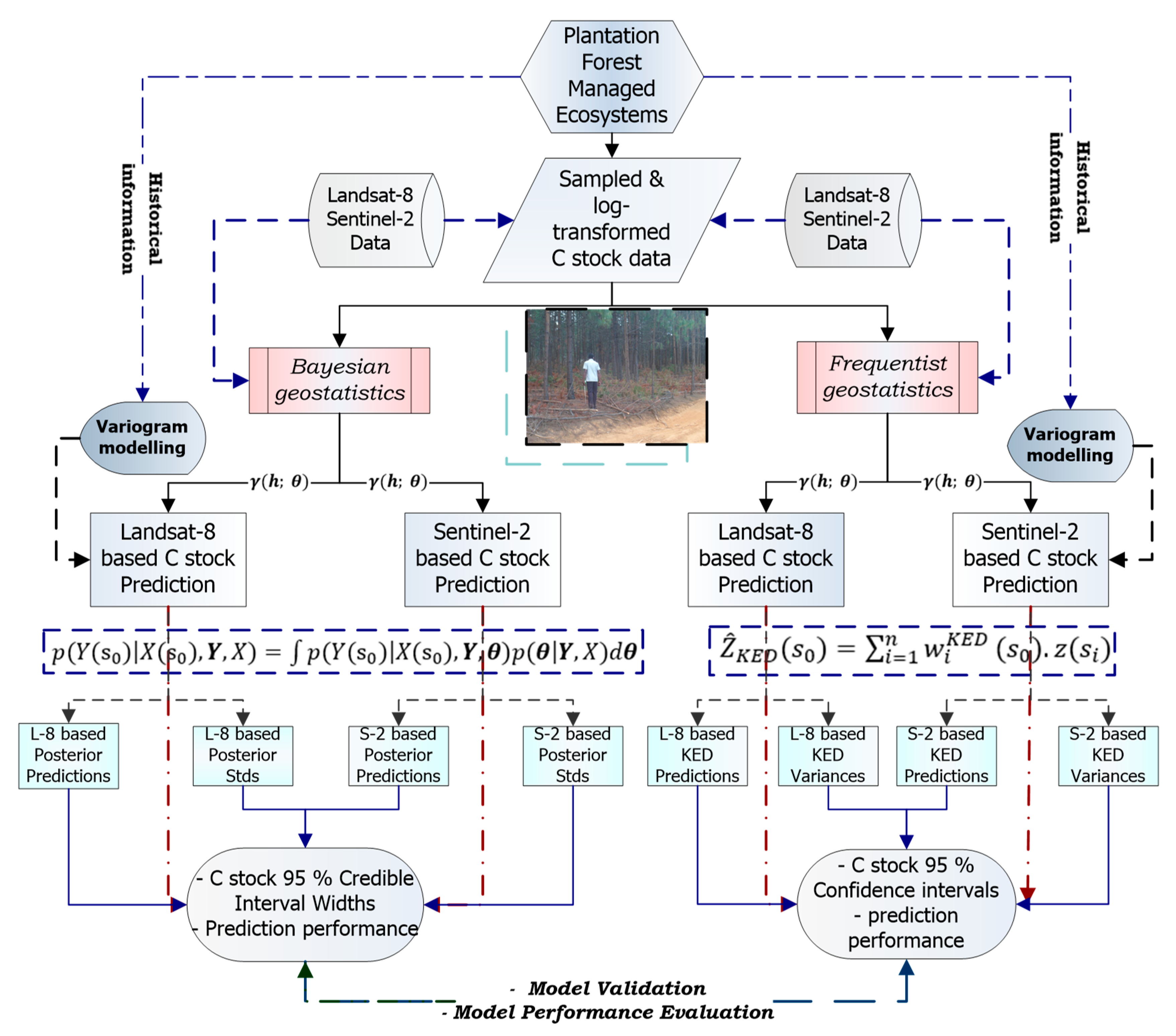
2. Methods
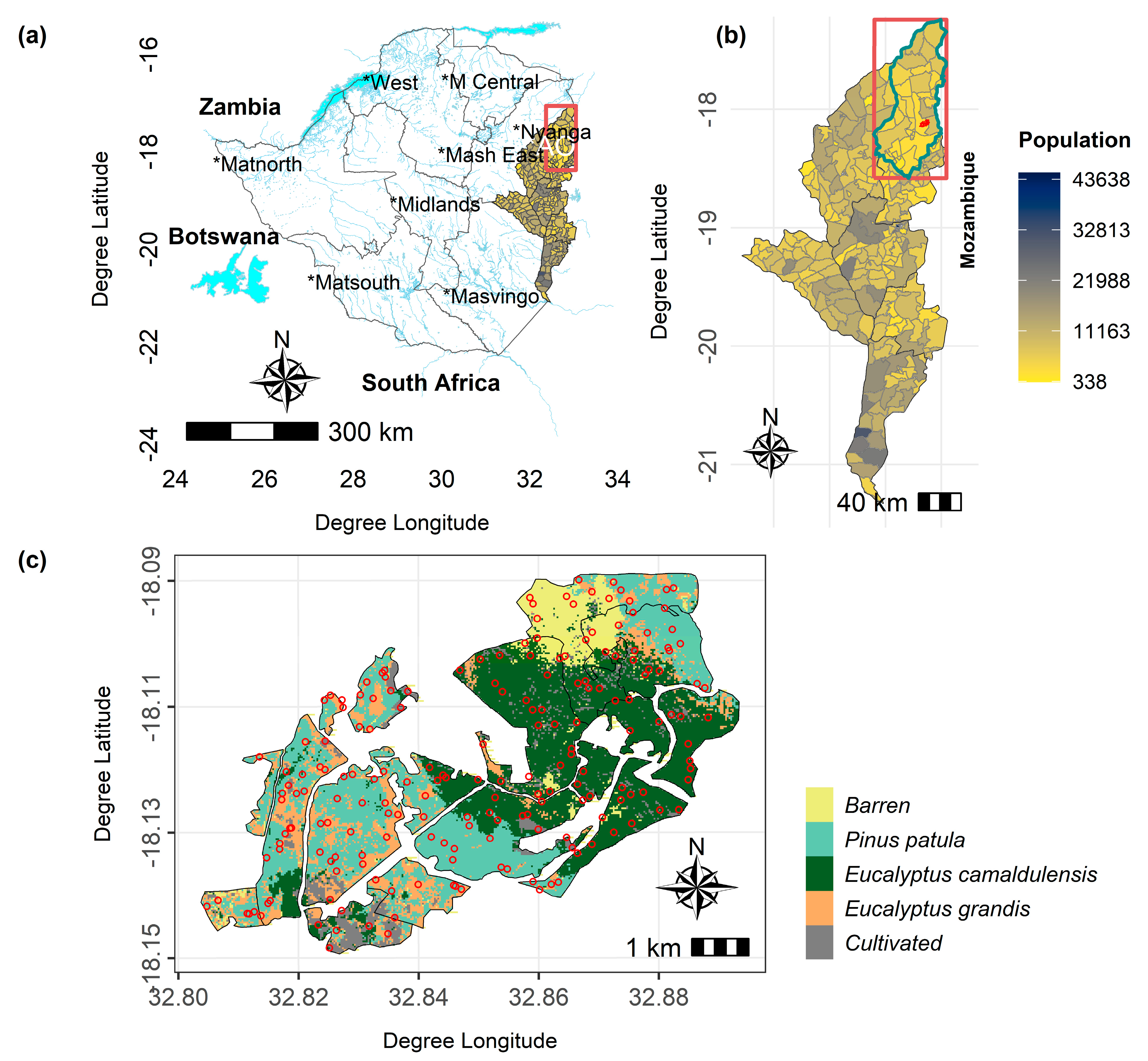
2.1. Study Area
2.2. Remote Sensing Covariates
Landsat OLI and Sentinel-2 MSI Imagery
2.3. Sampling Design
Spatial Coverage Sampling and Mapping of Regionalised Variables
2.4. Carbon Stock Data
2.4.1. Aboveground Tree Biomass (AGTB) Field Measurement
2.4.2. Biomass Calculation and Derivation of C Stock
2.5. The Bayesian Geostatistical Modelling Framework

Bayesian Model Validation and Diagnostic Evaluation
2.6. The Frequentist Geostatistical Modelling Framework
2.6.1. Carbon Stock Spatial Interpolation
2.6.2. Frequentist Model Validation and Diagnostics
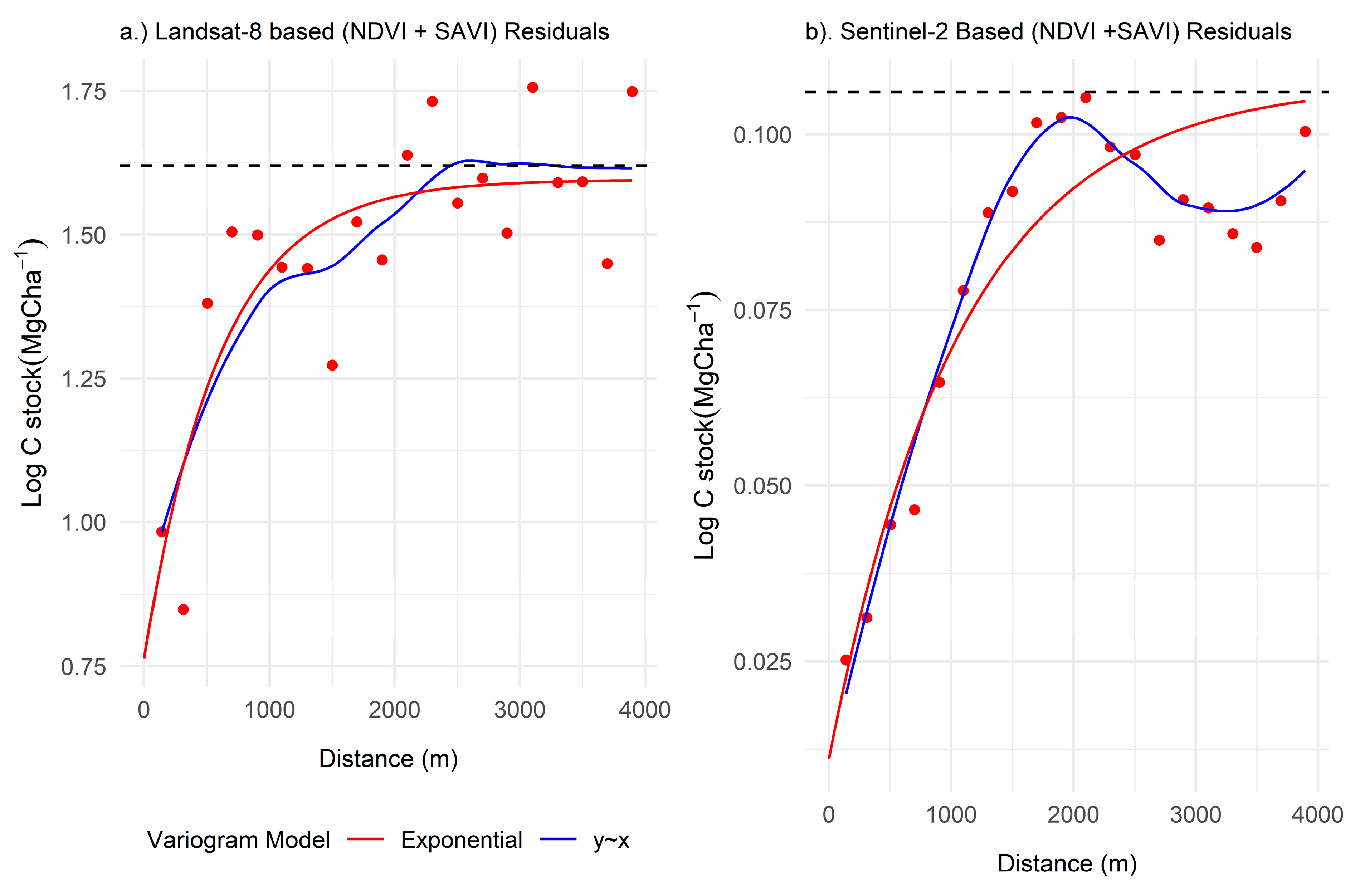
2.7. Variogram Modelling of the Regionalised Variable
3. Results
3.1. C Stock Descriptive Statistics
3.2. Hierarchical Bayesian Geostatistical Approach
3.2.1. C Stock and Medium Resolution Sensor-Derived Vegetation Indices
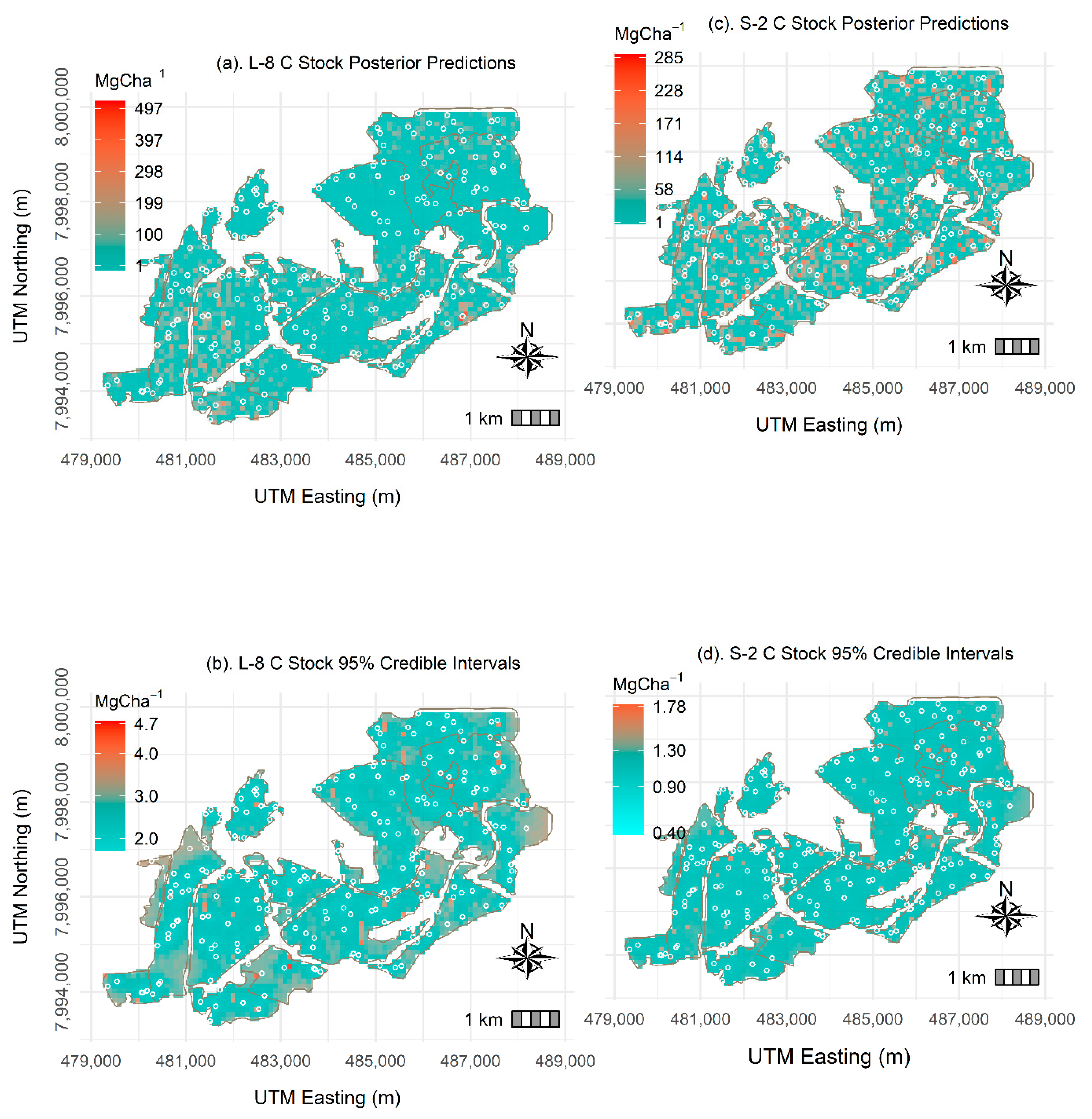
3.2.2. Bayesian-Based C Stock Predictions
3.2.3. Model Validation and Diagnostics
3.3. Frequentist Geostatistical Modelling
3.3.1. C Stock Density
3.3.2. Landsat-8- and Sentinel-2-Based C Stock Linear Modelling
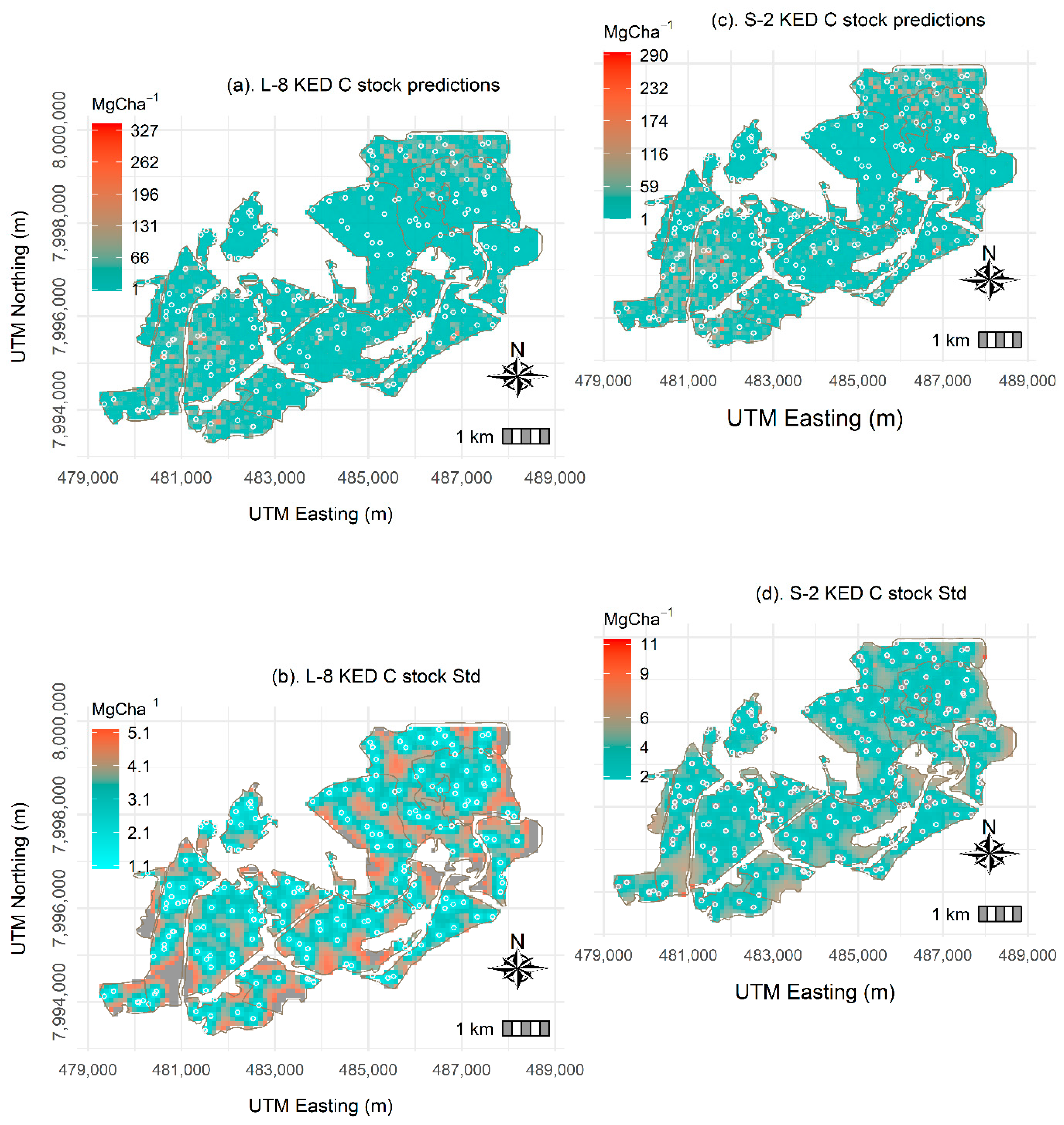
3.3.3. Landsat-8 and Sentinel-2-Based KED Predictions
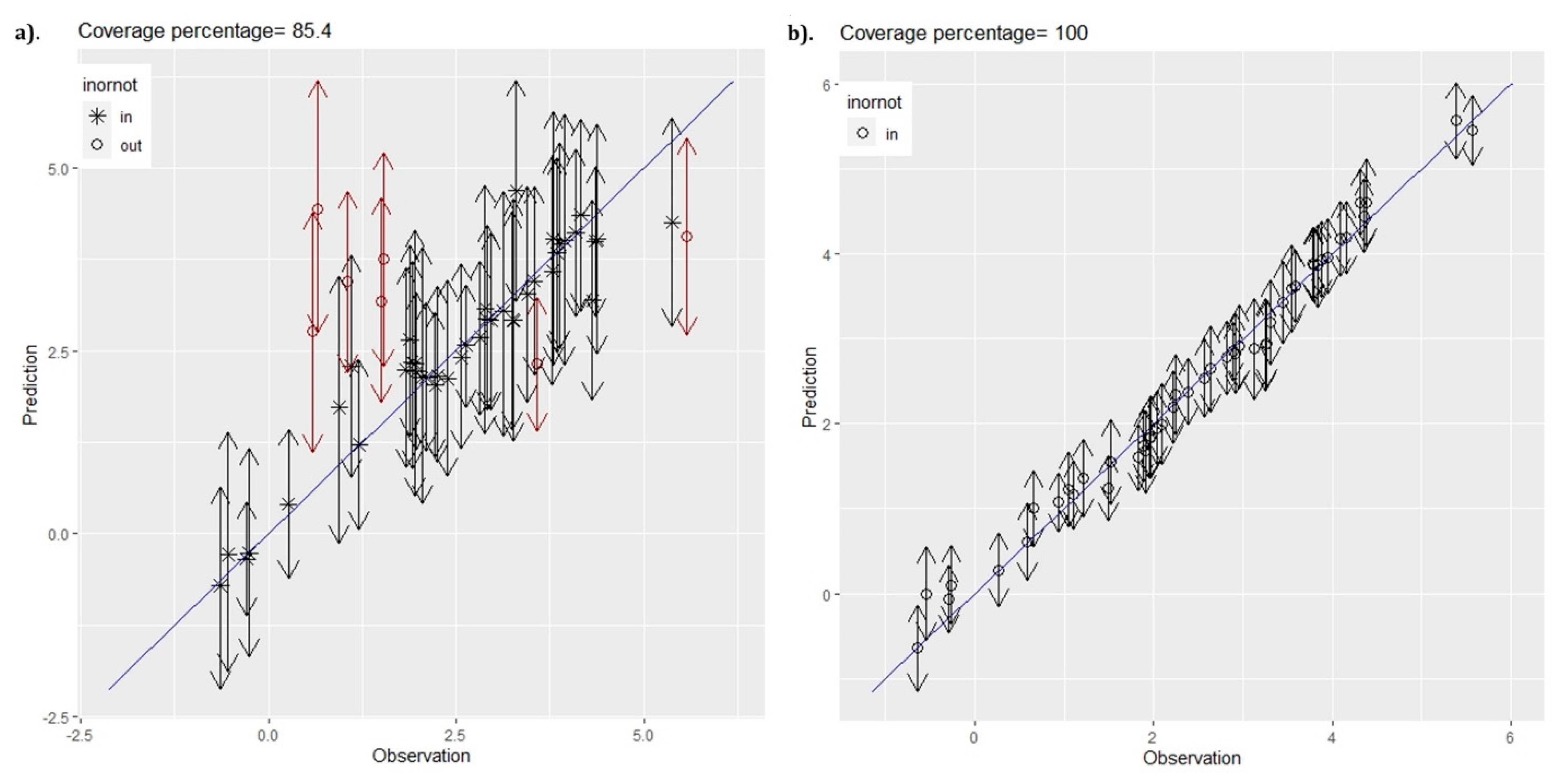
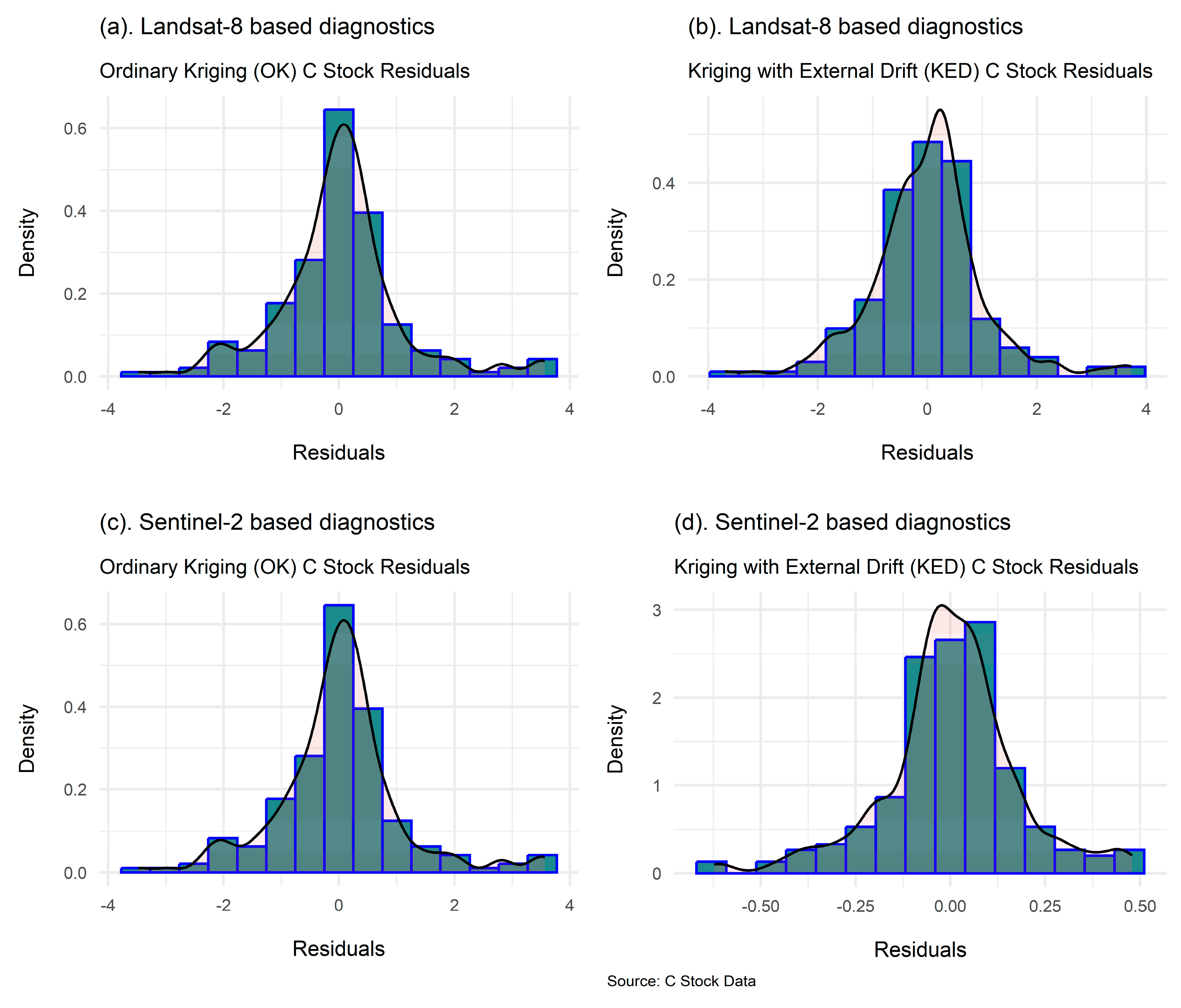
3.3.4. Frequentist Geostatistical Predictive Model Evaluation
3.4. Bayesian- and Frequentist-Based C Stock Predictive Model Summaries
4. Discussion
4.1. Bayesian Geostatistical Approach and C Stock Predictions
4.2. Frequentist Geostatistical Approach and C Stock Predictions
4.3. Comparative Bayesian and Frequentist C Stock Predictive Model Evaluation
5. Conclusions
Author Contributions
Funding
Data Availability Statement
Acknowledgments
Conflicts of Interest
References
- Araki, S.; Yamamoto, K.; Kondo, A. Application of regression kriging to air pollutant concentrations in Japan with high spatial resolution. Aerosol. Air Qual. Res. 2015, 15, 234–241. [Google Scholar] [CrossRef]
- Shoko, C.; Gara, T. Remote sensing of aboveground grass biomass between protected and non-protected areas in savannah rangelands. Afr. J. Ecol. 2021, 59, 687–695. [Google Scholar] [CrossRef]
- Gibbs, H.K.; Brown, S.; Niles, J.O.; Foley, J.A. Monitoring and estimating tropical forest carbon stocks: Making REDD a reality. Environ. Res. Lett. 2007, 2, 45023. [Google Scholar] [CrossRef]
- Van Amstel, A. IPCC 2006 Guidelines for National Greenhouse Gas Inventories. 2006. Available online: https://www.ipcc-nggip.iges.or.jp/public/2006gl/ (accessed on 13 February 2023).
- European-Commission. Timber Trade Flows within, to and from Eastern and Southern African Countries; European-Commission: Brussels, Belgium, 2017. [Google Scholar]
- Government of Zimbabwe. Zimbabwe Revised Nationally Determined Contribution. 2021. Available online: https://unfccc.int/sites/default/files/NDC/2022-06/Zimbabwe%20Revised%20Nationally%20Determined%20Contribution%202021%20Final.pdf (accessed on 13 February 2023).
- Brown, S. Estimating biomass and biomass change of tropical forests: A primer. FAO For. Pap. 1997, 134. [Google Scholar]
- Initiative For Climate Action Transparency (ICAT). Zimbabwe on Track to Better Climate Action Transparency. 2022. Available online: https://climateactiontransparency.org/zimbabwe-on-track-to-better-climate-action-transparency/ (accessed on 28 December 2022).
- Shi, L.; Liu, S. Methods of Estimating Forest Biomass: A Review; Tumuluru, J.S., Ed.; IntechOpen: Rijeka, Croatia, 2017; Chapter 2. [Google Scholar]
- Gelman, A.; John, B.C.; Hals, S.S.; Rubin, D.B. Bayesian Data Analysis, 2nd ed.; Chapman and Hall/CRC: London, UK, 2004. [Google Scholar]
- Cameletti, M.; Biondi, F. Hierarchical modeling of space-time dendroclimatic fields: Comparing a frequentist and a Bayesian approach. Arct. Antarct. Alp. Res. 2019, 51, 115–127. [Google Scholar] [CrossRef]
- Ghosh, G.; Carriazo, F. Bayesian and Frequentist Approaches to Hedonic Modeling in a Geo-Statistical Framework; Agricultural and Applied Economics Association (AAEA): San Antonio, TX, USA, 2007. [Google Scholar]
- Finley, A.O.; Banerjee, S.; McRoberts, R.E. A Bayesian approach to multi-source forest area estimation. Environ. Ecol. Stat. 2008, 15, 241–258. [Google Scholar] [CrossRef]
- Babcock, C.; Finley, A.O.; Bradford, J.B.; Kolka, R.; Birdsey, R.; Ryan, M.G. LiDAR based prediction of forest biomass using hierarchical models with spatially varying coefficients. Remote Sens. Environ. 2015, 169, 113–127. [Google Scholar] [CrossRef]
- Green, E.J.; Finley, A.O.; Strawderman, W.E. Introduction to Bayesian Methods in Ecology and Natural Resources; Springer: Cham, Switzerland, 2020. [Google Scholar]
- Chinembiri, T.S.; Mutanga, O.; Dube, T. Hierarchical Bayesian geostatistics for C stock prediction in disturbed plantation forest in Zimbabwe. Ecol. Inform. 2023, 73, 101934. [Google Scholar] [CrossRef]
- Do, A.N.T.; Tran, H.D.; Ashley, M.; Nguyen, A.T. Monitoring landscape fragmentation and aboveground biomass estimation in Can Gio mangrove biosphere reserve over the past 20 years. Ecol. Inform. 2022, 70, 101743. [Google Scholar] [CrossRef]
- Hudson, G.; Wackernagel, H. Mapping temperature using kriging with external drift: Theory and an example from scotland. Int. J. Climatol. 1994, 14, 77–91. [Google Scholar] [CrossRef]
- Wheeler, D.C.; Waller, L.A. Comparing spatially varying coefficient models: A case study examining violent crime rates and their relationships to alcohol outlets and illegal drug arrests. J. Geogr. Syst. 2009, 11, 1–22. [Google Scholar] [CrossRef]
- Sales, M.H.; Souza, C.M.; Kyriakidis, P.C.; Roberts, D.A.; Vidal, E. Improving spatial distribution estimation of forest biomass with geostatistics: A case study for Rondônia, Brazil. Ecol. Modell. 2007, 205, 221–230. [Google Scholar] [CrossRef]
- Jiang, F.; Sun, H.; Chen, E.; Wang, T.; Cao, Y.; Liu, Q. Above-ground biomass estimation for coniferous forests in Northern China using regression kriging and landsat 9 images. Remote Sens. 2022, 14, 5734. [Google Scholar] [CrossRef]
- Wai, P.; Su, H.; Li, M. Estimating aboveground biomass of two different forest types in myanmar from sentinel-2 data with machine learning and geostatistical algorithms. Remote Sens. 2022, 14, 2146. [Google Scholar] [CrossRef]
- Korhonen, L.; Hadi; Packalen, P.; Rautiainen, M. Comparison of sentinel-2 and landsat 8 in the estimation of boreal forest canopy cover and leaf area index. Remote Sens. Environ. 2017, 195, 259–274. [Google Scholar] [CrossRef]
- Astola, H.; Häme, T.; Sirro, L.; Molinier, M.; Kilpi, J. Comparison of sentinel-2 and landsat 8 imagery for forest variable prediction in boreal region. Remote Sens. Environ. 2019, 223, 257–273. [Google Scholar] [CrossRef]
- Jha, N.; Tripathi, N.K.; Barbier, N.; Virdis, S.G.P.; Chanthorn, W.; Viennois, G.; Brockelman, W.Y.; Nathalang, A.; Tongsima, S.; Sasaki, N.; et al. The real potential of current passive satellite data to map aboveground biomass in tropical forests. Remote Sens. Ecol. Conserv. 2021, 7, 504–520. [Google Scholar] [CrossRef]
- Finley, A.O.; Banerjee, S.; McRoberts, R.E. Hierarchical spatial models for predicting tree species assemblages across large domains. Ann. Appl. Stat. 2009, 3, 1052–1079. [Google Scholar] [CrossRef]
- Banerjee, S.; Finley, A.O.; Waldmann, P.; Ericsson, T. Hierarchical spatial process models for multiple traits in large genetic trials. J. Am. Stat. Assoc. 2010, 105, 506–521. [Google Scholar] [CrossRef]
- Babcock, C.; Finley, A.O.; Andersen, H.-E.; Pattison, R.; Cook, B.D.; Morton, D.C.; Alonzo, M.; Nelson, R.; Gregoire, T.; Ene, L.; et al. Geostatistical estimation of forest biomass in interior Alaska combining landsat-derived tree cover, sampled airborne lidar and field observations. Remote Sens. Environ. 2018, 212, 212–230. [Google Scholar] [CrossRef]
- Neyman, J. Outline of a theory of statistical estimation based on the classical theory of probability. Philos. Trans. R. Soc. A 1937, 236, 333–380. [Google Scholar] [CrossRef]
- Murphy, K.P. A Probabilistic Perspective. Text B. 2012. Available online: https://d1wqtxts1xzle7.cloudfront.net/55735470/Machine_learning_A_Probabilistic_Perspective.pdf?1517974187=&response-content-disposition=inline%3B+filename%3DMachine_Learning_A_Probabilistic_Perspec.pdf&Expires=1679287483&Signature=SEV-l8rcLLC3o8k0iRZX9fOoWoZyp82ssxglfGtk0vQxpatA4vLCM8nN-HADoVT8IzBf631g3xykOibpqa4vc2nNoievSdbei8VU-xjSNRe0cS0w6r58QVkyRnmE7tgpLWh8-6dRDE-x-x88aY84sbUQQOxIgzn1ZjIQT2ifMVBRXogQHsYEtdp04qL5umm-KJ9iqeyV3SpZO0rLLEaXArtn6ALLV2PXVBy-uWeLAWsvMloCuxxXAIyoCSHaf32VWrL8tICMlM2bvMWW0r62FtRbd1d7jz3dNvL-ENGFXJOOgFjrjBwGY~Xa3u2QNBjcTsTVMRn-M9LL7AjPf9oNUQ__&Key-Pair-Id=APKAJLOHF5GGSLRBV4ZA (accessed on 13 February 2023).
- Hazra, A. Using the confidence interval confidently. J. Thorac. Dis. 2017, 9, 4124–4129. [Google Scholar] [CrossRef]
- Edwards, W.; Lindman, H.; Savage, L.J. Bayesian statistical inference for psychological research. Psychol. Rev. 1963, 70, 193–242. [Google Scholar] [CrossRef]
- Box, G.E.P.; Tiao, G.C. Bayesian Inference in Statistical Analysis; Wiley: New York, NY, USA, 1992. [Google Scholar]
- Goulard, M.; Voltz, M. Linear coregionalization model: Tools for estimation and choice of cross-variogram matrix. Math. Geol. 1992, 24, 269–286. [Google Scholar] [CrossRef]
- Forestry-Commission. Zimbabwe Land and Vegetation Cover Area Estimates; Forestry-Commission: Harare, Zimbabwe, 2021. [Google Scholar]
- Zvobgo, L.; Tsoka, J. Deforestation rate and causes in upper manyame sub-catchment, Zimbabwe: Implications on achieving national climate change mitigation targets. Trees For. People 2021, 5, 100090. [Google Scholar] [CrossRef]
- Whitlow, T. Land Degradation in Zimbabwe. A Geographical Study; University of Zimbabwe (UZ): Harare, Zimbabwe, 1998. [Google Scholar]
- FAO. Forestry Outlook Study for Africa. Regional Report—Opportunities and Challenges towards 2020; FAO: Rome, Italy, 2003. [Google Scholar]
- Drusch, M.; Del Bello, U.; Carlier, S.; Colin, O.; Fernandez, V.; Gascon, F.; Hoersch, B.; Isola, C.; Laberinti, P.; Martimort, P.; et al. Sentinel-2: ESA’s optical high-resolution mission for GMES operational services. Remote Sens. Environ. 2012, 120, 25–36. [Google Scholar] [CrossRef]
- Frampton, W.J.; Dash, J.; Watmough, G.; Milton, E.J. Evaluating the capabilities of sentinel-2 for quantitative estimation of biophysical variables in vegetation. ISPRS J. Photogramm. Remote Sens. 2013, 82, 83–92. [Google Scholar] [CrossRef]
- Ranghetti, L.; Boschetti, M.; Nutini, F.; Busetto, L. ‘sen2r’: An R toolbox for automatically downloading and preprocessing sentinel-2 satellite data. Comput. Geosci. 2020, 139, 104473. [Google Scholar] [CrossRef]
- Walvoort, D.; Brus, D.; de Gruijter, J. An R package for spatial coverage sampling and random sampling from compact geographical strata by k-means. Comput. Geosci. 2010, 36, 1261–1267. [Google Scholar] [CrossRef]
- Brus, D.; de Gruijter, J.; van Groenigen, J. Chapter 14 designing spatial coverage samples using the k-means clustering algorithm. Dev. Soil Sci. 2006, 31, 183–192. [Google Scholar]
- Li, C.; Li, X. Hazard rate and reversed hazard rate orders on extremes of heterogeneous and dependent random variables. Stat. Probab. Lett. 2019, 146, 104–111. [Google Scholar] [CrossRef]
- Bordoloi, R.; Das, B.; Tripathi, O.; Sahoo, U.; Nath, A.; Deb, S.; Das, D.; Gupta, A.; Devi, N.; Charturvedi, S.; et al. Satellite based integrated approaches to modelling spatial carbon stock and carbon sequestration potential of different land uses of Northeast India. Environ. Sustain. Indic. 2022, 13, 100166. [Google Scholar] [CrossRef]
- Ravindranath, N.H.; Ostwald, M. Carbon inventory methods handbook for greenhouse gas inventory, carbon mitigation and roundwood production projects. Adv. Glob. Chang. Res. Vol. 2008, 29. [Google Scholar] [CrossRef]
- Zunguze, A.X. Quantificação de Carbono Sequestrado em Povoamentos de Eucalyptus Spp na Floresta de Inhamacari-Manica; Universidade Eduardo Mondlane: Maputo, Mozambique, 2012. [Google Scholar]
- Finley, A.O.; Banerjee, S.; MacFarlane, D.W. A hierarchical model for quantifying forest variables over large heterogeneous landscapes with uncertain forest areas. J. Am. Stat. Assoc. 2011, 106, 31–48. [Google Scholar] [CrossRef]
- Finley, A.; Sudipto, B.; Carlin, B. spBayes: An R package for univariate and multivariate hierarchical point-referenced spatial models. J. Stat. Softw. 2007, 19. [Google Scholar] [CrossRef]
- R Core Development, T. A Language and Environment for Statistical Computing; R Foundation for Statistical Computing: Vienna, Austria, 2008. [Google Scholar]
- Gelfand, A.E. Hierarchical modeling for spatial data problems. Spat. Stat. 2012, 1, 30–39. [Google Scholar] [CrossRef]
- Demirhan, H.; Kalaylioglu, Z. Joint prior distributions for variance parameters in Bayesian analysis of normal hierarchical models. J. Multivar. Anal. 2015, 135, 163–174. [Google Scholar] [CrossRef]
- Duchêne, S.; Duchêne, D.A.; Di Giallonardo, F.; Eden, J.-S.; Geoghegan, J.L.; Holt, K.E.; Ho, S.Y.W.; Holmes, E.C. Cross-validation to select Bayesian hierarchical models in phylogenetics. BMC Evol. Biol. 2016, 16, 115. [Google Scholar] [CrossRef]
- Spiegelhalter, D.J.; Best, N.G.; Carlin, B.P.; Van Der Linde, A. Bayesian measures of model complexity and fit. J. R. Stat. Soc. Ser. B Stat. Methodol. 2002, 64, 583–639. [Google Scholar] [CrossRef]
- Jackman, S. Estimation and inference via bayesian simulation: An introduction to markov chain monte carlo. Am. J. Pol. Sci. 2000, 44, 375–404. [Google Scholar] [CrossRef]
- Odeh, I.O.A.; McBratney, A.B.; Chittleborough, D.J. Further results on prediction of soil properties from terrain attributes: Heterotopic cokriging and regression-kriging. Geoderma 1995, 67, 215–226. [Google Scholar] [CrossRef]
- Kupfersberger, H.; Deutsch, C.V.; Journel, A.G. Deriving constraints on small-scale variograms due to variograms of large-scale data. Math. Geol. 1998, 30, 837–852. [Google Scholar] [CrossRef]
- Hengl, T.; Walvoort, D.J.J.; Brown†, A.; Rossiter, D.G. A double continuous approach to visualization and analysis of categorical maps. Int. J. Geogr. Inf. Sci. 2004, 18, 183–202. [Google Scholar] [CrossRef]
- Webster, R.; Welham, S.J.; Potts, J.M.; Oliver, M.A. Estimating the spatial scales of regionalized variables by nested sampling, hierarchical analysis of variance and residual maximum likelihood. Comput. Geosci. 2006, 32, 1320–1333. [Google Scholar] [CrossRef]
- Stoyan, D. Statistical Analysis of Spatial and Spatio-Temporal Point Patterns, 3rd ed.; CRC Press: New York, NY, USA. [CrossRef]
- Sahu, S.K. Bayesian Modeling of Spatio Temporal Data with R, 1st ed.; Chapman and Hall/CRC: Southampton, UK, 2022. [Google Scholar]
- Pascual, A.; Tupinambá-Simões, F.; de Conto, T. Using multi-temporal tree inventory data in eucalypt forestry to benchmark global high-resolution canopy height models. A showcase in Mato Grosso, Brazil. Ecol. Inform. 2022, 70, 101748. [Google Scholar] [CrossRef]
- Box, G.E.P.; Cox, D.R. An analysis of transformations revisited, rebutted. J. Am. Stat. Assoc. 1982, 77, 209–210. [Google Scholar] [CrossRef]
- El-Askary, H.; Abd El-Mawla, S.H.; Li, J.; El-Hattab, M.M.; El-Raey, M. Change detection of coral reef habitat using Landsat-5 TM, Landsat 7 ETM+ and Landsat 8 OLI data in the Red Sea (Hurghada, Egypt). Int. J. Remote Sens. 2014, 35, 2327–2346. [Google Scholar] [CrossRef]
- Jia, K.; Wei, X.; Gu, X.; Yao, Y.; Xie, X.; Li, B. Land cover classification using landsat 8 operational land imager data in Beijing, China. Geocarto Int. 2014, 29, 941–951. [Google Scholar] [CrossRef]
- Isaaks, E.H.; Srivastava, R.M. Applied Geostatistics; Oxford University Press: Oxford, UK, 1989. [Google Scholar]
- Diggle, P.; Ribeiro, P.J. Model-Based Geostatistics. J. R. Stat. Soc. C 2007, 846, 15–27. [Google Scholar]
- Baloloy, A.B.; Blanco, A.; Candido, C.G.; Argamosa, R.J.L.; Dumalag, J.B.L.C.; Dimapilis, L.L.C.; Paringit, E. Estimation of mangrove forest aboveground biomass using multispectral bands, vegetation indices and biophysical variables derived from optical satellite imageries: Rapideye, planetscope and sentinel-2. ISPRS Ann. Photogramm. Remote Sens. Spat. Inf. Sci. 2018, IV-3, 29–36. [Google Scholar] [CrossRef]
- Sovdat, B.; Kadunc, M.; Batič, M.; Milčinski, G. Natural color representation of Sentinel-2 data. Remote Sens. Environ. 2019, 225, 392–402. [Google Scholar] [CrossRef]
- Wang, Q.; Li, J.; Jin, T.; Chang, X.; Zhu, Y.; Li, Y.; Sun, J.; Li, D. Comparative analysis of landsat-8, sentinel-2, and GF-1 data for retrieving soil moisture over wheat farmlands. Remote Sens. 2020, 12, 2708. [Google Scholar] [CrossRef]
- Jiang, F.; Kutia, M.; Ma, K.; Chen, S.; Long, J.; Sun, H. Estimating the aboveground biomass of coniferous forest in Northeast China using spectral variables, land surface temperature and soil moisture. Sci. Total Environ. 2021, 785, 147335. [Google Scholar] [CrossRef] [PubMed]
- Dang, A.T.N.; Nandy, S.; Srinet, R.; Luong, N.V.; Ghosh, S.; Senthil Kumar, A. Forest aboveground biomass estimation using machine learning regression algorithm in Yok Don National Park, Vietnam. Ecol. Inform. 2019, 50, 24–32. [Google Scholar] [CrossRef]
- Takagi, K.; Yone, Y.; Takahashi, H.; Sakai, R.; Hojyo, H.; Kamiura, T.; Nomura, M.; Liang, N.; Fukazawa, T.; Miya, H.; et al. Forest biomass and volume estimation using airborne LiDAR in a cool-temperate forest of northern Hokkaido, Japan. Ecol. Inform. 2015, 26, 54–60. [Google Scholar] [CrossRef]
- Kramer, C.Y. Extension of multiple range tests to group means with unequal numbers of replications. Biometrics 1956, 12, 307–310. [Google Scholar] [CrossRef]
- Chinembiri, T.S.; Bronsveld, M.C.; Rossiter, D.G.; Dube, T. The precision of C stock estimation in the ludhikola watershed using model-based and design-based approaches. Nat. Resour. Res. 2013, 22, 297–309. [Google Scholar] [CrossRef]
- Tveito, O.E.; Wegehenkel, M.; van der Wel, F. The use of geographic information systems in climatology and meteorology. SAGE 2003, 27. [Google Scholar] [CrossRef]
- Gupta, A.; Kamble, T.; Machiwal, D. Comparison of ordinary and Bayesian kriging techniques in depicting rainfall variability in arid and semi-arid regions of north-west India. Environ. Earth Sci. 2017, 76, 512. [Google Scholar] [CrossRef]
- Dube, T.; Mutanga, O. Evaluating the utility of the medium-spatial resolution Landsat 8 multispectral sensor in quantifying aboveground biomass in uMgeni catchment, South Africa. ISPRS J. Photogramm. Remote Sens. 2015, 101, 36–46. [Google Scholar] [CrossRef]
- Li, S.; Ganguly, S.; Dungan, J.L.; Wang, W.; Nemani, R.R. Sentinel-2 MSI radiometric characterization and cross-calibration with landsat-8 OLI. Adv. Remote Sens. 2017, 6, 147–159. [Google Scholar] [CrossRef]
- Ver Hoef, J. Sampling and geostatistics for spatial data. Écoscience 2002, 9, 152–161. [Google Scholar] [CrossRef]
- Babcock, C.; Finley, A.O.; Cook, B.D.; Weiskittel, A.; Woodall, C.W. Modeling forest biomass and growth: Coupling long-term inventory and LiDAR data. Remote Sens. Environ. 2016, 182, 1–12. [Google Scholar] [CrossRef]
- FAO. Global Forest Resources Assessment Country Report, Zimbabwe; FAO: Rome, Italy, 2005. [Google Scholar]
- Wu, C.; Shen, H.; Shen, A.; Deng, J.; Gan, M.; Zhu, J.; Xu, H.; Wang, K. Comparison of machine-learning methods for above-ground biomass estimation based on Landsat imagery. J. Appl. Remote Sens. 2016, 10, 35010. [Google Scholar] [CrossRef]
- Xiong, Y.; Wang, H. Spatial relationships between NDVI and topographic factors at multiple scales in a watershed of the Minjiang River, China. Ecol. Inform. 2022, 69, 101617. [Google Scholar] [CrossRef]
- Meyer, H.L.; Marco, H.; Burkhard, B.; Joseph, P.; Dirk, P. Comparison of landsat-8 and sentinel-2 data for estimation of leaf area index in temperate forests. Remote Sens. 2019, 11, 1160. [Google Scholar] [CrossRef]


| Statistic (MgCha−1) | Eucalyptus camaldulensis | Eucalyptus grandis | Pinus patula | ||||||
|---|---|---|---|---|---|---|---|---|---|
| DBH | Height | C Stock | DBH | Height | C Stock | DBH | Height | C Stock | |
| 81.4 | 60.6 | 2485.3 | 67.4 | 70.6 | 405.7 | 56.8 | 58.6 | 377.9 | |
| 77.4 | 52.7 | 1470.3 | 51.4 | 49.7 | 327.8 | 43.5 | 38.7 | 295.4 | |
| 231.9 | 88.9 | 8998.2 | 97.9 | 90.1 | 429.8 | 64.3 | 66.6 | 600.3 | |
| 11.4 | 23.8 | 13.7 | 14.7 | 27.8 | 111.3 | 10.6 | 19.4 | 9.7 | |
| n | 97 | - | - | 60 | - | - | 34 | - | - |
| s.td | 57.6 | - | - | 51.7 | - | - | 48.9 | - | - |
| Parameter | Landsat-8 OLI C Stock Model | Sentinel-2 MSI C Stock Model | ||||||
|---|---|---|---|---|---|---|---|---|
| Mean | s.d | 2.5% | 97.5% | Mean | s.d | 2.5% | 97.5% | |
| 1.34 | 0.49 | 0.37 | 2.27 | 0.93 | 0.24 | 1.42 | −0.49 | |
| 4.49 | 0.94 | 2.63 | 6.30 | 6.30 | 0.11 | 6.06 | 6.51 | |
| −0.50 | 0.72 | −1.55 | 1.26 | 0.02 | 0.38 | −0.72 | 0.77 | |
| −0.50 | 0.55 | −1.65 | 0.53 | 0.01 | 0.11 | −0.19 | 0.22 | |
| 1.47 | 0.39 | 0.76 | 2.22 | 0.07 | 0.01 | 0.053 | 0.10 | |
| 0.39 | 0.15 | 0.13 | 0.68 | 0.005 | 0.004 | 0.0005 | 0.01 | |
| 0.0013 | 0.000 | 0.0013 | 0.0014 | 0.0012 | 0.0003 | 0.0014 | 0.0023 | |
| Model Evaluation Criterion | Landsat-8-Derived Predictors | Sentinel-2-Derived Predictors | ||||
|---|---|---|---|---|---|---|
| Independent Error Model | Spatial Intercept Only Model | Spatial Model | Independent Error Model | Spatial Intercept Only Model | Spatial Model | |
| (Mgha−1) | 1.23 | 0.97 | 0.97 | 0.31 | 1.18 | 0.17 |
| (Mgha−1) | 0.93 | 0.53 | 0.57 | 0.26 | 0.77 | 0.13 |
| (Mgha−1) | 0.72 | 0.38 | 0.38 | 0.20 | 0.56 | 0.14 |
| (%) | 91.67 | 85.42 | 85.42 | 95.83 | 89.58 | 100.00 |
| 220.8 | 48.40 | 71.0 | −201.3 | 283.5 | −564.5 | |
| Predictors | Landsat-8-Based Linear Model | Sentinel-2-Based Linear Model | ||||
|---|---|---|---|---|---|---|
| Coefficient | p-Value | Coefficient | p-Value | |||
| 0.03 | 0.93 | Insignificant | −0.30 | 0.31 | Insignificant | |
| 7.67 | 0.00 | Significant | 6.69 | 0.00 | Significant | |
| 1.04 | 0.11 | Insignificant | 1.24 | 0.01 | Significant | |
| 0.33 | 0.57 | Insignificant | 0.20 | 0.15 | Insignificant | |
| Predictors | Landsat-8-Based C Stock Predictions | Sentinel-2-Based C Stock Predictions | ||
|---|---|---|---|---|
| Ordinary Kriging (OK) | Kriging with External Drift (KED) | Ordinary Kriging (OK) | Kriging with External Drift (KED) | |
| 1.01 | 1.00 | 1.01 | 1.00 | |
| 1.01 | 1.00 | 1.01 | 1.00 | |
| 2.94 | 2.84 | 2.91 | 1.19 | |
| 222.34 | 208.42 | 222.34 | 6.06 | |
| Modelling Approach | Test Statistic | p-Value | Modelling Technique |
|---|---|---|---|
| Frequentist approach | 0.097 | 0.264 | Landsat-8 |
| Frequentist approach | 0.132 | 0.136 | Landsat-8 |
| Hierarchical Bayesian approach | 0.975 | 0.367 | Sentinel-2 |
| Hierarchical Bayesian approach | 0.773 | 0.278 | Sentinel-2 |
| Validation Criterion | Bayesian Geostatistical Approach | Frequentist Geostatistical Approach | ||
|---|---|---|---|---|
| Landsat-8-Based C Stock Model | Sentinel-2-Based C Stock Model | Landsat-8-Based C Stock Model | Sentinel-2-Based C Stock Model | |
| RMSE | 0.97 | 0.17 | 2.84 | 1.19 |
| ME | 0.57 | 0.13 | 1.01 | 1.00 |
| Error/CIWs | ||||
| Prediction range | ||||
| Conclusion | Overprediction | Perfect | Overprediction | Perfect |
Disclaimer/Publisher’s Note: The statements, opinions and data contained in all publications are solely those of the individual author(s) and contributor(s) and not of MDPI and/or the editor(s). MDPI and/or the editor(s) disclaim responsibility for any injury to people or property resulting from any ideas, methods, instructions or products referred to in the content. |
© 2023 by the authors. Licensee MDPI, Basel, Switzerland. This article is an open access article distributed under the terms and conditions of the Creative Commons Attribution (CC BY) license (https://creativecommons.org/licenses/by/4.0/).
Share and Cite
Chinembiri, T.S.; Mutanga, O.; Dube, T. Carbon Stock Prediction in Managed Forest Ecosystems Using Bayesian and Frequentist Geostatistical Techniques and New Generation Remote Sensing Metrics. Remote Sens. 2023, 15, 1649. https://doi.org/10.3390/rs15061649
Chinembiri TS, Mutanga O, Dube T. Carbon Stock Prediction in Managed Forest Ecosystems Using Bayesian and Frequentist Geostatistical Techniques and New Generation Remote Sensing Metrics. Remote Sensing. 2023; 15(6):1649. https://doi.org/10.3390/rs15061649
Chicago/Turabian StyleChinembiri, Tsikai Solomon, Onisimo Mutanga, and Timothy Dube. 2023. "Carbon Stock Prediction in Managed Forest Ecosystems Using Bayesian and Frequentist Geostatistical Techniques and New Generation Remote Sensing Metrics" Remote Sensing 15, no. 6: 1649. https://doi.org/10.3390/rs15061649
APA StyleChinembiri, T. S., Mutanga, O., & Dube, T. (2023). Carbon Stock Prediction in Managed Forest Ecosystems Using Bayesian and Frequentist Geostatistical Techniques and New Generation Remote Sensing Metrics. Remote Sensing, 15(6), 1649. https://doi.org/10.3390/rs15061649