A Comparative Study of the Temperature Change in a Warm Eddy Using Multisource Data

Abstract

An ocean acoustic tomography (OAT) experiment conducted in the northern South China Sea in 2021 measured a month-long record of acoustic travel times along paths of over one hundred kilometers in range. A mesoscale eddy passed through the experimental region during the deployment of four acoustic moorings, providing unique OAT data for examining the deep temperature change in the eddy and for comparison with the Hybrid Coordinate Ocean Model (HYCOM) data. The existence of the eddy is first confirmed by the merged sea level anomaly (MSLA) image and HYCOM data and it can exceed the depth of the sound channel axis. The temperature changes measured by temperature and depth (TD)/conductivity–temperature–depth (CTD) loggers and by the OAT sound speed are in accordance with those reflected on the MSLA image during the movement of the eddy. However, the eddy movement prompted by temperature changes in the HYCOM data is different from that measured by TD/CTD. The modeled eddy intensity is at least two times less than the measured eddy intensity. At the sound channel axis depth, a factor of approximately 4.17 ms⁻¹ °C⁻¹ can be used to scale between sound speed and temperature. The transmission/reception path-averaged temperature of the eddy derived from the OAT-computed sound speed at the depth of the sound channel axis is five times greater than those in the HYCOM data. OAT is feasible as a tool to study mesoscale eddy properties in the deep ocean, while HYCOM data are not accurate enough for this mesoscale eddy at the sound channel axis depth. It is suggested that the model be refined by the OAT path-averaged temperature as constraints when the HYCOM data capture the mesoscale eddies.

1. Introduction

The South China Sea (SCS) is of great oceanographic interest, not only because the internal wave is prevalent throughout the north of the semi-closed oceans [1,2], but also the ocean is full of mesoscale eddies [3,4,5,6]. Mesoscale eddies are capable of carrying water bodies with different characteristics from their surroundings, enabling the transport of oceanic mass and energy, and are an important factor in supporting the oceanic thermohaline circulation, as well as maintaining the oceanic energy scale string [7,8]. At the same time, the hydrodynamic properties of eddies play an important role in providing nutrients, which can affect plankton blooms [9]. The existence of ocean eddies also causes significant changes in the structure of the vertical profile of the sound speed in a certain area, which in turn alters the propagation form of acoustic waves and the energy distribution pattern of the sound field, thus affecting the underwater detection and counter-detection of sonar [10,11,12,13]. Numerous studies show that eddies greatly change the sound field’s main distribution when compared to a sound field without eddies. The eddy causes major changes in the arrival structure captured by a vertical array, e.g., acoustic arrival time perturbations by mesoscale eddies [14]. The presence of the eddy could result in the percentage of energy arriving at angles less than 5° from the broad side from 5% to 50% [15]. The eddy’s position relative to the source induces changes in transmission loss of up to 20 dB [15,16]. The horizontal angle of the ray path is shifted through the eddy, bringing about horizontal deflections in excess of 1° [17,18]. Warm eddies reduce the width of the convergence zone (CZ), while the opposite effect is observed for cold eddies [19]. Propagation across the eddy boundary is shown to create a second series of CZs, in addition to the normal series [20]. All mentioned above constitute the forward problem of ocean acoustics.

Understanding the forward problem is fundamental for addressing any inverse problem. Ocean acoustic tomography (OAT) as an inverse method, first proposed by Munk and Wunsch in 1979 [21], has focused on exploiting the remote sensing capabilities of acoustics using both active (acoustic tomography) and passive sources [22,23,24]. OAT can make a simultaneous mapping of time-varying subsurface structures such as current velocity, water temperature, and sound speed [22,25,26]. Over the years, accurate measurement of the time or other characteristics of acoustic propagation is made to infer oceanic phenomena in the deep region traversed by the sound field [12,27,28,29,30], especially dramatically varying oceanic phenomena (e.g., mesoscale eddies) being a direction of development. However, the exploration of deep-sea mesoscale eddies by OAT is still stuck in reconstructing the frontal boundary shapes of an eddy [12], or lower root mean squared error (RMSE) in the structural estimation of mesoscale eddy [31] or halving the number of coefficients for mesoscale eddy representation [32] or changing the coupling coefficient of different orders of normal modes greatly, without reconstructing three-dimensional eddy profile [30]. There is no definite estimation of the temperature change in a deep-sea mesoscale eddy by the OAT method, which motivates the development of this paper.

Since the significance of SCS eddy in oceanography and acoustics, a warm mesoscale eddy was observed passing through the OAT experimental region in the northern SCS in 2021. Combining acoustic and hydrological moorings, all equipment was placed to be within an area of about 100 km square, and constructed an observation system. The OAT provides unique data for the eddy evolution study while it progresses through the region. The tomography system was usually designed to resolve acoustic signals with O (10 ms) precision [28] and to identify specific ray paths with specific ray arrivals [33]. Individual ray arrivals were not observed in this experiment due to system design deficiencies. Nevertheless, the information from the tomographic measurements is primarily the transmission/reception path-averaged temperature of the eddy derived from the OAT-computed sound speed at the depth of the sound channel axis. This technique can provide a better understanding of the deep-water body where the mesoscale eddy is located and has significant advantages in the observation of eddy deep temperature evolution. To compare the deep temperature change in the warm eddy as it moved over the transmission/reception sections from the OAT data, the Hybrid Coordinate Ocean Model (HYCOM) ocean model, as reference ocean, is employed and compared for the eddy temperature evolution because it has certain advantages in the simulation of the South China Sea [34]. The use of HYCOM ocean models is essential to assess the relative impact of the various data types on the mesoscale eddies estimates. A comparative study of the properties of moored/point, satellite remote sensing, acoustic tomography/integral observations, and ocean models of mesoscale eddy in the 2021 north SCS in this paper provide some data types that are both accurate and complementary to data from other on-going programs.

The purpose of this paper is to convert the tomographic eddy temperature variation estimates of sound speed to temperature estimates and compare it with the temperature variation obtained from HYCOM to fill the gap between the deep-sea temperature variations of actual ocean mesoscale eddy and that obtained by existing models. In Section 2, the experiments and data sources are first described, and then the data how to be processed, including the conversion between sound speed and temperature or salinity and the calculation of the average temperature over the path. The movement of the mesoscale eddy as demonstrated by the merged sea level anomaly (MSLA) and HYCOM is outlined in Section 3, the temperature information of the mesoscale eddy obtained from the OAT experiment is presented in Section 4, and the mesoscale eddy properties obtained from multiple sources are compared in Section 5. Section 6 explains the strengths and limitations of this study. Finally, a concluding discussion is given in Section 7.

2. Data and Methodology

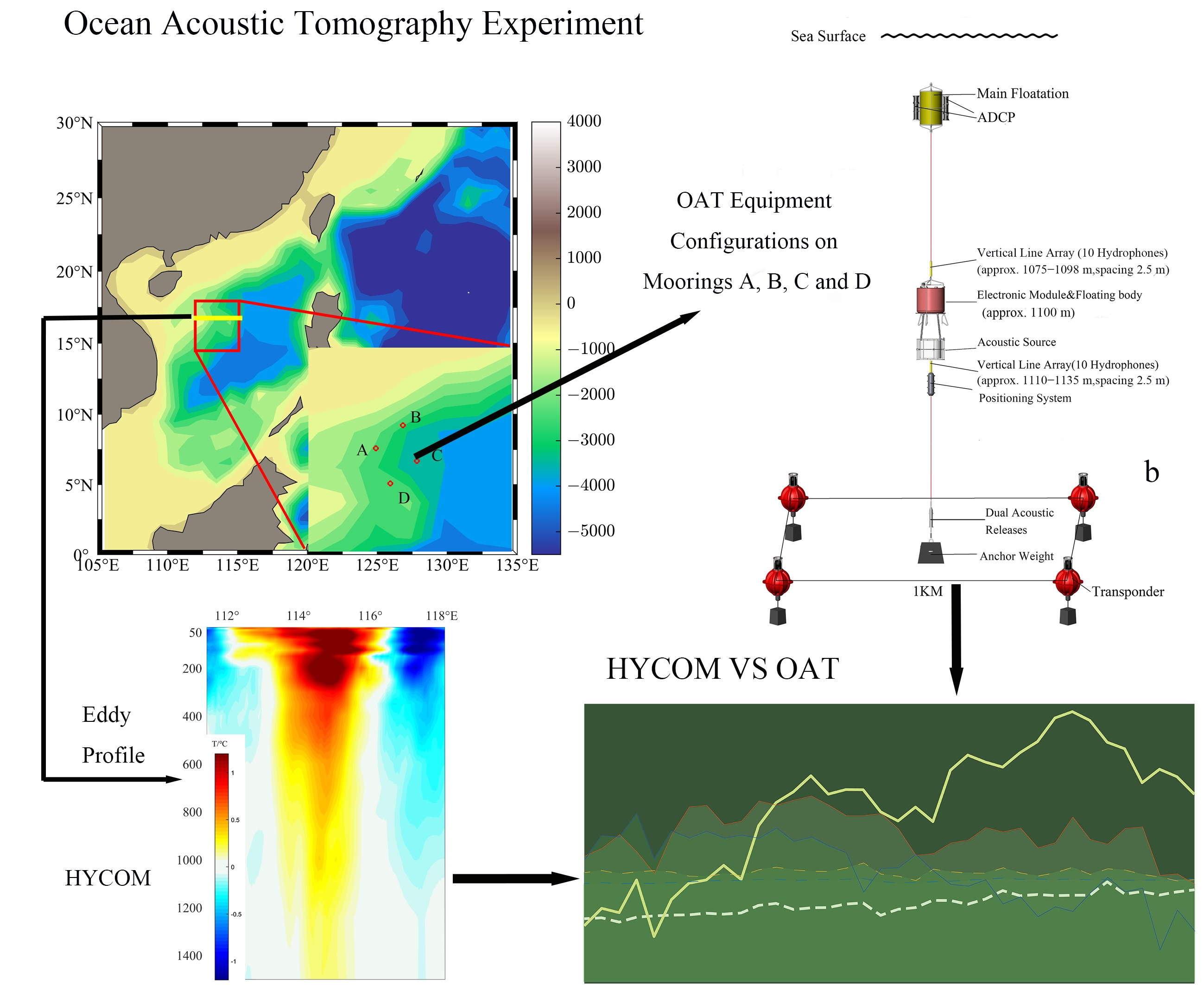
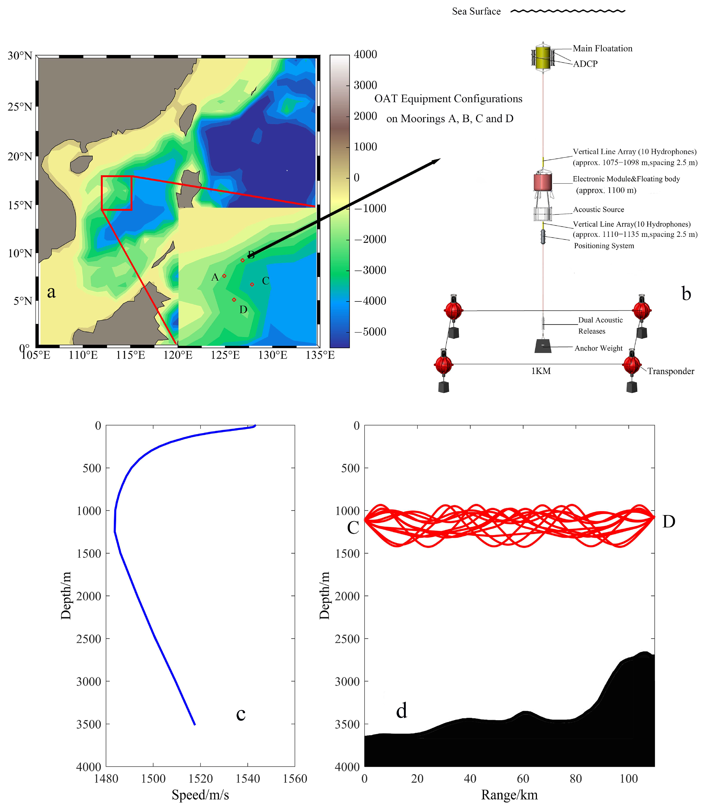
2.1. 2021 SCS OAT Experiment Data

The 2021 OAT experiment was conducted in the northern SCS from 11 July to 15 August in the area with depths ranging from 2000 m to 3700 m. Figure 1a plots the positions and depths of the four acoustic moorings deployed during the experiment, while Figure 1b illustrates the observation instruments attached to each mooring. A transmitting transducer, a positioning device, and two ten-element hydrophone vertical arrays form the core acoustic equipment on each mooring. Although the attached positions of the temperature and depth (TD) and CTD loggers are not shown in Figure 1b, a total of 16 TD loggers and 4 CTD loggers are tied to each mooring at roughly the same depth among the four moorings.

Table 1. Seawater and hydrophones depths at the four acoustic moorings.

Mooring	Water Depth/m	Location	Depth Range of Hydrophones/m	Spacing/m	Numbers of Hydrophones
A	2168	18.06°N, 113.51°E	1075–1097.5	2.5	10
			1102.5–1125	2.5	10
B	2490	18.70°N, 114.29°E	1065–1087.5	2.5	10
			1102.5–1125	2.5	10
C	3620	17.69°N, 114.71°E	1076–1098.5	2.5	10
			1113.5–1136	2.5	10
D	2700	17.05°N, 113.92°E	1076–1098.5	2.5	10
			1113.5–1136	2.5	10

shows the seawater and hydrophones depth and location at each mooring, and

Table 2. Distance between each pair of moorings.

Mooring Pair	Distance between Moorings/km
A–B	109.81
A–C	133.26
A–D	120.12
B–C	120.72
B–D	187.80
C–D	109.39

shows the distance between each pair of moorings.

The sound speed profile measured by CTD deployment in the experimental sea area shows that the sound channel axis depth is approximately 1100 m (Figure 1c). The four transmitting transducers on each mooring were placed at a depth of approximately 1100 m, and No. 1–20 hydrophones were attached to each mooring at 1075 to 1135 m depth with 2.5 m spacing for transmission/reception around the sound channel axis. Every mooring transmitted m-sequence source signal sweeping between 430–530 Hz over 40.95 s duration at a source level of 186 dB re 1 μPa @ 1 m. Source signals were emitted 8 times a day beginning at 1:00 a.m. and for each transmission repeated twice with a 5 min interval. The hydrophones and their recording module on one mooring worked and collected the other three mooring transmissions continuously during the whole experiment. The exact reception depth of the vertical hydrophone array on each mooring is listed in Table 1. To trace and record the hydrophone position on each mooring, four transponders were placed along the seabed at the corners of a square with each mooring centered and the side length of four transponders was approximately 1 km, which is long baseline, high-frequency, acoustic transponder system used to monitor the motions of each mooring and every hydrophone during the OAT experiment. The long baseline systems were used to correct the acoustic travel times for the horizontal motion of the source and the receiver due to ocean currents. The displacement corrections for every hydrophone were then estimated by spline interpolation, assuming that the mooring shape was curved. Positioning errors were calculated and estimated to be less than 3 m.

2.2. Satellite Altimeter and HYCOM Data

Satellite altimeter data and HYCOM data were utilized for comparison with the actual measured data (hydrologic and acoustic data) in the experimental area. The MSLA data provided at the official website of the Copernicus Marine Environment Monitoring Service (CMEMS) (https://marine.copernicus.eu/, accessed on 16 November 2021) are downloaded to evaluate the existence, spatiotemporal variations, and motion trajectory of a passing mesoscale eddy in this study. The data, which have a spatial resolution of 1/4° × 1/4° and a temporal resolution of 1 day, are obtained by merging data from Jason–1/2/3, Environmental Satellite (ENVISAT), GEOSat Follow-on (GFO), and other satellite altimeters. To match the time of the OAT experiment, daily delay time (DT) MSLA data from 11 July to 20 August 2021, are selected for the region bounded by 15°N to 21°N and 111°E to 118°E.

This study also makes use of data from HYCOM (downloaded website https://www.ncdc.noaa.gov/data-access/model-data/ocean-nomads, accessed on 28 November 2021), which is an operational global ocean model based on mixed coordinates. HYCOM assimilates the existing observation data available, including the horizontal flow field, sea surface temperature, and salinity data. The model data have a horizontal resolution of 1/12° × 1/12° and are divided into 40 vertical layers from 0 m to 5000 m. It is demonstrated that the HYCOM model has advantages in the simulation of mesoscale eddies in the SCS [33] and is thus preferably selected for comparisons with our OAT measurements in the study. The two adjacent layers’ data at 1000 m and 1250 m near the depth of the sound channel axis are daily moving averages for 35 days from 11 July and 15 August 2021 in this study.

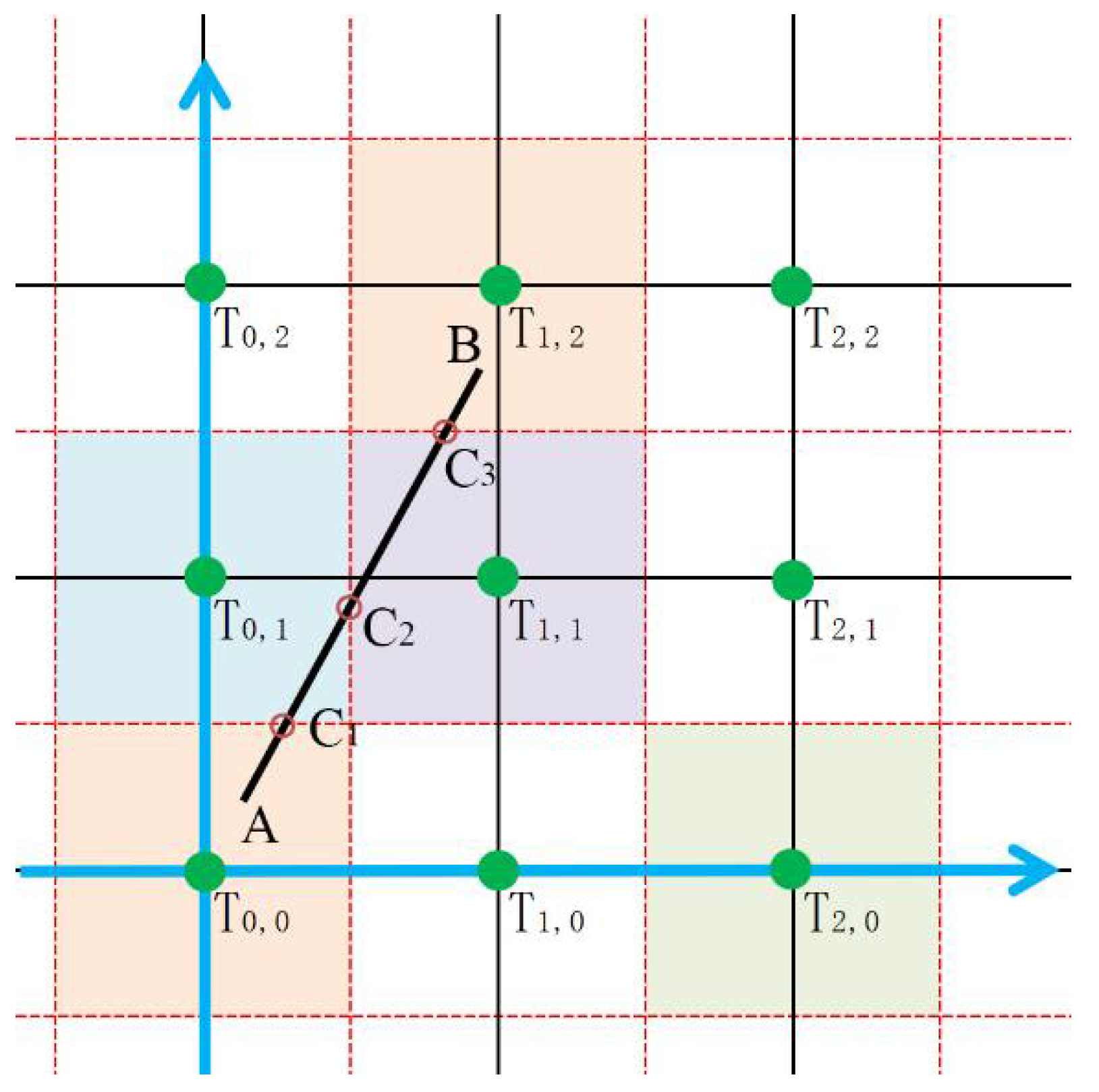
2.3. Data Processing Methods

2.3.1. Sound Speed/Temperature Conversion

Travel time is a key function of temperature, current velocity, and salinity [22]. In the absence of ocean currents, the relations between the fluctuations in temperature or salinity and associated changes in sound speed can be obtained by computing the partial derivatives of the equations for sound speed. The Mackenzie equation [35] gives

$$\frac{\partial \mathrm{C}}{\partial \mathrm{T}}=4.59-0.106\mathrm{T}+7.12\times {10}^{-4}{\mathrm{T}}^2-1.03\times {10}^{-2}\left(\mathrm{S}-35\right),$$

(1)

$$\frac{\partial \mathrm{C}}{\partial \mathrm{S}}=1.34-0.103\times {10}^{-2}\mathrm{T},$$

(2)

which describe the relative effects of temperature and salinity on sound speed. The factor relating sound speed and temperature changes is temperature dependent, as mentioned above, and weakly salinity dependent; thus, the sound speed variation induced by the pure temperature and salt variation is given with the integration over the corresponding variable (temperature or salt) interval,

$$\mathsf{\Delta }{\mathrm{C}}_{\mathrm{T}}\approx {{\displaystyle \int }}_0^{\mathsf{\Delta }\mathrm{T}}\frac{\partial \mathrm{C}}{\partial \mathrm{T}}\mathrm{dT},$$

(3)

$$\mathsf{\Delta }{\mathrm{C}}_{\mathrm{S}}\approx {{\displaystyle \int }}_0^{\mathsf{\Delta }\mathrm{S}}\frac{\partial \mathrm{C}}{\partial \mathrm{S}}\mathrm{dS},$$

(4)

At the sound channel axis of the experimental area, the temperature is approximately 4.2 °C, so temperature changes are small and can be readily derived from estimated sound speed changes using a simple scaling factor, $\mathrm{k}$, with an error of only a few percent [22],

$$\mathsf{\Delta }\mathrm{C}\approx \mathrm{kdT},$$

(5)

According to the calculation method provided by Dushaw [36], the simple scaling factor is 4.17 ms⁻¹ °C⁻¹. Thus, the estimates for sound speed can be accurately and conveniently converted to temperature estimates.

2.3.2. OAT Data Processing

Because sound rays always refract toward lower speed areas, sound waves emitted at the sound channel axis are confined and trapped near the channel considering that the sound speed is higher in the layers both above and below the sound channel axis. The eigenrays shown in Figure 1d illustrate that the majority of sound rays do not contact the sea surface or the seabed, resulting in a very small energy loss and over 100 km of sound propagation under a moderate source level. The peak arrival of the acoustic signal, which is determined after pulse compression signal processing, is used to locate the precise position of the OAT travel time series. Because the travel time depends on the hydrologically associated sound speed and the transmission and reception distance, the motion of the vertical array must be removed by a positioning device to resolve the only hydrological factor-induced sound speed variation. Nevertheless, the reciprocity law states that the acoustic pressure will remain unchanged if the source and receiver positions are interchanged. Therefore, we will not discriminate which mooring is source or receiver in the following discussion. There are two considerations for choosing the three paths AC, DC, and BA. One is the movement of the eddy from D to A, B, and C. The other is, from the MSLA and HYCOM data, the temperature at moorings B and C is more affected by the eddy than that among the rest of the four moorings. Therefore, moorings B/C are chosen as one end of the path, while moorings A/D are chosen as the other end of the path to better illustrate the OAT experimental results and to better compare the OAT data with MSLA or HYCOM data.

The sound speed, which is obtained by dividing the travel time by the distance between the moorings, is smoothed by 8 transmissions to obtain a one-day average since the temporal resolution of the HYCOM data is 1 day. Meanwhile, each mooring has a total of 16 TD and 4 CTD measurements ranging in depth from 200 m to 1550 m. The temperature data at a depth of approximately 1100 m were used herein by spline interpolation of the above depth data and have a temporal resolution of 1 min and range from 1:00 a.m. on 11 July to 1:00 a.m. on 15 August totaling 35 days. To facilitate a comparison with the corresponding HYCOM data, which are resolved in days, the recorded TD/CTD temperature measurements are smoothed to obtain the daily moving average temperature.

2.3.3. Processing of HYCOM Data

The temperature change at the sound channel axis depth (1100 m) was relatively weak relative to the pelagic depth; at the same time, the HYCOM data only had two layers of data at 1000 m and 1250 m at this depth. The HYCOM temperature at 1100 m depth is obtained by interpolation from the adjacent layers of 1000 m and 1250 m depth data. To obtain the temperature anomalies caused by the mesoscale eddy in the experimental sea area, we need the background temperature of the same experimental area. However, it is worth noting that the background field cannot be removed using 6° × 6° grid median filtering [37] because the experimental sea area is surrounded by land. Hence, the background field is obtained by temporally averaging the HYCOM data from 1 to 10 July; during the period, there is no obvious eddy from the sea level anomaly of the merged altimeter data. The temperature anomaly at a depth of 1100 m is then calculated by subtracting the matching background temperatures from the 11 July to 20 August data, yielding the temperature temporal variations at a depth of 1100 m at the four moorings.

Then, we need a path-averaged algorithm to compute the average temperature along the sound propagation path at the four moorings. The average temperature on each path is calculated using a length-weighted averaging algorithm, which is based on differential techniques. Suppose Figure 2 is a plane grid that represents the interpolated layer of HYCOM data at the sound channel axis depth. The green dots represent the HYCOM grid data, marked ${\mathrm{T}}_{\mathrm{i},\mathrm{j}}$ (The footmarkers i, j stand for the transversal and longitudinal points of the lattice respectively). A and B represent the two points of transmitter and receiver location, respectively. Assume that the temperature data of each grid point represent the temperature of all “points” within a certain surrounding area. The temperature values within the range of 1/2 grid length on the left and right sides and 1/2 grid width on the upper and lower sides of a grid point can be regarded as equal to that of the grid point. For example, assume that the temperature of ${\mathrm{T}}_{2,0}$ is V; then, the temperature value of all “points” in the surrounding green box is V. Next, the direct propagation path with endpoints A and B is divided into several line segments, as shown in Figure 2. The temperature of each line segment depends on which square it falls into, and the temperature of the segment equals that of the grid-centered square. Meanwhile, the length proportion of each line segment relative to the total path length can also be computed. In this way, the average temperature on the direct path AB can be obtained by summing the length-weighted temperatures of all segments together, which multiplies the temperature of each line segment by the proportion of the line segment in the path,

$${\overline{\mathrm{T}}}_{\mathrm{A}\mathrm{B}}={\mathrm{T}}_{0,0}·\frac{\mathrm{A}{\mathrm{C}}_1}{\mathrm{A}\mathrm{B}}+{\mathrm{T}}_{0,1}·\frac{{\mathrm{C}}_1{\mathrm{C}}_2}{\mathrm{AB}}+{\mathrm{T}}_{1,1}·\frac{{\mathrm{C}}_2{\mathrm{C}}_3}{\mathrm{AB}}+{\mathrm{T}}_{1,2}·\frac{{\mathrm{C}}_3\mathrm{B}}{\mathrm{AB}}$$

(6)

where ${\overline{\mathrm{T}}}_{\mathrm{AB}}$ stands for the average temperature on path A–B, ${\mathrm{T}}_{\mathrm{i},\mathrm{j}}$ is the grid temperature data in the HYCOM data, in which the footmarkers i, j stand for the transversal and longitudinal points of the lattice respectively and ${\mathrm{AC}}_1/{\mathrm{C}}_1{\mathrm{C}}_2/{\mathrm{C}}_2{\mathrm{C}}_3/{\mathrm{C}}_3\mathrm{B}/\mathrm{AB}$ is the line segment length between two points in Figure 2.

Finally, the path-averaged temperature time series of the eddy in the HYCOM data are compared with those estimated from the sound speed variation of the OAT.

3. Movement of the Eddy from Altimeters and HYCOM Data

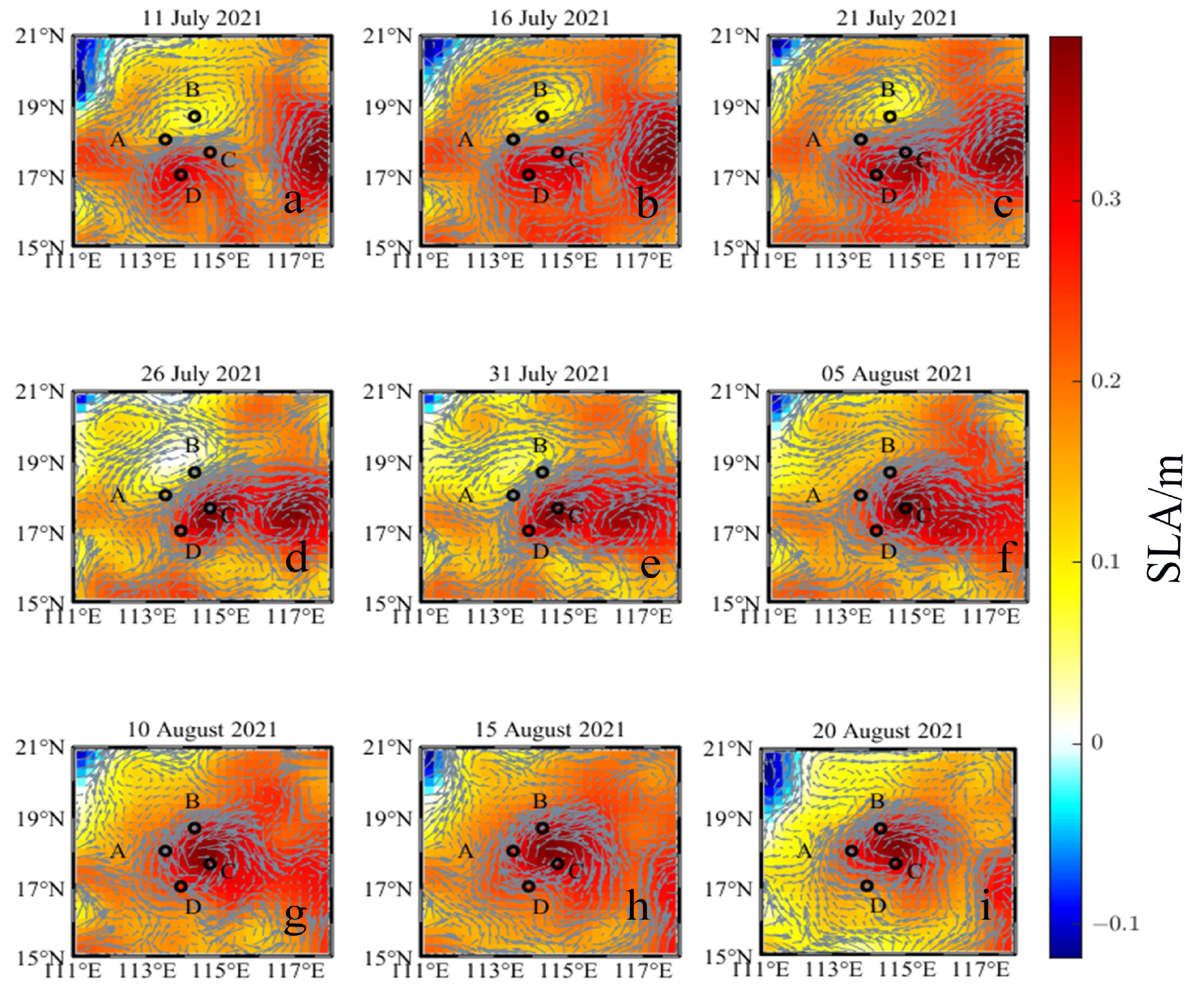
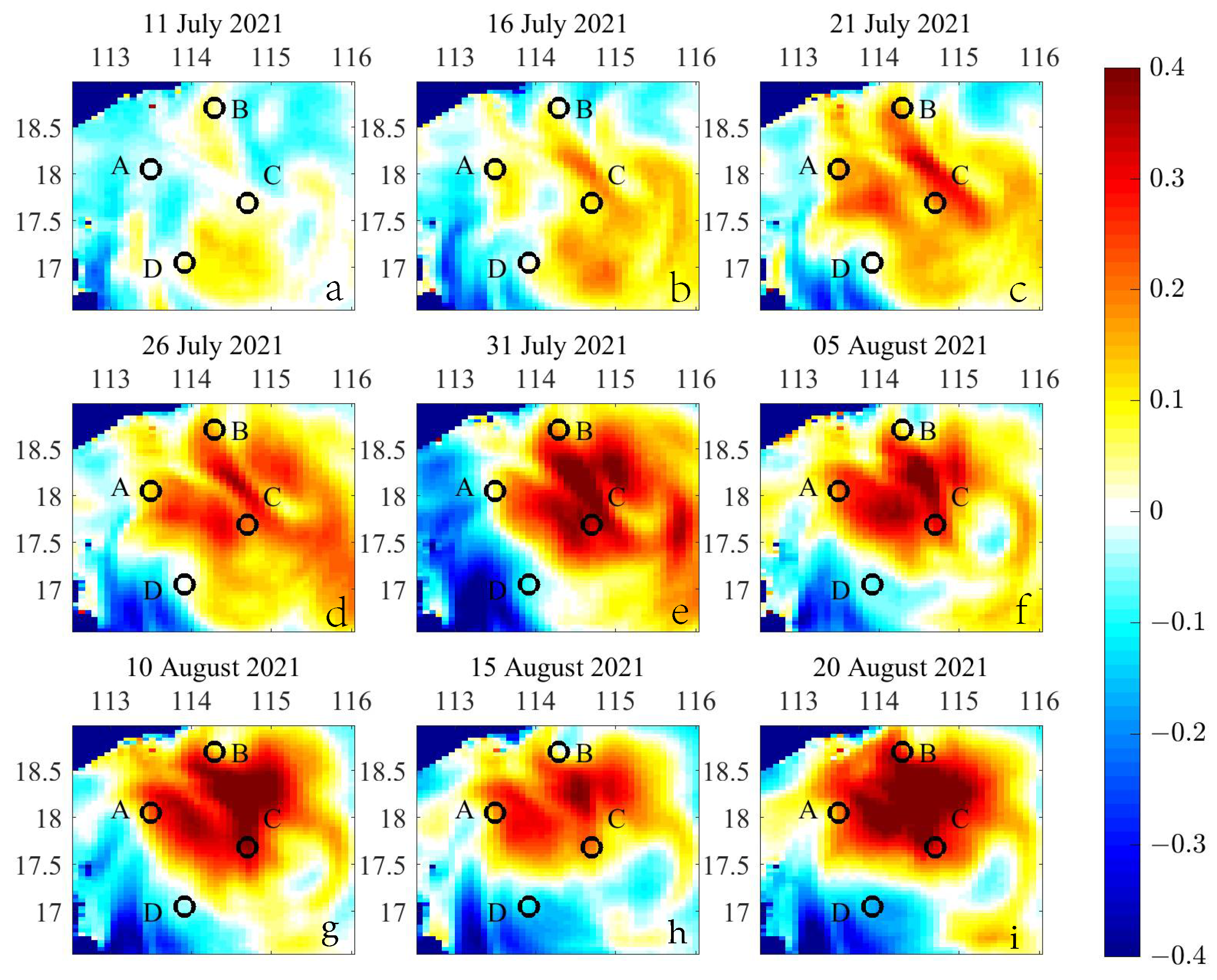
3.1. The Movement of the Eddy Imaged by Altimeters

As shown in Figure 3a, a pair of mesoscale warm eddies (a cascade of two warm eddies) formed in the early stages of the OAT experiment beginning on 11 July 2021. The two eddies merged together into a single eddy before 31 July and migrated during the development phase. The merged mesoscale eddy progressively strengthened in the experimental sea area; moreover, the eddy profile gradually became clearer. In the beginning, the eddy affected only moorings C and D, but as the eddy moved, it influenced all four moorings to varying degrees. Mooring A was always at the edge of the eddy, and mooring C was always encompassed by the warm eddy; moreover, the edge of the warm eddy moved away from mooring D gradually, and the eddy gradually moved toward mooring B. In brief, the warm eddy gradually moved northward and slightly eastward.

3.2. The Warm Eddy Captured by HYCOM Data

The temperature anomaly associated with the eddy center in summer is believed to be centrosymmetric across the whole water column according to a composite analysis of the eddy center [38]; therefore, it is feasible to utilize the temperature anomaly in the HYCOM data to represent the movement of the eddy. The eddy influence depth is clearly shown on the temperature anomaly profile (Figure 4) after the HYCOM data are daily moving averaged while the moorings work. Because the eddy temperature anomaly exceeded depths of 1400 m, it directly affected the water body along the sound channel axis, as illustrated in Figure 4. Figure 5a–i presents the eddy in the HYCOM data at a depth of 50 m for comparison with the MSLA data. The strength of the warm eddy steadily increased over time as it moved northeast. The eddy was close to mooring D at first, barely impacting mooring C. As it developed and moved, however, it affected moorings A, B, and C while traveling away from mooring D, and by 31 July, it did not influence mooring D at all.

Figure 6 displays the temperature variations of the four moorings at depth of 1100 m in the HYCOM data and “virtual” (see below for the meaning of “virtual”) TD/CTD measurements. For the HYCOM data, the daily temperature of the moorings at 1100 m is obtained by interpolation of the four nearest grid data, whereas the temperature of “virtual” TD/CTD (hereafter referred to hereafter as TD/CTD-measured temperature in brief) at 1100 m depth is also obtained by spline interpolation of a total of 16 TD and 4 CTD measurements ranging in depth from 200 m to 1550 m. The mooring A temperature in HYCOM at a depth of 1100 m progressively rose over time due to the development and approaching of the warm eddy. In contrast, the mooring B temperature in HYCOM at depth of 1100 m increased and then declined over the 35-day period, although it remained relatively steady. This is because the warm eddy had no impact on mooring B at the start; when its edge approached mooring B later, its temperature was slightly changed. The mooring C temperature in HYCOM increased with time, possessing the highest climbing rate among the four moorings also because mooring C was most in close proximity to the eddy center, whereas mooring D temperature steadily dropped over time, resulting from the warm eddy moving progressively farther away.

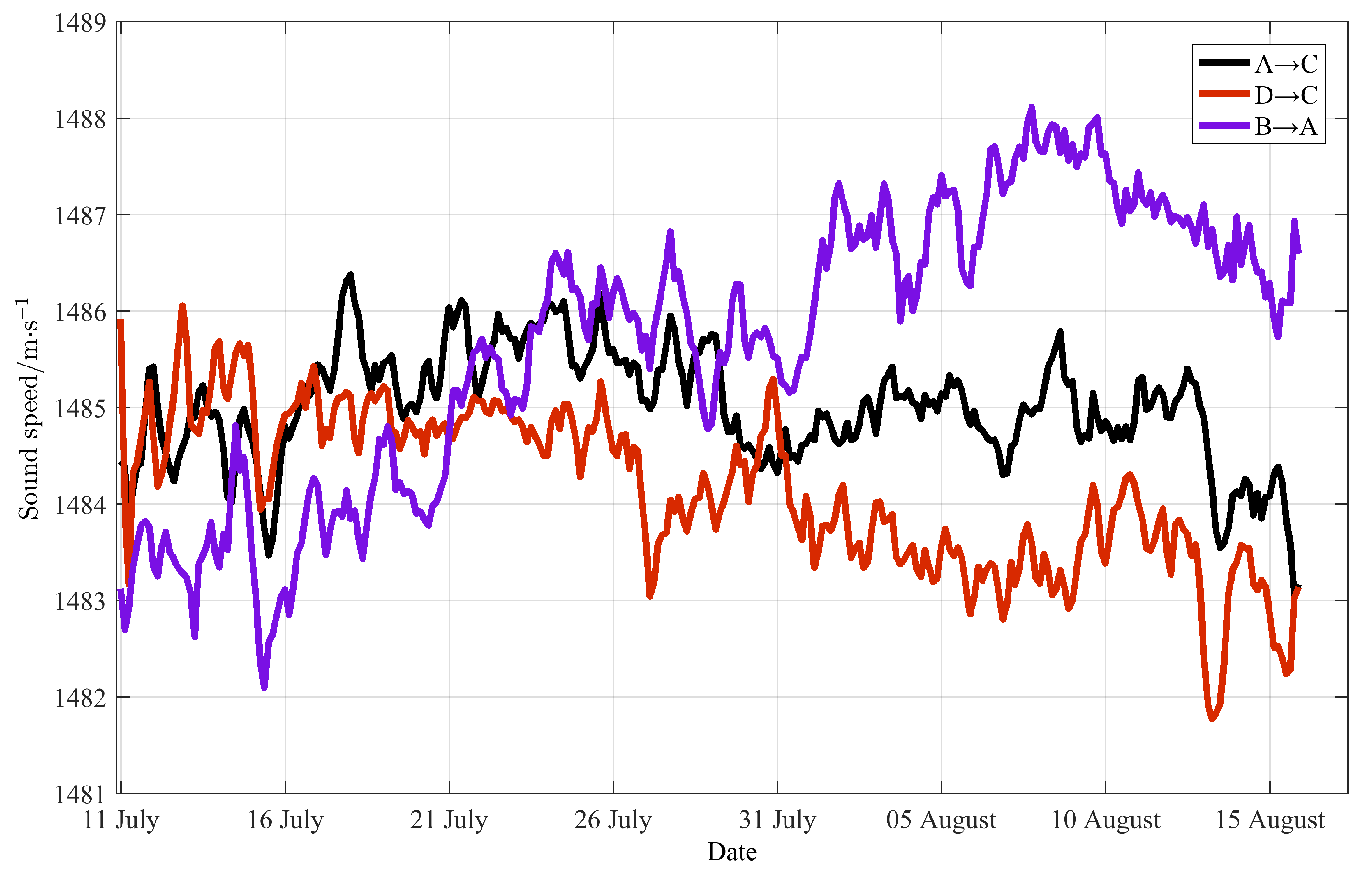
4. Results of the OAT Experiment

OAT was originally conceived as integral observations of the ocean and a way to estimate path-averaged sound speed over range. Acoustic rays provide a natural measure of this quantity [22]. Within the inverse scheme, one could certainly compute a path-averaged sound speed along a single eigenray as a function of range; however, the uncertainties associated with such a scheme would be so large as to make such computation less meaningful. On the other hand, it is important to recognize that since all eigenrays arrive at approximately the same time, it does not matter which ray was assigned to which arrival peak, at least to the first order [29]. For this reason, it is not obligatory to resolve every eigenray and compute each arrival time along a single eigenray. Instead, it is often preferred to compute the range-average of the sound speed of all eigenrays, which has small uncertainty. It is well known that an oceanographically meaningful quantity is the average. To obtain an estimate of temperature, therefore, the appropriate average sound speed quantity is calculated in this paper, and this quantity and its uncertainty were scaled to obtain temperature [36]. The fluctuation of the daily averaged travel time of the acoustic signal can be used to characterize the temperature properties of water near the sound channel axis and for comparison with those in the HYCOM data.

In this experiment, 20 hydrophones were attached to the mooring line vertically at depths near the sound channel axis. Figure 7a–c shows that the variation in sound velocity with time obtained from the array received by the 20 hydrophones is very consistent whether they are received from station C and transmitted from station A (Figure 7a)/D (Figure 7b) or received from station A and transmitted from station B (Figure 7c). To demonstrate this consistency, the correlation coefficients are calculated between different hydrophones, except for the malfunction of the No. 5, 14, and 19 hydrophones, the correlation coefficients of the time series are more than 0.97. Therefore, we only need to choose the time series of one hydrophone for analysis (hereinafter the second hydrophone).

The increase in the daily average travel times of the signals between moorings D and C indicates that sound speed dropped dramatically over time between D and C from 1486 m/s to 1482 m/s. Such a reduction in the sound speed implies a temperature drop, which further shows that the average temperature on path D–C declined over time (shown in Figure 8), with the maximum sound speed difference reaching 4 m/s, while signals transmitted by mooring A and received by mooring C yielded relatively constant sound speed estimation throughout time, meaning that the A–C path-averaged temperature variation is 1485 ± 1 m/s, which is nearly negligible. The propagation speed of sound transmitted by mooring B and received by mooring A increased significantly over time from 1482 m/s to 1488 m/s with a maximum difference of 6 m/s, which also means an increase in temperature. The variation in the sound speed along the sound channel axis indicates that hydrological factors, notably water temperature, varied due to the eddy motion.

Additionally, the TD/CTD-measured temperatures at mooring A at depth of 1100 m increased somewhat over time. The TD/CTD-measured temperatures at mooring B increased the most, while those at mooring C were practically stable and typically constant. In contrast, the temperatures measured at mooring D slowly fell (see Figure 6, solid curves).

5. Comparison of the Eddy Using Multisource Data

5.1. Comparison of the Eddy Movement between the MSLA and HYCOM Data

As shown in Figure 3a, the warm eddy imaged by MSLA began to affect moorings C and D on 11 July, with mooring C being influenced by the warm eddy center and mooring A being touched by its edge. The eddy progressively influenced mooring B while drifting northeastward and eventually severely impacted mooring B after 31 July. Although the temperature anomaly of the warm eddy in HYCOM (Figure 5a–i) only marginally affected mooring D at a depth of 50 m, it had almost no manifestation on mooring C from 11 July. Beginning approximately on 21 July, according to the HYCOM data, the eddy began to affect moorings A, B, and C as the eddy intensified and moved northeast. By 31 July, the eddy had completely stopped impacting mooring D. In brief the HYCOM data indicate that the eddy had the most visible influence on mooring C, whereas the eddy recorded by satellite altimeters had the most obvious influence on mooring B. Consequently, the movement of the mesoscale eddy in the HYCOM data is not entirely compatible with those observed by the satellite altimeters.

5.2. Comparison of Temperature between MSLA and TD/CTD

Comparing Figure 6 and Figure 9a–i reveals that the TD/CTD-measured temperature at mooring A slightly increased as a result of being near the edge of the eddy (also seen in the sea surface height anomaly maps). According to the sea surface height anomaly maps, the largest recorded temperature rise at mooring B occurred due to a temperature shift from being unaffected to being gradually influenced by the warm eddy. The TD/CTD-measured temperature at mooring C remained essentially constant, indicating that mooring C temperature was constant inside the warm eddy, which was confirmed by the sea surface height anomaly maps. Finally, the progressive drop in the temperatures recorded at mooring D is attributed to the gradual departure of the warm eddy from mooring D. These findings support that the TD/CTD-measured temperature fluctuations at each mooring match the sea surface height anomalies well.

5.3. Comparison of Temperature between TD/CTD and HYCOM

However, the eddy at depth of 1100 m at every mooring location in the HYCOM data tells a different story from that of the TD/CTD-measured temperatures. Figure 6 shows that the temporal temperature variations in HYCOM at moorings A and D (solid curve) are both similar to those measured by the TD/CTD loggers. The HYCOM temperature at mooring B remained generally stable over time, while the TD/CTD-measured temperature increased considerably from 3.56 to 4.12 °C. Conversely, the HYCOM temperature at mooring C increased during the experiment (from 3.67 to 3.91 °C), while the TD/CTD-measured temperature fluctuated between 4.1 and 4.2 °C. The fact that the temperature changes at moorings B and C in HYCOM are quite different from the TD/CTD-measured data demonstrates that the experimental starting position and movement of the eddy in the HYCOM data differ significantly from those indicated by the satellite altimeters and the TD/CTD in situ measurements, suggesting the deficiencies of the HYCOM model. Furthermore, the temperature fluctuations (from 3.54 °C to 4.25 °C, see orange cross-marks on two dashed curves), among the four moorings are greater than those in the HYCOM data (from 3.58 °C to 3.90 °C see orange cross-marks on two solid curves), implying that the modeled eddy intensity is at least two times less than the measured eddy intensity. This finding is consistent with Sagen [29], who claims that comparable model variations are much weaker, indicating that the model underestimates the intensity of the mesoscale.

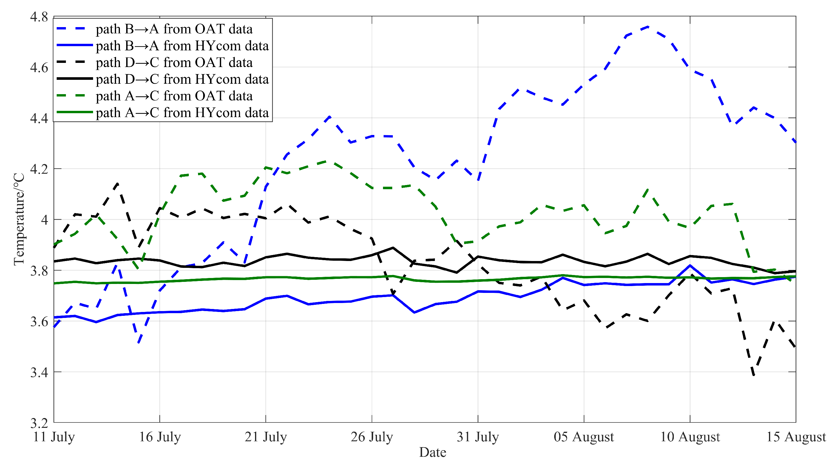
5.4. Comparison of the Eddy Temperature between the OAT and HYCOM Data

5.4.1. Comparison of the Eddy Movement at the Sound Channel Axis Depth

As mentioned above, a comparison of the eddy movement between the OAT and HYCOM temperatures is made at the depth of the sound channel axis. The acoustic data can be used to obtain estimates of sound speed variations and then temperature variations by the use of sound speed to temperature conversion. The average temperature on path D–C declined by 1.04 °C, with the temperature at mooring C remaining essentially constant and that at mooring D dropping (Figure 6). The temperature reduction on path D–C within the deep sound channel is consistent with the warm eddy movement recorded by satellite altimeters (Figure 3a–i), which demonstrates that the eddy gradually departed from mooring D during this period. The sound speed increase on path B–A (Figure 8) indicates that the average temperature on the path rose 1.40 °C. Furthermore, the largest increase in sound speed coincides with the maximal rise in the OAT-derived average temperature, which is compatible with the satellite altimeter observation that mooring B went from being unaffected to being influenced by the warm eddy while mooring A remained at the eddy edge. The sound propagation path B–A (not the path D–C) displays the greatest perturbation in sound speed, indicating that the temperature at mooring B changed the most, whereas the HYCOM data indicate the greatest temperature change occurred at mooring C, revealing that the HYCOM data are not precise enough at 1100 m depth. The presence of the eddy between mooring A and mooring C resulted in a sound speed fluctuation between 1483.5 and 1486 m/s; thus, the temperature variations (maximum not exceeding 0.75 °C) on path A–C were not noticeable during the experiment. Ultimately, the eddy path-averaged temperatures at the depth of the sound channel axis recorded by OAT are compatible with those imaged by satellite altimeters but are distinct from those described by the HYCOM data.

5.4.2. Difference in the Eddy Temperature at the Sound Channel Axis Depth between OAT and HYCOM

The sound speed at the started/ended experiment date (11 July/15 August) is not excluded in the following comparison because we cannot find enough eight transmission/reception data points to perform the moving average. The sound speed on the B–A path at the sound channel axis depth was the lowest (1482.1 m/s) on 15 July and the highest (1488.2 m/s) on 8 August, as shown in Figure 8. The maximum difference is 6 m/s. Because the sound speed on path B–A reflects the average temperature effect on the sound propagation path, it is necessary to obtain the average temperature change on this path in HYCOM for comparison (Figure 6). The temperature change on path B–A calculated from the HYCOM data is 0.13 °C. Similarly, the sound speed on path D–C was the largest (1486.1 m/s) on 13 July and the smallest (1481.8 m/s) on 14 August. The maximum difference is 4 m/s. Correspondingly, the temperature variation in the HYCOM data changed by 0.19 °C. In the HYCOM data, the temperature variation on path D–C was greater than that on path B–A, indicating that the eddy represented by the HYCOM data exerted a stronger influence on mooring C than on mooring B. At the depth of the sound channel axis (the temperature is typically in the range of 4 °C), for every 1 °C change in temperature, the corresponding change in sound speed is 4.17 m/s. According to the OAT results, the measured sound speed on path B–A changed by as much as 6 m/s, so the corresponding temperature change was within 1.44 °C. The measured sound speed variation on path D–C was 4 m/s; the corresponding temperature change was less than 0.96 °C. We can conclude that the measured temperatures derived from the sound speed are significantly (at least five times) greater than the HYCOM data, which demonstrates that the HYCOM data are not precise enough to capture the temperature anomaly of the warm eddy, at least not precise at the depth of the sound channel axis (1100 m) in this study. The temperature change difference between the OAT and HYCOM data is shown in Figure 10. The maximum sound velocity difference and temperature difference obtained by each hydrophone are listed in

Table 3. Maximum sound speed and temperature variation for the 20 hydrophones.

		D→C		B→A		A→C
	Difference	Sound Speed/ms−1	Temperature/°C	Sound Speed	Temperature	Sound Speed	Temperature
Hydrophone
No. 1		4.23	1.02	6.02	1.44	3.20	0.77
No. 2		4.28	1.03	6.02	1.44	3.33	0.80
No. 3		4.28	1.03	5.93	1.42	3.18	0.76
No. 4		4.25	1.02	5.94	1.43	3.15	0.75
No. 5		-	-	6.03	1.44	-	-
No. 6		4.24	1.02	5.93	1.42	3.06	0.74
No. 7		4.25	1.02	6.01	1.44	3.13	0.75
No. 8		4.28	1.03	6.02	1.44	3.13	0.75
No. 9		4.23	1.01	6.24	1.50	3.15	0.76
No. 10		4.20	1.01	6.00	1.44	3.16	0.76
No. 11		4.50	1.08	6.18	1.48	3.21	0.77
No. 12		4.48	1.07	6.40	1.53	3.19	0.77
No. 13		4.47	1.07	5.96	1.43	3.16	0.756
No. 14		-	-	6.05	1.45	-	-
No. 15		4.47	1.07	6.09	1.46	3.12	0.75
No. 16		4.45	1.07	6.07	1.46	3.02	0.72
No. 17		4.37	1.05	4.37	1.05	3.03	0.73
No. 18		4.37	1.05	4.37	1.05	3.04	0.73
No. 19		-	-	6.87	1.65	-	-
No. 20		4.40	1.05	4.40	1.05	2.98	0.72
Mean Value		4.34	1.04	5.85	1.40	3.13	0.75
HYCOM Result		NA	0.19	NA	0.13	NA	0.04

showing that the OAT temperature variation averaged over 20 hydrophones is at least 5 times that of the HYCOM-derived temperature data. The OAT experimental data-derived temperature variations are much greater than those in the HYCOM model.

6. Discussion

The above result is reasonable by comparison with H. Sagen’s work, in which a regional high-resolution Fram Strait Model based on HYCOM was shown to greatly underestimate the intensity of mesoscale fluctuations and to exhibit a warm bias of approximately 0.38 °C in path-averaged temperature, although rich observation data in the upper layer were assimilated in the above model [37]. It is not surprising that the HYCOM model used in this article, which is not specifically targeted and tuned at the experimental area and not much field data at the sound channel axis are assimilated in the HYCOM model, produces results that are five times smaller than the observed OAT measurements. The discovery is valuable for temperature-related eddy research, particularly for eddy studies at the sound channel axis. To put it another way, limited by the data provided by the OAT experiment (e.g., the hydrophone does not have full depth coverage and lacks flow data), only the eddy temperature at the depth of the sound channel axis was investigated in this paper, and further research is needed to detect temperature changes at other depths or even three-dimensional structures of the eddy by OAT. Nevertheless, an OAT method for detecting the movement and temperature evolution of a mesoscale eddy is demonstrated in this article. OAT provides a data type that is both accurate and complementary to data from other moored/point observations. On the other hand, OAT can improve high-resolution ocean models through data assimilation techniques; the use of acoustic travel times as constraints on the ocean model, through data assimilation or other means, could be expected to correct some of the model deficiencies, particularly at deep layers such as sound channel axis depth where there is not rich observation data in comparison with the above mixed layer. OAT measurements also have the advantage of providing long time series data at a specific space which is very efficient in model output improvement.

7. Conclusions

For a comparative study of the temperature change in a warm eddy, the existence of a mesoscale eddy is first confirmed both by satellite altimeter and HYCOM model data in the experimental sea area. The temperature changes measured by TD/CTD and by the OAT sound speed (temperature estimates were readily obtained from the sound speed estimates) are in accordance with those captured on the MSLA image during the evolution of the eddy. This article demonstrates the possibility that OAT can be leveraged to quantify the temperature change and even the movement of a mesoscale eddy in deep waters. However, the eddy temperature changes prompted by the HYCOM data is at least two times less than that measured by TD/CTD. Moreover, the transmission/reception path-averaged temperature change in the eddy in the HYCOM data is inconsistent with that derived from the sound speed of the acoustic signal recorded by the OAT, including both inconsistencies in the eddy temperature evolution and movement. Furthermore, the OAT temperature changes at the depth of the sound channel axis are five times greater than those path-averaged in the HYCOM data. These findings demonstrate that OAT is also feasible as a tool to study the properties of mesoscale eddies at depth. At the same time, the HYCOM data are insufficiently accurate, at least at the depth of the sound channel axis in this investigation, which means OAT can improve high-resolution ocean models through data assimilation.

References

1. Cai, S.; Xie, J.; He, J. An Overview of Internal Solitary Waves in the South China Sea. Surv. Geophys. 2012, 33, 927–943. [Google Scholar] [CrossRef]
2. Hong, D.-B.; Yang, C.-S.; Ouchi, K. Estimation of Internal Wave Velocity in the Shallow South China Sea Using Single and Multiple Satellite Images. Remote Sens. Lett. 2015, 6, 448–457. [Google Scholar] [CrossRef]
3. Chu, P.C.; Fan, C.; Lozano, C.J.; Kerling, J.L. An Airborne Expendable Bathythermograph Survey of the South China Sea, May 1995. J. Geophys. Res. Oceans 1998, 103, 21637–21652. [Google Scholar] [CrossRef]
4. Xiu, P.; Chai, F.; Shi, L.; Xue, H.; Chao, Y. A Census of Eddy Activities in the South China Sea during 1993–2007. J. Geophys. Res. 2010, 115, C03012. [Google Scholar] [CrossRef] [Green Version]
5. Lin, X.; Dong, C.; Chen, D.; Liu, Y.; Yang, J.; Zou, B.; Guan, Y. Three-Dimensional Properties of Mesoscale Eddies in the South China Sea Based on Eddy-Resolving Model Output. Deep Sea Res. Part Oceanogr. Res. Pap. 2015, 99, 46–64. [Google Scholar] [CrossRef]
6. Klein, P.; Lapeyre, G.; Siegelman, L.; Qiu, B.; Fu, L.-L.; Torres, H.; Su, Z.; Menemenlis, D.; Gentil, S.L. Ocean-Scale Interactions from Space. Earth Space Sci. 2019, 6, 795–817. [Google Scholar] [CrossRef] [Green Version]
7. Ferrari, R.; Wunsch, C. Ocean Circulation Kinetic Energy: Reservoirs, Sources, and Sinks. Annu. Rev. Fluid Mech. 2008, 4, 253–282. [Google Scholar] [CrossRef] [Green Version]
8. Wolfe, C.L.; Cessi, P.; McClean, J.L.; Maltrud, M.E. Vertical Heat Transport in Eddying Ocean Models. Geophys. Res. Lett. 2008, 35. [Google Scholar] [CrossRef] [Green Version]
9. McGillicuddy, D.J. Mechanisms of Physical-Biological-Biogeochemical Interaction at the Oceanic Mesoscale. Annu. Rev. Mar. Sci. 2016, 8, 125–159. [Google Scholar] [CrossRef] [Green Version]
10. Vastano, A.C.; Owens, G.E. On the Acoustic Characteristics of a Gulf Stream Cyclonic Ring. J. Phys. Oceanogr. 1973, 3, 470–478. [Google Scholar] [CrossRef]
11. Weinberg, N.L.; Zabalgogeazcoa, X. Coherent Ray Propagation through a Gulf Stream Ring. J. Acoust. Soc. Am. 1977, 62, 888. [Google Scholar] [CrossRef]
12. Mikryukov, A.V.; Popov, O.E. Penetration of Sound into the Cold Eddy of the Sargasso Sea. Acoust. Phys. 2008, 54, 77–83. [Google Scholar] [CrossRef]
13. Zhang, Z.; Wang, W.; Qiu, B. Oceanic Mass Transport by Mesoscale Eddies. Science 2014, 345, 322–324. [Google Scholar] [CrossRef] [PubMed]
14. Shang, E.C.; Wang, Y.Y. ACOUSTIC TRAVEL TIME COMPUTATION BASED ON PE SOLUTION. J. Comput. Acoust. 1993, 1, 91–100. [Google Scholar] [CrossRef]
15. Baer, R.N. Calculations of Sound Propagation through an Eddy. J. Acoust. Soc. Am. 1980, 67, 1180–1185. [Google Scholar] [CrossRef]
16. Jian, Y.J.; Zhang, J.; Liu, Q.S.; Wang, Y.F. Effect of Mesoscale Eddies on Underwater Sound Propagation. Appl. Acoust. 2009, 70, 432–440. [Google Scholar] [CrossRef]
17. Munk, W.H. Horizontal Deflection of Acoustic Paths by Mesoscale Eddies. J. Phys. Oceanogr. 1980, 10, 596–604. [Google Scholar] [CrossRef]
18. Weinberg, N.L.; Clark, J.G. Horizontal Acoustic Refraction through Ocean Mesoscale Eddies and Fronts. J. Acoust. Soc. Am. 1980, 68, 703–705. [Google Scholar] [CrossRef]
19. Mellberg, L.E.; Robinson, A.R.; Botseas, G. Azimuthal Variation of Low-Frequency Acoustic Propagation through Asymmetric Gulf Stream Eddies. J. Acoust. Soc. Am. 1991, 89, 2157–2167. [Google Scholar] [CrossRef]
20. Lawrence, M.W. Modeling of Acoustic Propagation across Warm-core Eddies. J. Acoust. Soc. Am. 1983, 73, 474–485. [Google Scholar] [CrossRef]
21. Munk, W.; Wunsch, C. Ocean Acoustic Tomography: A Scheme for Large Scale Monitoring. Deep Sea Res. Part Oceanogr. Res. Pap. 1979, 26, 123–161. [Google Scholar] [CrossRef]
22. Munk, W.; Worcester, P.; Wunsch, C. Ocean Acoustic Tomography; Cambridge University Press: Cambridge, UK, 1995. [Google Scholar]
23. Elisseeff, P.; Schmidt, H.; Wen, X. Ocean Acoustic Tomography as a Data Assimilation Problem. IEEE J. Ocean. Eng. 2002, 27, 275–282. [Google Scholar] [CrossRef]
24. Skarsoulis, E.K.; Cornuelle, B.D. Travel-Time Sensitivity Kernels in Ocean Acoustic Tomography. J. Acoust. Soc. Am. 2004, 116, 227–238. [Google Scholar] [CrossRef]
25. Duda, T.F.; Flatté, S.M.; Colosi, J.A.; Cornuelle, B.D.; Hildebrand, J.A.; Hodgkiss, W.S.; Worcester, P.F.; Howe, B.M.; Mercer, J.A.; Spindel, R.C. Measured Wave-front Fluctuations in 1000-km Pulse Propagation in the Pacific Ocean. J. Acoust. Soc. Am. 1992, 92, 939–955. [Google Scholar] [CrossRef]
26. Skarsoulis, E.K.; Athanassoulis, G.A.; Send, U. Ocean Acoustic Tomography Based on Peak Arrivals. J. Acoust. Soc. Am. 1996, 100, 797–813. [Google Scholar] [CrossRef]
27. Colosi, J.A.; Van Uffelen, L.J.; Cornuelle, B.D.; Dzieciuch, M.A.; Worcester, P.F.; Dushaw, B.D.; Ramp, S.R. Observations of Sound-Speed Fluctuations in the Western Philippine Sea in the Spring of 2009. J. Acoust. Soc. Am. 2013, 134, 3185–3200. [Google Scholar] [CrossRef] [PubMed] [Green Version]
28. Worcester, P.F.; Dzieciuch, M.A.; Mercer, J.A.; Andrew, R.K.; Dushaw, B.D.; Baggeroer, A.B.; Heaney, K.D.; D’Spain, G.L.; Colosi, J.A.; Stephen, R.A.; et al. The North Pacific Acoustic Laboratory Deep-Water Acoustic Propagation Experiments in the Philippine Sea. J. Acoust. Soc. Am. 2013, 134, 3359–3375. [Google Scholar] [CrossRef] [Green Version]
29. Sagen, H.; Dushaw, B.D.; Skarsoulis, E.K.; Dumont, D.; Dzieciuch, M.A.; Beszczynska-Möller, A. Time Series of Temperature in Fram Strait Determined from the 2008–2009 DAMOCLES Acoustic Tomography Measurements and an Ocean Model. J. Geophys. Res. Oceans 2016, 121, 4601–4617. [Google Scholar] [CrossRef]
30. Liu, J.; Piao, S.; Gong, L.; Zhang, M.; Guo, Y.; Zhang, S. The Effect of Mesoscale Eddy on the Characteristic of Sound Propagation. J. Mar. Sci. Eng. 2021, 9, 787. [Google Scholar] [CrossRef]
31. Ji, X.; Zhao, H. Three-Dimensional Sound Speed Inversion in South China Sea Using Ocean Acoustic Tomography Combined with Pressure Inverted Echo Sounders. In Proceedings of the Global Oceans 2020: Singapore-U.S. Gulf Coast, Biloxi, MS, USA, 5 October 2020; IEEE: Piscataway, NJ, USA, 2020; pp. 1–6. [Google Scholar]
32. Ji, X.; Cheng, L.; Zhao, H. Physics-Guided Reduced-Order Representation of Three-Dimensional Sound Speed Fields with Ocean Mesoscale Eddies. Remote Sens. 2022, 14, 5860. [Google Scholar] [CrossRef]
33. Worcester, P.F.; Cornuelle, B.D.; Dzieciuch, M.A.; Munk, W.H.; Howe, B.M.; Mercer, J.A.; Spindel, R.C.; Colosi, J.A.; Metzger, K.; Birdsall, T.G.; et al. A Test of Basin-Scale Acoustic Thermometry Using a Large-Aperture Vertical Array at 3250-Km Range in the Eastern North Pacific Ocean. J. Acoust. Soc. Am. 1999, 105, 3185–3201. [Google Scholar] [CrossRef] [Green Version]
34. Wu, L. Ocean Models Adaptability Comparison and Improvement in the South China Sea. Master’s Thesis, Wuhan University of Technology, Wuhan, China, 2013. [Google Scholar]
35. Mackenzie, K.V. Nine-term Equation for Sound Speed in the Oceans. J. Acoust. Soc. Am. 1981, 70, 807–812. [Google Scholar] [CrossRef]
36. Dushaw, B.D.; Sagen, H.; Beszczynska-Möller, A. Sound Speed as a Proxy Variable to Temperature in Fram Strait. J. Acoust. Soc. Am. 2016, 140, 622–630. [Google Scholar] [CrossRef] [PubMed] [Green Version]
37. Gaube, P.; McGillicuddy, D.J.; Chelton, D.B.; Behrenfeld, M.J.; Strutton, P.G. Regional Variations in the Influence of Mesoscale Eddies on Near-Surface Chlorophyll. J. Geophys. Res. Oceans 2014, 119, 8195–8220. [Google Scholar] [CrossRef] [Green Version]
38. Zu, Y.; Sun, S.; Zhao, W.; Li, P.; Liu, B.; Fang, Y.; Samah, A.A. Seasonal Characteristics and Formation Mechanism of the Thermohaline Structure of Mesoscale Eddy in the South China Sea. Acta Oceanol. Sin. 2019, 38, 29–38. [Google Scholar] [CrossRef]
Figure 1. Locations of the four acoustic moorings (a); configuration of an acoustic mooring (b); typical sound speed profile in the experimental sea area (c); a set of eigenrays obtained from a snapshot of the sound speed (d). The acoustic source is located at 1110 m depth approximately at the left of the figure (mooring C), and the receiver is at 1080 m depth approximately at the right (No. 2 hydrophone on mooring D).
Remotesensing 15 01650 g001
Figure 2. Schematic diagram of path-averaged temperature computation in a plane grid. The plane grid is supposed to be the layer of HYCOM data at sound channel axis depth. The green dots represent the HYCOM grid data, marked T i , j . A and B represent the two points of transmitter and receiver, respectively. Since line AC1 falls into the orange box with the central grid point T 0 , 0 , the temperature value of line AC1 is assigned as T 0 , 0 .
Remotesensing 15 01650 g002
Figure 3. Map of sea surface height anomalies in the OAT experimental sea area on the 11 July 2021 (a), 16 July 2021 (b), 21 July 2021 (c), 26 July 2021 (d), 31 July 2021 (e), 05 August 2021 (f), 10 August 2021 (g), 15 August 2021 (h), 20 August 2021 (i), and the gray arrows represent the flow velocity field. The date of the eddy evolution is shown above the center of each panel. The dots denote the locations of moorings A, B, C, and D, respectively. The specific latitude and longitude coordinates can be found in Table 1. A pair of mesoscale warm eddies formed in the early stages of the OAT experiment with the two eddies merged together into a single eddy and migrated northward and slightly eastward during the experiment.
Remotesensing 15 01650 g003
Figure 4. Temperature anomaly map of the zonal profile during the experiment. The depth profile created along 18.32°N (near the eddy center) is selected after averaging the temperatures at each grid point.
Remotesensing 15 01650 g004
Figure 5. HYCOM temperature anomaly maps at the depth of 50 m on the 11 July 2021 (a), 16 July 2021 (b), 21 July 2021 (c), 26 July 2021 (d), 31 July 2021 (e), 05 August 2021 (f), 10 August 2021 (g), 15 August 2021 (h), 20 August 2021 (i). The date of the eddy measurement is shown above the upper center of each panel. The dots denote the locations of moorings A, B, C, and D, respectively. The specific latitude and longitude coordinates can be found in Table 1. The strength of the warm eddy steadily increased over time as it moved northeast.
Remotesensing 15 01650 g005
Figure 6. Temperature variations of the moorings at a depth of 1100 m in the HYCOM data and by the “virtual” TD/CTD measurements. The solid curve is the data of the HYCOM model; the dashed curve is the data of TD/CTD measurements.
Remotesensing 15 01650 g006
Figure 7. The fluctuation of the speed of sound with time received from the 20 hydrophones whether they are received from station C and transmitted from station A (a)/D (b) or received from station A and transmitted from station B (c). The variation in sound velocity with time obtained from the array is very consistent with the correlation coefficients of the time series.
Remotesensing 15 01650 g007
Figure 8. Fluctuations in the sound speeds of the three propagation paths based on the signals at the No. 2 hydrophone. The sound speed, which is obtained by dividing the travel time by the distance between the moorings, is smoothed by 8 transmissions to obtain a one-day average since the temporal resolution of the HYCOM data is one day. Three sound paths, AC, DC, and BA are eventually chosen for investigation based on the motion trajectory of the mesoscale eddy.
Remotesensing 15 01650 g008
Figure 9. HYCOM temperature anomaly maps at the depth of 1100 m on the 11 July 2021 (a), 16 July 2021 (b), 21 July 2021 (c), 26 July 2021 (d), 31 July 2021 (e), 05 August 2021 (f), 10 August 2021 (g), 15 August 2021 (h), 20 August 2021 (i). The date of the eddy measurement is shown above the upper center of each panel. In order to compare with the temperature anomaly shown in the OAT experiment results of the sound channel axis depth, the temperature anomaly map at the depth of 50 m is not applicable, so the map at the depth of 1100 m is selected for intuitive comparison.
Remotesensing 15 01650 g009
Figure 10. Average temperature on paths BA and DC of OAT data and HYCOM data. The OAT experimental data-derived temperature variations are much greater than those in the HYCOM model.
Remotesensing 15 01650 g010