AVHRR NDVI Compositing Method Comparison and Generation of Multi-Decadal Time Series—A TIMELINE Thematic Processor

Abstract

Remote sensing image composites are crucial for a wide range of remote sensing applications, such as multi-decadal time series analysis. The Advanced Very High Resolution Radiometer (AVHRR) instrument has provided daily data since the early 1980s at a spatial resolution of 1 km, allowing analyses of climate change-related environmental processes. For monitoring vegetation conditions, the Normalized Difference Vegetation Index (NDVI) is the most widely used metric. However, to actually enable such analyses, a consistent NDVI time series over the AVHRR time-span needs to be created. In this context, the aim of this study is to thoroughly assess the effect of different compositing procedures on AVHRR NDVI composites, as no standard procedure has been established. Thirteen different compositing methods have been implemented; daily, decadal, and monthly composites over Europe and Northern Africa have been calculated for the year 2007, and the resulting data sets have been thoroughly evaluated according to six criteria. The median approach was selected as the best-performing compositing algorithm considering all the investigated aspects. However, the combination of the NDVI value and viewing and illumination angles as the criteria for the best-pixel selection proved to be a promising approach, too. The generated NDVI time series, currently ranging from 1981–2018, shows a consistent behavior and close agreement to the standard MODIS NDVI product. The conducted analyses demonstrate the strong influence of compositing procedures on the resulting AVHRR NDVI composites.

1. Introduction

Tracking the changes in vegetation continuously on large spatial scales is of high importance for measuring, understanding, and adapting to global environmental changes [1,2]. Temperature and precipitation patterns are influenced by climate change, which impacts the vegetation condition and phenology of natural and agricultural systems [3,4], and hence, affects a wide range of ecosystem services such as habitat provision, biodiversity, water purification, soil fertility, and food production [5,6,7,8]. Therefore, to understand the impact of climate change on a certain region (e.g., Europe), it is necessary to quantitatively investigate how the phenology and vegetation conditions have been changing. Only when such patterns are known for several decades is it possible to derive quantitative statistics regarding ecosystems’ variabilities and, based on that, climate relevant trends. Repeated and spatially continuous monitoring over large areas is only possible based on remote sensing data [9]. The use of satellite data for monitoring such dynamics has therefore steadily increased over the last few decades [8] and has advanced to become a standard tool used to enable informed decisions in policy, management, and planning.

Long-term observations over at least three decades are necessary to track climate relevant changes [10]. In addition, especially for the monitoring of highly variable vegetation canopies, continuous measurements at high temporal frequency are a prerequisite. Medium resolution satellite remote sensing is the only source providing multi-decadal data at short intervals, allowing for the generation of robust, dense, and long time series [9]. Although more satellite systems are becoming available every year, only one mission with daily global coverage goes back in time over decades. The Advanced Very High Resolution Radiometer (AVHRR) instrument series on the National Oceanic and Atmospheric Administration (NOAA) satellites has been providing daily data since the early 1980s at a spatial resolution of approx. 1–4 km, allowing the analyses of environmental processes that are triggered by climate change [11], such as the detection of long-term seasonal shifts.

To actually enable such analyses, a consistent time series over the AVHRR time-span needs to be created. In this context, the TIMELINE (Time Series Processing of Medium Resolution Earth Observation Data assessing Long-Term Dynamics In our Natural Environment) project was established at the German Aerospace Center (DLR) [12]. It aims at the generation of a scientifically sound, well-calibrated, and homogeneous AVHRR time series at 1 km resolution over Europe and North Africa, starting in the early 1980s. An operational processing and data management environment was developed to process NOAA and MetOP AVHRR raw data to L1b, L2, and L3 products. While L1b and L2 are scene-based data in orbit-geometry, L3 data are projected and gridded, in daily, 10-day, and monthly composites. A comprehensive set of remote sensing land and atmosphere products is developed [12,13].

For monitoring vegetation conditions, vegetation indices (VI) are widely applied, and the Normalized Difference Vegetation Index (NDVI) is the best known and most widely used metric [14,15]. The NDVI is the difference between the near-infrared (NIR) and red reflectance, related to their sum [16]:

$$NDVI=\frac{{\rho }_{NIR}-{\rho }_{red}}{{\rho }_{NIR}+{\rho }_{red}},$$

(1)

where ρ_red and ρ_NIR are the surface bidirectional reflectance factors in the red and near-infrared domain. The strength of the NDVI is its rationing concept, which reduces multiplicative noise (e.g., differences in illumination, cloud shadows, and atmospheric attenuation) that is present in all bands. It therewith permits comparisons of seasonal and inter-annual changes in vegetation activity. The main disadvantage of the NDVI is the influence of additive noise, such as the effect of atmospheric path radiances. The NDVI also exhibits scaling and saturation problems, and is sensitive to canopy background variations [17].

AVHRR NDVI has been widely used in various applications, including land-cover classification, plant growth monitoring, drought detection, deforestation, or change detection [18,19,20,21,22,23,24,25]. It is also an input parameter for general circulation and biogeochemical models [26]. A range of regional and global AVHRR NDVI products currently exist. The NASA Long-Term Data Record (LTDR) NOAA Climate Data Record (CDR) NDVI is produced for the entire lifetime of AVHRR, i.e., from 1981 to the present day, at a daily temporal resolution and a spatial resolution of 0.05° [27,28]. The NASA/Goddard Space Flight Center (GFSC) Global Inventory Monitoring and Modeling System (GIMMS) NDVI3g data set is a global product, too, but is generated at 8 km spatial resolution and only at 15-day intervals for the years 1981–2015 [29,30]. The global ENDVI10 product of VITO, based on the EUMETSAT MetOP data, has a spatial resolution of 1 km, but has only been produced since 2007 in 10-day intervals [31,32]. For Canada only, the Crop Condition Assessment Program (CCAP) has produced daily and weekly NDVI composites for 1987–2021 at a 1 km spatial resolution [33], while for the conterminous U.S. and Alaska, weekly and biweekly NDVI composites at 1 km date from 1989–2019 [34]. However, at the moment of preparing this manuscript, no NDVI product over Europe exists that covers the full time series of four decades and offers a spatial resolution of 1 km. In the TIMELINE project, we aim to fill this gap.

Single image acquisitions provided by optical sensors are usually affected by gaps and noise, induced by clouds, aerosols, and cloud shadows. In addition, time series are often acquired at irregular intervals or—as it is the case for AVHRR—at varying repetition rates due to the overlap of several satellite missions. Furthermore, the footprints of acquisitions often vary with the orbital passes. Generating a time series of equidistant and spatially comprehensive data sets is, however, crucial for a wide range of remote sensing applications such as change detection or time series analysis. This is especially relevant when targeting large areas, which have to be processed and analyzed in a systematic manner. Compositing was hence developed to produce gap-free, consistent, n-day data sets [35]. Pixel-based image compositing through temporal synthesis offers a range of advantages. It enables the exploitation of the information content of all available images, including partially cloudy scenes. Furthermore, heterogeneous observations from different orbits can be transformed into a time series of equidistant and uniform data sets [36]. One disadvantage of image composition is that valid observations might not be considered. The temporal interval of the selected time series should therefore be adapted to the specific region, sensor, and application to find a good balance between data gaps and information loss.

While the NDVI calculation is straightforward (see Equation (1)), radiometric measurements of a given surface can vary substantially under varying viewing and illumination geometries, mainly due to anisotropic effects. As the rationing applied during the NDVI calculation reduces, but does not completely eliminate these variations, multiple NDVI measurements of the same target surface can still vary. The rules applied for integrating several measurements into one temporal composite can hence have a profound influence on the resulting NDVI map. It has been shown by [37] that, depending on the preprocessing and compositing method, contradictory conclusions can be drawn from a time series. A thorough assessment of the compositing method applied is therefore fundamental for any composite product.

Methodologically, a range of compositing approaches exist. Compositing methods for each pixel either a) select from several observations the value that best satisfies some criteria, or b) combine different observations’ values by calculating a new value.

Most NDVI compositing studies follow the first approach, i.e., a “best-pixel” selection strategy following one criterion. One of the simplest and most frequently used approaches is the maximum value compositing (MVC), which selects the observation corresponding to the highest observed index value (usually NDVI, but in some cases, also brightness temperature (BT), surface temperature, difference in red and NIR reflectance, ratio of blue and NIR, thermal radiance, and minimum scan angle have been used) [35,38,39,40,41,42,43]. The underlying concept of this approach is to reduce the disturbing influences, because clouds, snow, and aerosols typically depress NDVI and BT over land. Other best-pixel compositing approaches select the observation corresponding to the median [41,44] (or multi-dimensional versions of it such as the geometric median [45] or medoid [46]) of a distribution; however, this is usually applied to spectral rather than NDVI compositing.

Often, multiple criteria are taken into account for the best-pixel selection, of which the simplest solutions are stepwise decision rules. For the Moderate Resolution Imaging Spectroradiometer (MODIS) NDVI compositing, constraints based on quality, cloud, and viewing geometry are added to the MVC in order to reduce the effect of strongly varying Instantaneous Fields of View (IFOV) [47,48,49] (see also Section 2.2.2). Additionally, the GIMMS NDVI3g relies on the MVC, but includes an empirical mode decomposition in a second step to reduce sun zenith angle effects [50]. Similarly, in [51], the MVC is combined with constraints on view zenith angles. A comparison study on compositing algorithms [38] also tested two-step criteria (MVC followed by maximum temperature or by minimum scan angle). For the AVHRR compositing of [42], an approach consisting of three steps (based on the maximum BT, maximum red/NIR ratio, and NDVI MVC, respectively) was designed. Furthermore, [52] uses the consecutive criteria NDVI, BT, and scan angle. In the Landsat compositing of [53], a cascade of decisions regarding cloudiness, BT, and NDVI values is passed.

Conceptually similar is the idea to incorporate multiple criteria in the best-pixel selection concurrently through scoring of parameters. Scoring approaches evaluate each observation using a range of criteria for which a (optionally weighted) score is calculated and the highest sum of scores determines the best-pixel selection [54,55]. Common parameters used are the view angle [47,56], atmospheric conditions, such as haze or distance to clouds [56,57], and temporal proximity [56]. Additionally, spectral similarity has been used as a score to quantify the comparability among available observations and hence to penalize outliers [56]. This approach was however only applied to yearly or seasonal composites and is conceptually problematic when targeting more narrow temporal intervals.

The second approach (b) of mathematically combining pixel values from different observations and hence generating new synthetic values includes mean value compositing [58,59], weighted averaging [60], and deriving synthetic images from time series models [61,62]. While the outputs of these synthetic value generation methods can be very homogenous in appearance, the values in the composite do not represent physical observations. Best-pixel selection strategies, on the other hand, strongly depend on the quality of cloud masking, atmospheric correction, and other applied quality measures, as well as on the underlying weighing function to avoid artifacts [63].

The conducted literature review shows that there is no standard procedure established for the composite generation of the NDVI, and that when developing or deciding on an approach, the special challenges of AVHRR as well as the applied preprocessing steps need to be considered. Composites generated from wide FOV satellite data such as AVHRR often contain significant bidirectional reflectance effects caused by large viewing and illumination angle variations and hence, strong geometric off-nadir distortions [47,64,65,66]. Goward et al. [67] highlighted that factors related to instrument calibration and off-nadir viewing can create deviations of NDVI from ground observations by more than 50%. Additionally, for a multi-sensor time series, differences in the band center wavelength and spectral response functions also have an impact on vegetation indices, see [68], which is also relevant for the different AVHRR sensors [69]. Furthermore, NOAA satellites are prone to orbit drift, resulting in slowly changing view and solar zenith angles due to changing observation times over the lifetime of the satellite [70,71,72]. This leads to the challenge of integrating data recorded at the same place and time but under widely diverging acquisition conditions into one map. This issue is especially important when using acquisitions from different platforms of overlapping NOAA missions.

The aim of this study is hence to thoroughly assess the effect of different compositing procedures on AVHRR NDVI composites, and to identify the best procedure for generating daily, 10-daily (in the following called “decadal”), and monthly AVHRR NDVI composites at 1 km spatial resolution over Europe. A comprehensive range of different compositing methods, including single and multiple criteria approaches, is analyzed in terms of the NDVI value distributions, spatial and temporal consistency, and regarding the local acquisition homogeneity. Furthermore, the general conformity with other existing NDVI composite products of similar spatiotemporal specifications is used as a critical benchmark, as in earlier studies [73,74]. The selected procedure as well as the resulting TIMELINE AVHRR NDVI L3 time series are presented in the last section of this paper.

2. Materials and Methods

2.1. Study Area and Sites

The study area of the TIMELINE project covers Europe and Northern Africa, having the same extent as the European Environmental Agency (EEA) reference grid: 900,000 m east and 900,000 m north to 7,400,000 m east and 5,500,000 m north (Figure 1). The total land area covered is 13,200,106 km². Almost half of the area makes up the Great European Plain spanning from Western France to Russia. According to the Köppen–Geiger classification [75], Western Europe and the Mediterranean Basin have a temperate climate with dry and hot summers in the Mediterranean regions and warm summers in Western Europe [70,72]. Towards the East the climate gets more continental with warm summers in Central and Central-Eastern Europe and cold summers in Scandinavia and North-Eastern Europe. In Northern Africa, arid conditions with hot summers dominate. The natural vegetation in Northern Europe is characterized by boreal coniferous forest, and by coniferous and mixed broadleaved forest in Central Europe. In the Mediterranean regions, sclerophyllous forests would dominate [76]. Eastern Europe belongs to the Eurasian Steppe and Northern Africa and the Arabian Peninsula make up part of the Sahara and Arabian Desert.

NDVI extracted over 37 sites (see Figure 1), which were distributed over all climate zones and located on different land cover, is used in this study to assess the temporal behavior of the NDVI time series on a local scale. The sites are selected from different measurement networks, as such (instrumented) sites serve as a focal point for international research efforts, facilitating traceability and cross-comparison. Twenty sites belong to the Integrated Carbon Observation System (ICOS) network [77]. ICOS, which aims at observing the levels of greenhouse gas (GHG) emissions, provides data from more than 140 measurement stations (of which 87 are ecosystem stations) across 14 European countries. All selected sites are well characterized and situated in homogeneous landscapes, and are hence useful for earth observation tasks [78]. Furthermore, different Committee on Earth Observation Satellites (CEOS) networks have been exploited: from the Pseudo-Invariant Calibration Sites (PICS) [79], we chose the desert site Algeria5 (while Algeria3 and Libya4 were used for reflectance calibration, see Section 2.2.1), and from the LandNet/RadCalNet Sites [80], we chose La Crau. From the GHG Europe Database [81], Collelongo and Fyodorovskoye are selected, and from the Fiducial Reference Measurements for Vegetation (FRM4VEG) project [82], Barrax and Wytham Woods are chosen. The Durable Environmental Multi-disciplinary Monitoring Information Network (DEMMIN) is part of the TERENO network [83] as well as of the Joint Experiment for Crop Assessment and Monitoring (JECAM) [84]. Apart from these sites, some stations proposed by other AVHRR data analyses, i.e., Koslowsky (1996) [85] and the Land-Cover CCI validation report [86], have been used. All sites have been chosen according to their spatial homogeneity and representativeness for dominant vegetation classes in Europe. A description of the name, land cover, location, and network reference of all sites is given in Table S1. Mostly, statistics derived from these sites are used in aggregated metrics in this study. Three sites are however investigated in more detail in Section 3.2: Algeria5 (CEOS site, desert), Hesse (ICOS site [87], forest), and Piedmont (site from [85], rice cultivation). A detailed description of these three sites is given in Figure S1.

2.2. Data

2.2.1. AVHRR

NOAA AVHRR is a satellite mission that has run since the launch of the first AVHRR sensor in 1978 on board the NOAA TIROS-N satellite. Since then, the AVHRR series has continuously operated on board of 14 of the NOAA polar orbiting environmental satellites (POES) and on EUMETSAT MetOP-A, B, and C. In total, three versions of the instrument exist, denoted as AVHRR, AVHRR/2, and AVHRR/3 [88,89]. Six of the seventeen sensors are still active and supply data, all of them belonging to the AVHRR/3 series. The current TIMELINE products are derived from AVHRR data on 12 NOAA satellites (NOAA-07 to NOAA-19, except NOAA-13). NOAA AVHRR data have been acquired at the DLR, with its own receiving antenna and processing facilities since 1981. DLR’s archive has further been consolidated with third-party data sources (e.g., Berlin, EUMETSAT) [12,90]. Starting from L2 SDR (Surface Directional Reflectance, see below), also NOAA-8, NOAA-10, and NOAA-15 are excluded from the data set due to insufficient harmonization of the reflective data.

All AVHRR sensors are cross-track whiskbroom instruments with a FOV of +/− 55.4°, resulting in a swath width of ~2400–3000 km. Having an IFOV of approx. 1.4 mrad for each channel, the ground-projected IFOV at nadir is approx. 1.1 km, which increases toward the edges of the swath to approx. 6.2 km (cross track) by 2.3 km (along track). The full spatial resolution is available when using High Resolution Picture Transmission (HRPT) and Local Area Coverage (LAC) data, while the commonly used Global Area Coverage (GAC) data are available only at a reduced resolution of ~4 km at nadir. The spectral response functions (SRF) are slightly different for each AVHRR instrument. Furthermore, the radiometric responses of the AVHRR sensors have undergone individual channel calibration drifts in orbit due to extreme temperature shifts, exposure to ultraviolet radiation, and other aging factors [69,91]. For the reflective channels, there is only a prelaunch calibration and updates based on vicarious approaches conducted by NOAA OSPO.

Hence, only after a range of preprocessing steps (Figure 2), the data from different sensors can be turned into harmonized analysis-ready L2 data [69]. AVHRR images contain geometric distortions not only due the wide FOV, but also due to rotation and satellite clock errors, imprecise orbital models, and spacecraft attitude errors [92,93]. The resulting geolocation error can reach up to 10 km per pixel. It is corrected in the TIMELINE project by a chip matching and orthorectification procedure [94]. In the next step, the radiometric consistency of a particular AVHRR sensor, over time and especially between AVHRR sensors, is improved by harmonizing the radiometry of the multi-sensor time series. The official calibration coefficients from NOAA OSPO [89] are applied to account for radiometric changes due to sensor degradation. To account for the above mentioned different spectral properties of each AVHRR sensor, the SRF of the respective sensor has to be considered during data harmonization through the use of spectral band adjustment factors in the harmonization workflow [95]. Other challenges in the L1b top-of-atmosphere (TOA) reflectance product generation are frequent data defects caused by malfunctions of the AVHRR sensors and errors in the data transmission process. Resulting missing pixels and lines in the data are recorded during preprocessing, providing metadata entries and per-pixel quality flags in each product as data quality control [12].

Based on the L1b data, L2 water masks [96] and cloud masks are generated. To detect and mask clouds, the “AVHRR Processing scheme Over Clouds Land and Ocean (APOLLO)” [97,98,99] is used in its probabilistic version (APOLLO_NG [100]). Both masks as well as the L1b TOA reflectance are input to the atmospheric correction [12]. The atmospheric correction scheme is designed for AVHRR data above land and is carried out using a precalculated look-up table based on the radiative transfer model MODTRAN [101]. It includes corrections for absorbing and scattering effects of atmospheric gases, for scattering of air molecules (Rayleigh scattering), and for absorption and scattering due to aerosol particles. The atmospheric correction processor generates L2 top-of-canopy (TOC) Surface Directional Reflectance (SDR) products.

Since inconsistencies in the L2 SDR time series still occur that are not related to atmospheric conditions and scene geometry, a subsequent radiometric harmonization of the SDR time series is based on the PICS Algeria3 and Libya4 (for acquisitions acquired in low gain mode), as well as on the CEOS sites Demmin and La Crau, and dark pixels located in the Harz Mountains and Thuringian forest in Germany (for high gain mode) [12]. As the illumination, viewing geometry, and surface BRDF model are considered for these sites, the orbit drift effects are suppressed, and (predominantly) the sensor radiometry is harmonized.

To enable time series analysis, all L2 SDR data are projected from orbit geometry into a common reference grid in map projection (Lambert Azimuthal Equal Area (LAEA) with ETRS89 datum) using the nearest neighbor algorithm. The extent of the LAEA ETRS89 projection corresponds to the European Environment Agency (EEA) reference grid. In the last step, each data set is split into four tiles to enable easier data handling (Figure 1). The spatial resolution of the now-called L2c products (tiled L2 products in map projection) was set to 1 km. The L2c SDR data are generated at the moment over Europe and North Africa for the years 1981–2018. In this method comparison experiment however, only data for the year 2007 is used. Pixels with negative reflectance values and reflectance values larger than 1 in all three reflective bands have been excluded for NDVI calculation.

2.2.2. MODIS

MODIS are instruments aboard the NASA Terra and Aqua satellites. Both instruments are viewing the entire Earth’s surface every 1 to 2 days, acquiring data in 36 spectral bands with a swath width of 2330 km (cross track) by 10 km (along track at nadir) [102,103]. There are several standard MODIS data products available, of which the Terra MODIS VI series (MOD13) includes NDVI and EVI products. In this study, two data products from the MOD13 series, version 6.1, were used for comparison to the different TIMELINE AVHRR composites: the MOD13A2 product (https://doi.org/10.5067/MODIS/MOD13A2.061, accessed on 12 March 2023), providing vegetation indices as 16-day composites [104], and the MOD13A3 product (https://doi.org/10.5067/MODIS/MOD13A3.061, accessed on 12 March 2023), providing monthly vegetation index composites [105]. The MOD13A2 Collection 6 algorithm chooses the best available pixel value from precomposited (8 day) and spatially aggregated (1 km) atmosphere-corrected surface reflectance data during the 16-day period in a Constrained View angle Maximum Value Composite (CV-MVC) [47]. Only higher quality data (i.e., cloud free, no residual atmospheric contamination, and low view zenith angle) are used to compose the 8-day surface reflectance data, which is then used for 16-day VI calculation. From the two 8-day NDVI values, the one with the smallest view angle, i.e., closest to nadir view, is selected. In cases when fewer than two higher quality VI observations are available, simple MVC or gap filling using an historic average are employed as back-up algorithms [49]. The monthly MOD13A3 product is generated using the 16-day MODIS VI products that overlap the month using a temporal compositing algorithm based on a weighted average scheme [49].

The MODIS VI product suite has achieved validation at stage 3, with an accuracy of ±0.025 NDVI for TOC nadir NDVI when observations are of high quality. Overall, analyses from airborne and field campaigns demonstrate that over most biomes, MODIS NDVI is in very good agreement with ground NDVI. The product is particularly dependent upon coherent atmospheric correction, which is assumed to be sufficiently stable over vegetated areas. Thus, the MODIS product can be considered as a good reference to evaluate AVHRR NDVI. However, MODIS NDVI is reported to saturate in dense vegetation, to achieve an overall lower accuracy at higher latitudes over Europe, and to have a small positive bias (+0.02), since forward-scatter pixels may be preferentially selected [106,107].

Both MOD13A2 and MOD13A3 products cover the temporal extent from February 2000 to present and include NDVI at a spatial resolution of 1 km [104,105]. They are provided as gridded products in sinusoidal projection. For pixel-wise comparison with the TIMELINE NDVI composites, the 2007 data sets in the MODIS tiles covering the TIMELINE extent were projected to LAEA ETRS89 projection using the nearest neighbor algorithm and rescaled by 1/10,000. To match the temporal resolution of MOD13A2 to the daily and decadal intervals of the TIMELINE products for time series comparison at the stations, these time series were linearly interpolated to daily steps using the “approx” function from the R package “stats”, employing the exact MODIS composite day of year.

2.2.3. NOAA AVHRR CDR

Within the frame of the NASA Long-Term Data Record (LTDR) project, high quality global land surface climate data records (CDRs) are produced for multiple sensors, including the NOAA AVHRR series [108]. The NOAA NDVI CDR product (DOI: 10.7289/V5ZG6QH9) [28] contains NDVI derived from the AVHRR surface reflectance using data from eight NOAA polar orbiting satellites (NOAA-7, -9, -11, -14, -16, -17, -18, and -19). Primary sensor data are calibrated and geolocated to AVHRR GAC level 1B reflectance and brightness temperature, geolocation information, and sensor data quality flags [109]. Daily surface reflectance products are generated through a 6S (Second Simulation of a Satellite Signal in the Solar Spectrum)-based atmospheric correction for each cloud-free pixel observed by the AVHRR imager channels 1–3. Channels 3–5 are used to retrieve atmospheric conditions, cloud, and snow masks [109].

The most recent version is the Land Surface CDR version 5 product generated by the NASA GSFC and the University of Maryland (UMD). The NDVI product is available globally as gridded data set at 0.05° spatial resolution. It provides daily NDVI data from 1981 to present [28]. Even though no explicit accuracy estimate for the CDR NDVI product version 5 exists, exhaustive general information on the quality of the product is available. For the underlying surface reflectance, the accuracy of CDR version 4 was assessed through comparison with data from the Aerosol Robotic Network (AERONET) stations and MODIS products [109]. Of the three investigated biomes, only the forest biome seems meaningful for Europe, where accuracy at 501 data points (location unknown) varies between −0.025 during clear and −0.085 NDVI during average atmospheric conditions. Under haze, accuracy decreases to −0.429 NDVI [109]. More recently, the LTDR CDR NDVI version 5 was assessed with respect to the well-calibrated Landsat LEDAPS TM5 for the timeframe 1984 to 2011 in [93], taking into account various biomes. After radiometric recalibration, spectral band adjustment and BRDF correction of the CDR NDVI and spatial adjustment of the LEDAPS geometry, the CDR NDVI performance was estimated to be close to the combined TOC reflectance uncertainty specifications of 0.071 ρ + 0.0071 (ρ being the surface reflectance) over land-cover classes, seasons, and AVHRR sensors. Of importance for the calculation of the NDVI is the finding that even though the uncertainty was found to be higher in the NIR band than for the red band, the relationship between the red and NIR band errors was shown to be critical only for bare areas and shrublands [93], and is not considered critical for the areas investigated in this research. Based on these results, overall good performance of the NOAA CDR product with a tendency to underestimate true NDVI has to be assumed. Since comparisons of CDR to the TIMELINE NDVI were performed only at the site coordinates (see Section 2.1), no further preprocessing was necessary for this study.

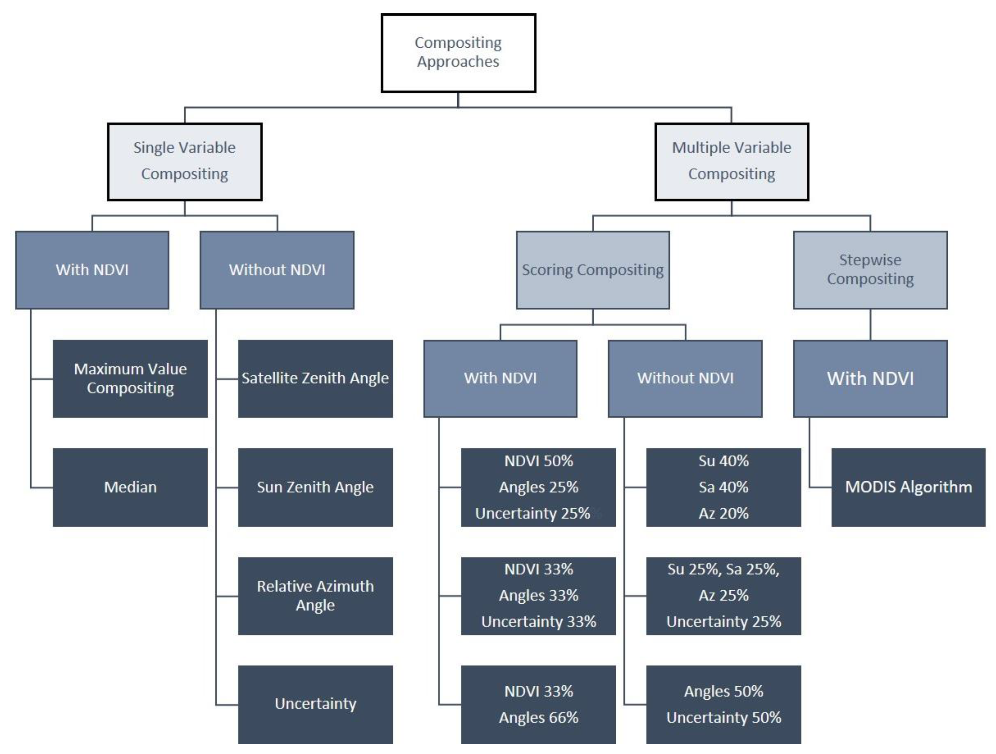
2.3. Compositing Methods

A set of 13 NDVI compositing approaches was tested in this study. Different suggestions and considerations from the literature review have been recognized in the design of the approaches. For example, the intrinsic capability of the NDVI to reduce noise and its behavior to be attenuated by disturbing effects, such as residual clouds, is exploited by using the NDVI value as a criterion for selecting the best observations in many compositing approaches; the MVC is the simplest version of that principle. The influence of the scene geometry, i.e., extreme viewing and illumination angles, leading to distortion effects, was reported by many studies [38,67,110,111], and hence, compositing techniques constraining large zenith angles are included as further options. Furthermore, quality information associated with the pixel reflectance could be considered during compositing. Since compositing based on maximum temperature was reported to result in negatively biased VI metrics [38,40], we did not include this approach.

The basic assumption of this study is that the inclusion of several criteria would lead to better compositing results, as several causes of NDVI over- or underestimation might be eliminated (as, e.g., stated by [38]). However, the magnitude of each of these effects as well as possible interactions are hardly discussed in the literature. Therefore, we designed a range of compositing approaches and compared the results. The aim is on the one hand to better understand the influence of single criteria on the resulting composites, and on the other hand to test the effect of using multiple criteria and thereby of assigning different weights to the compositing criteria. As the calculation of each version required considerable processing power, we chose to test a relatively small set of logical scoring compositing approaches with discrete weight proportions (e.g., making up for one third or half of the weights) instead of performing a “global search” by continuously changing the weight proportions of all variables in small steps. See Figure 3 for a systematic overview and

Table 1. Overview on compositing methods: in the third column, the formula for the score calculation is given, where $S$ is the score, $k$ is each single observation, ${\theta }_i$ is solar zenith angle, ${\theta }_v$ is the view zenith angle, ϕ is the relative azimuth angle, and $A$ is the average acquisition angles score ($A^k=\left(S_{Sa}^k+S_{Su}^k+S_{Az}^k\right)/3$ ).

Approach	Abbreviation	Score Formula	Logic
Single Variable Compositing
With NDVI
Maximum Value Compositing	MVC	$S_{MVC}^k={NDVI}^k$	Established approach: reduces disturbing influences as clouds, snow, and aerosols typically reduce NDVI.
Median	MED	$MED=median\left({NDVI}^k\right)$	Reduces signal attenuating and saturation effects alike.
Without NDVI
Satellite Zenith Angle	Sa	$S_{Sa}^k=\cos \left({\theta }_v^k\right)$	Satellite zenith of 0° (nadir view) is considered best.
Sun Zenith Angle	Su	$S_{Su}^k=\cos \left(\left|{\theta }_i^k-45°\right|\right)$	Illumination of 45° is considered best.
Relative Azimuth Angle	Az	$S_{Az}^k=\cos \left({\varphi }^k\right)$	Relative azimuth angle of 0° is considered best.
Uncertainty	Uc	$S_{Uc}^k=1-{\mathrm{U}\mathrm{c}}^k$	A low uncertainty associated with band 1 + 2 reflectance is considered best.
Multiple Variables Compositing
Scoring Compositing
With NDVI
NDVI 50%          Angles 25%          Uncertainty 25%	NAUc	$S_{NAUc}^k=\frac{\frac{S_{uc}^k+{\mathrm{A}}^k}{2}+{NDVI}^k}{2}$	Half of the weight for score calculation given to NDVI, and ¼ of weight to acquisition angles and uncertainty each.
NDVI 33%          Angles 33%          Uncertainty 33%	NAUc_33	$S_{NAU{c}_{33}}^k=\frac{S_{uc}^k+{\mathrm{A}}^k+{NDVI}^k}{3}$	One third of the weight given to angles, uncertainty, and NDVI.
Angles 66%          NDVI 33%	AN	$S_{AN}^k=\frac{\left({\mathrm{A}}^k\times 2\right)+{NDVI}^k}{3}$	Without uncertainty, 2/3 of weight given to angles, and 1/3 of weight to NDVI.
Without NDVI
Su 40% and Sa 40%          Az 20%	SuSaAz	$S_{SuSaAz}^k=\left(S_{Su}^k\times 0.4\right)+\left(S_{Sa}^k\times 0.4\right)+\left(S_{Az}^k\times 0.2\right)$	Without uncertainty, 1/5 of weight given to relative azimuth, and 2/5 to each zenith angle.
Su 25%, Sa 25%, and Az 25%          Uncertainty 25%	SuSaAzUc	$S_{SuSaAzUc}^k=\frac{S_{Su}^k+S_{Sa}^k+S_{Az}^k+S_{uc}^k}{4}$	Give equal weight to each angle and to uncertainty.
Angles 50%          Uncertainty 50%	AUc	$S^k=\frac{{\mathrm{A}}^k+S_{uc}^k}{2}$	Give half of the weight to angles and to uncertainty each.
Stepwise Compositing
MODIS          Algorithm	MOD	$S_{\left(MVC,\theta \right)}^k=\max \left({\mathsf{\theta }}_v^{S_{MVC}^1},{\theta }_v^{S_{MVC}^2},{\theta }_v^{S_{MVC}^3},{\theta }_v^{S_{MVC}^4}\right)$	Established approach used in the standard MODIS product: used for comparison as a benchmark.

for the method names, abbreviations, formulas, and underlying considerations.

The approaches can be roughly split into single and multiple variable compositing approaches. The single variable compositing approaches comprise on the one hand, methods that rely solely on the NDVI value:

• “MVC”: Maximum Value Compositing. The highest NDVI observation value achieves the highest score, i.e., is selected. This is a standard procedure in image compositing, originally designed for AVHRR compositing (see above). However, studies have shown that MVC selects pixels with large view and solar zenith angles [38,67,110,112]. This is especially true for TOC reflectance [35,113]. The MVC approach thus potentially selects pixels with NDVI greater than the nadir value. Nevertheless, we keep this procedure for comparison reasons.
• “MED”: Median NDVI. The median value of all NDVI observations is selected. This procedure relies on the NDVI values only, and it is thought to reduce signal attenuation effects such as undetected clouds as well saturation or bidirectional reflectance effects, while maintaining an original physical observation.

As it was discussed above that NDVI alone might not be a reliable criterion for composite generation due to bidirectional reflectance effects, we implemented on the other hand single variable compositing methods, which rely on other observation conditions, namely the observation angles and uncertainty measures. Generally, all variable scores span the range of 0–1. The four NDVI-independent single variable compositing methods are included mainly to better understand the influence of these image acquisition conditions on the process of selecting observations.

• “Sa”: Satellite Zenith Angle. The view angle of an observation is used as criterion. As [112] specifies, the directional reflectance factor increases with the off-nadir view angle for any azimuth view direction. Furthermore, the closer an acquisition is to nadir, the lower the effect of atmospheric disturbances is [114]. Hence, previous studies have suggested generating composites approximating images with near-nadir geometry [38,67,110]. Nadir view, i.e., a satellite zenith angle of 0°, is considered best and given highest score while larger angles are given lower scores by ranking the cosine of the satellite zenith angle. Through cosine transformation, an angle of 0° obtains a score of 1, while for example angles of 20°, 40°, or 60°, they obtain scores of 0.93, 0.77, or 0.5, respectively, and a score of 0 is assigned to view angles of 90°.
• “Su”: Sun Zenith Angle. The illumination angle under which an observation is taken is used as selection criterion. An illumination of 45° is considered best (to be in accordance with the TIMELINE BRDF correction, see [12]) and is given the highest score by ranking the cosine of the absolute value of the sun zenith angle minus 45°. The cosine of the absolute, −45°-shifted angle values is in the last step scaled to a range from 0 to 1, resulting in the lowest possible scores of 0 for sun zenith angles of 0° and 90°.
• “Az”: Relative Azimuth Angle. The absolute difference between sun and satellite azimuth angles under which an observation is taken is used as criterion. An equal azimuth angle, i.e., a relative azimuth angle of 0°, is considered best to minimize shadowing effects [112], and is given the highest score by ranking the cosine of the absolute relative azimuth angle, analogous to the scaling of the satellite zenith angle score.
• “Uc”: Uncertainty. The uncertainty value, associated through flags with each pixel in the L2c SDR red and NIR bands and indicating the reflectance uncertainty derived during atmospheric correction, is combined, scaled to 0–1, and used as selection criteria. No uncertainty is considered best and lower uncertainties achieve higher scores through using their reciprocal value.

Based on the behavior of the single variable composites, but also based on the above described literature review and theoretical considerations, a range of multiple variable compositing methods was tested. With the exception of the “MOD” approach (see below), in all of these approaches, the different variables are considered simultaneously. Variable scores are combined according to their weights. Therefore, the NDVI value range of −1 to 1 was linearly rescaled to 0–1. When the acquisition angles (i.e., sun and satellite zenith as well as relative azimuth) are combined through equal weighing in an average score, this is denoted in the following as “Angles”. As for the single variables approaches, one batch of compositing methods includes the NDVI:

• “NAUc”: NDVI, Angles, and Uncertainty. For the score calculation, half of the weight is given to the NDVI value, while ¼ of each is given to the average score of the acquisition angles and to the reflectance uncertainty. In this approach, every available criterion is considered for the selection of the best pixel value, but with an emphasis on NDVI.
• “NAUc_33”: NDVI, Angles, and Uncertainty. For the score calculation, equal weight is given to the NDVI value, to the average score of the acquisition angles, and to the reflectance uncertainty. It is hence conceptually similar to the NAUc approach, but with less influence of the NDVI.
• “AN”: Angles and NDVI. For the score calculation, two thirds of the weight is given to the average score of the acquisition angles, while one third is given to the NDVI value. This approach hence gives higher importance to the acquisition geometry than to NDVI, without considering the uncertainty.

The second group of compositing approaches based on parameter scoring does not include the NDVI:

• “SuSaAz”: Sun Zenith, Satellite Zenith, and Azimuth. In this approach, only the acquisition geometry, i.e., sun and satellite zenith angles as well as relative azimuth angle, is used for compositing. For the score calculation, 40% of the weight is given to each zenith angle, while the relative azimuth is considered with 20%.
• “SuSaAzUc”: Sun Zenith, Satellite Zenith, Azimuth, and Uncertainty. In this approach, every available criterion but NDVI is considered for selecting the best pixel value. For the score calculation, equal weight is given to each of the four parameters.
• “AUc”: Angles and Uncertainty. In this approach, the uncertainty flag is given a relatively high weight. For the score calculation, half of the weight is given to the uncertainty, and half is given to an average score of the acquisition angles.

The approach used for the MODIS 16-day composites relies on the NDVI and view angle. It does not simultaneously integrate them by scoring but it does so in a stepwise procedure:

• “MOD”: MODIS Algorithm. The algorithm first selects the two highest NDVI values and in a second step selects of those the observation with the smaller satellite zenith angle, called CV-MVC algorithm [47,49,107]. Additionally, other studies found this stepwise procedure to be most effective [38]. This standard MODIS procedure is included for comparison reasons as a benchmark. However, we adapted it using the four highest NDVI values as “preselection” to account for the longer integrating period and higher number of input data compared to MODIS.

2.4. Comparison of Compositing Approaches

A range of different criteria was selected to systematically and—where possible—quantitatively compare the compositing approaches, in order to select the algorithm to be finally used for the multi-decadal TIMELINE NDVI generation. Since it was not possible to generate the entire almost 40-year-long time series in 13 versions, this analysis is restricted to data from the year 2007. The year 2007 was a year during which four NOAA missions overlapped (NOAA-12, NOAA-14, NOAA-17, and NOAA-18). This represents the possible diversity of input data to the composites well, especially since these missions carry two different sensor generations (AHVRR/2 and AVHRR/3) [12]. In fact, there are some years (2002, 2003, and 2005), in which data from even five platforms are available simultaneously; however, these mostly include NOAA-15 data, which were excluded from L3 product generation in the TIMELINE project due to unsuccessful data harmonization.

The TIMELINE L3 NDVI product suite consists of three composites: daily, decadal, and monthly. Any selected method should hence be suited for all three intervals. Since more than 95% of the daily composites consist of a maximum of five observations, we do not expect large differences between the compositing methods for the daily composites. Furthermore, we assume that the scientific community relies much more on the decadal and monthly composites. Therefore, we will show some results for the daily composites, but we will focus the visual and statistical analysis mainly on the decadal and monthly products. The conducted evaluation steps are described in the following section.

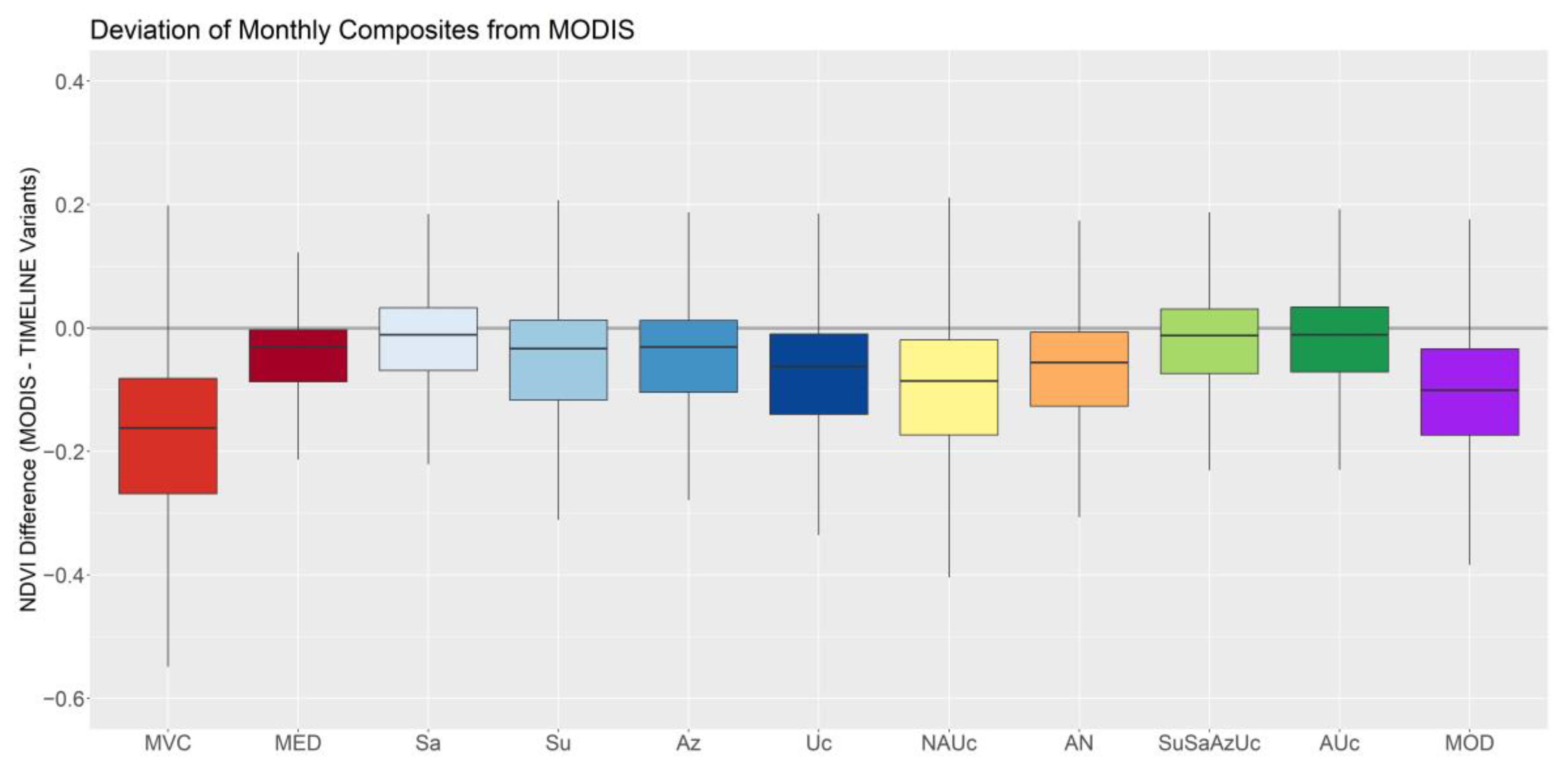
2.4.1. Value Distributions

For all 13 versions of the monthly data sets, the NDVI value ranges and distributions were assessed to analyze the general similarity or biases between the composites. The distribution of solar and satellite zenith angles was also analyzed in this respect. From each monthly composite, a random sample of 100,000 pixels is drawn and aggregated in one yearly data set. The value distributions are then displayed as violin plots, which show the probability density of the data at different values as well as the typical boxplot markers (median, interquartile ranges, minimum, and maximum). Outliers are not plotted.

2.4.2. Spatial Consistency

Spatial consistency and smoothness are vital criteria for composite quality, since sharp bounds in a map might translate to artefacts in thereof derived thematic products. The daily, decadal, and monthly NDVI products have hence been mapped and visually assessed for gaps, signal saturation, and artificial structures resulting, e.g., from scene borders, geometric off-nadir distortions, or data defects. To quantify the general influence of the compositing algorithm on the resulting NDVI, pixel-wise variance as well as maximum NDVI differences between variants were calculated for each product.

For easier comparison, the corresponding MODIS products (MOD13A2 and MOD13A3) are plotted with each composite. Furthermore, the MODIS maps have been used to calculate the deviation of the different monthly composites from MODIS NDVI for all time steps and the entire TIMELINE area. Some focus areas, which stung out partly due to visible artefacts, are shown in more detail: subsets from Central Italy (A), Central Norway (B), Portugal (C), Northern Libya (D), Ukraine and Moldova (E), and Eastern Denmark and South Sweden (F). For the location of the focus areas, see Figure 1.

2.4.3. Temporal Consistency

To ensure temporal consistency of the time series derived from the compositing products, not only single compositing interval maps but temporal NDVI trajectories at selected sites (see Section 2.1) covering a range of different vegetated biomes have been investigated. The time series should be as clean and steady as possible, but also, should reproduce phenological seasonal cycles as well as abrupt events such as harvests. For comparison, the respective MODIS time series at each site is included in the plots, and the deviation of each NDVI variant from MODIS at all stations is calculated in addition.

2.4.4. Spatial Consistency of Acquisition Conditions

As mentioned by [49], compositing methods inevitably result in spatial discontinuities of the generated maps due to the fact that disparate observations can always be chosen for adjacent pixels. As a result, selected pixels may originate from different days, with different viewing and illumination geometries and different atmospheric conditions. As an evaluation criterion, it was therefore suggested that the composite should approximate as much as possible a single-date image with a constant, near-nadir geometry [38]. To evaluate if adjacent pixels have been recorded under similar conditions, we therefore assessed each pixel’s neighborhood conditions in all monthly composites. Using a 3 × 3 moving window, first the number of observation days was counted (i.e., resulting in a value of 1 if all pixels have been recorded on the same day, up to a maximum of 9 if each neighboring pixel of the central pixel was recorded on a different day). In the next step, the variances of the satellite and sun zenith angles in each 3 × 3 moving window have been calculated. All three metrics were analyzed statistically through boxplots and visually by mapping the number of days or variances, respectively, for the TIMELINE study area.

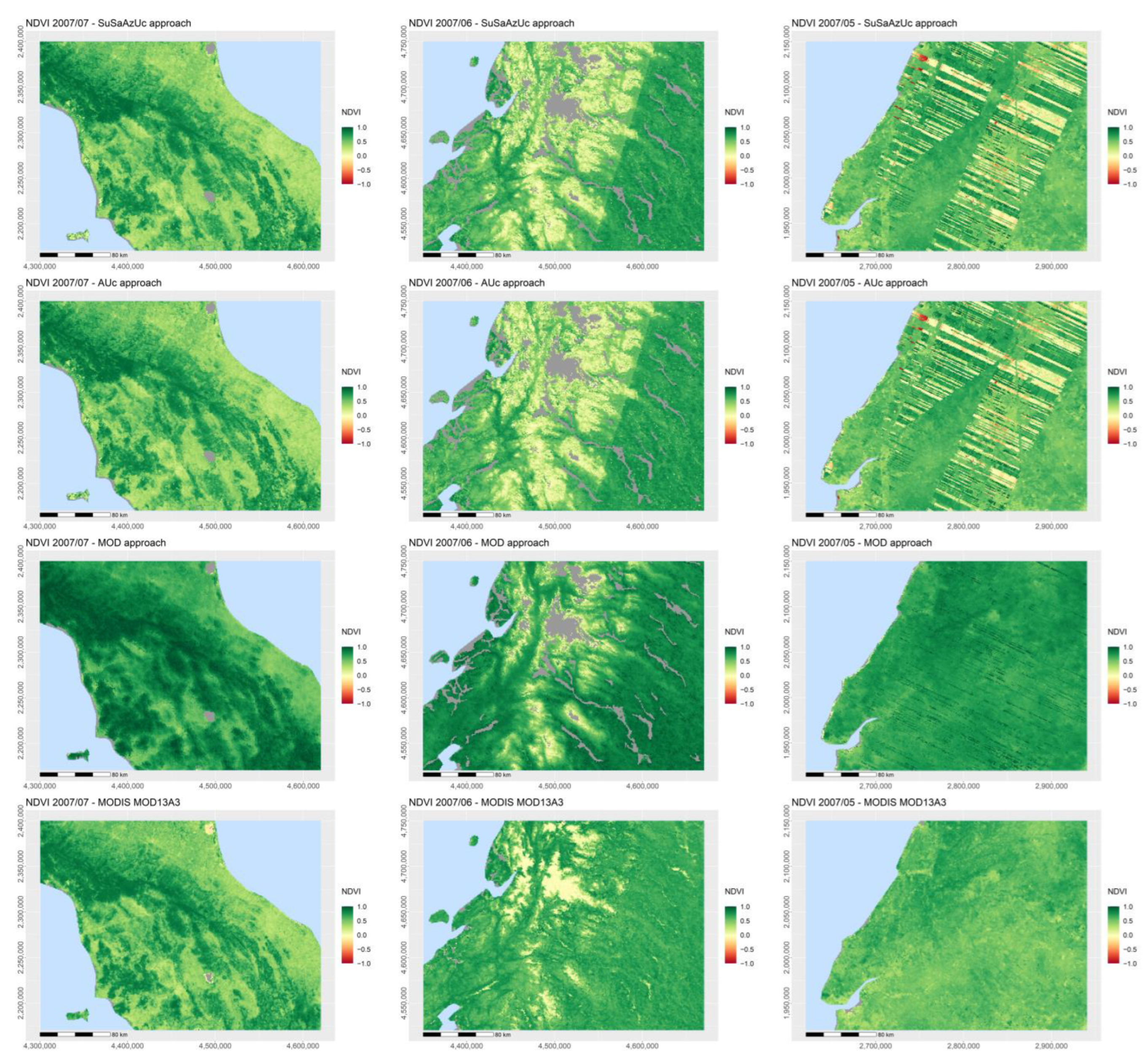
2.4.5. Comparison to MODIS and NOAA CDR NDVI Products

The generated TIMELINE NDVI product for the years 1982–2018 is compared to MODIS and NOAA CDR NDVI products in order to, on the one hand, evaluate the overall quality of the data set, and on the other hand, to investigate how well such time series could be combined. Spatial and temporal consistency with the MODIS products is already analyzed in depth in Section 3.2 and Section 3.3 In Section 5, the match with the entire available time series of the MODIS product, i.e., since 2000, is shown for four selected sites. In addition, the NOAA CDR product for the years 1982–2018 (see Section 2.2.3) is plotted.

3. Results

For the year 2007, 365 daily, 36 decadal, and 12 monthly NDVI composites were produced in 13 variants each. Every composite usually contains four tiles. However, seventy-one daily image tiles and one decadal image tile could not be produced due to missing valid observations, mainly in the winter months and exclusively in the two northern tiles (Figure 1). All compositing variants described in Section 2.3 have been calculated and evaluated according the criteria outlined in Section 2.4. Some variants achieved very different results from the other variants, but some also achieved very similar results. The correlation coefficients and Mean Absolute Difference (MAD) scores of all variants are shown in Table S2. Specifically, within the group of the multiple variables scoring compositing including the NDVI, the NAUc_33 variant achieved similar results with the AN and—to a lesser degree—with the NAUc variant. In the group of the multiple variables scoring compositing without NDVI, SuSaAz resulted in very similar results as the SuSaAzUc and AUc variants. In both cases, not only are the correlation coefficients between the respective scenes very high (≥0.98), but also, the visual and statistical evaluation of the maps and time series revealed high similarities. In order to keep both the length of the manuscript and the readability of the graphs at an acceptable level, the NAUc_33 and SuSaAz variants are not considered in the further description of the results, focusing on the remaining 11 variants.

3.1. NDVI, Satellite, and Sun Zenith Angle Value Distributions

The value distributions of the sampled NDVI values, as well as of the satellite and sun zenith angels, are displayed in Figure 4. They show partly distinct differences between the compositing approaches. Regarding the NDVI distribution (Figure 4, top), the MVC approach clearly stands out and generates the highest values overall, with a very high median value of 0.70. A tendency toward value saturation is clearly visible and most pronounced during the summer months, with the median and 75th percentile at 0.81 and 0.93, respectively. The other variants show fewer differences, especially regarding their NDVI distribution shape. The MED NDVI approach expectedly results in overall lower values than MVC (median of 0.51), with no saturation, a more natural data distribution, and a relatively narrow range of low NDVI values. Out of the four single variable composites, the versions solely relying of the sun and sensor angles Sa, Su, and Az, generate overall similar value distributions with low median values (0.45, 0.49, and 0.48, respectively). Accordingly, the SuSaAzUc and AUc approaches, weighing the angles with 75% and 50%, result in similar NDVI value distributions (median of 0.45 and 0.43). The behavior of the Uc criterion is not consistent, since the single variable approach employing Uc alone results (with a median of 0.53) in higher values than the Su, Sa, or Az approaches, but also than the SuSaAzUc and AUc approaches, in which it is used together with the angles criteria. The NAUc approach, giving half of the weight to NDVI and one quarter each to angles and uncertainty, achieves the second highest NDVI values (median of 0.62) after MVC, followed by the other variants, which include the absolute NDVI values in the weight generation, i.e., MOD, employing high NDVI as the first selection criteria (median of 0.59), and AN, giving one third of the weights to NDVI, with an accordingly lower median value (0.55). This pattern is also the same when the different seasons are investigated (not shown).

Regarding the satellite zenith angle distribution (Figure 4, middle), the Sa variant stands out with a median of 3.53 degree. As a small view angle was the sole criterion in this approach, this was to be expected. Accordingly, other variants that include the satellite zenith angle in their weighing approach to a large degree, such as SuSaAzUc, AUc, and AN, result in median view angles below 15 degrees and value distributions that are clearly biased toward low values. The variants NAUc and MOD, which employ the (view) angles criterion by at least 33%, result in similar value distributions, balanced but with a bias toward small satellite zenith angles (medians of 20.4 and 22.0, respectively), while the purely NDVI-based approaches, MVC and MED, select observations made under very large satellite zenith angles (medians of 48.0 and 32.3, respectively). The Su and Az variants show very similar value distributions with a strong bias toward high values (medians of 44.1 and 44.3), which might originate from the orbit and sensor characteristics of the AVHRR series. Its wide swath generates in every scene large satellite zenith angles. Since the sun zenith is a factor changing mainly in north–south direction, while the view zenith varies mainly in the east–west direction, large satellite zenith angles are sampled with equal probability as nadir view observations if an illumination angle of 45° is the only pixel selection criterion. The sun zenith angle distribution (Figure 4, bottom) is hardly influenced by the choice of the compositing procedure. Most variants have a very similar, uniform probability density distribution of sun zenith angles, biased toward higher values, with median values of 49.4 ± 1 degree. Only the Su approach deviates from this pattern, showing a normal distribution centered around a median of 45.6 degrees. As a sun zenith angle of ideally 45° was the sole criterion in this approach, the distribution of the sun zenith angles in the Su variant reflects the underlying compositing rules.

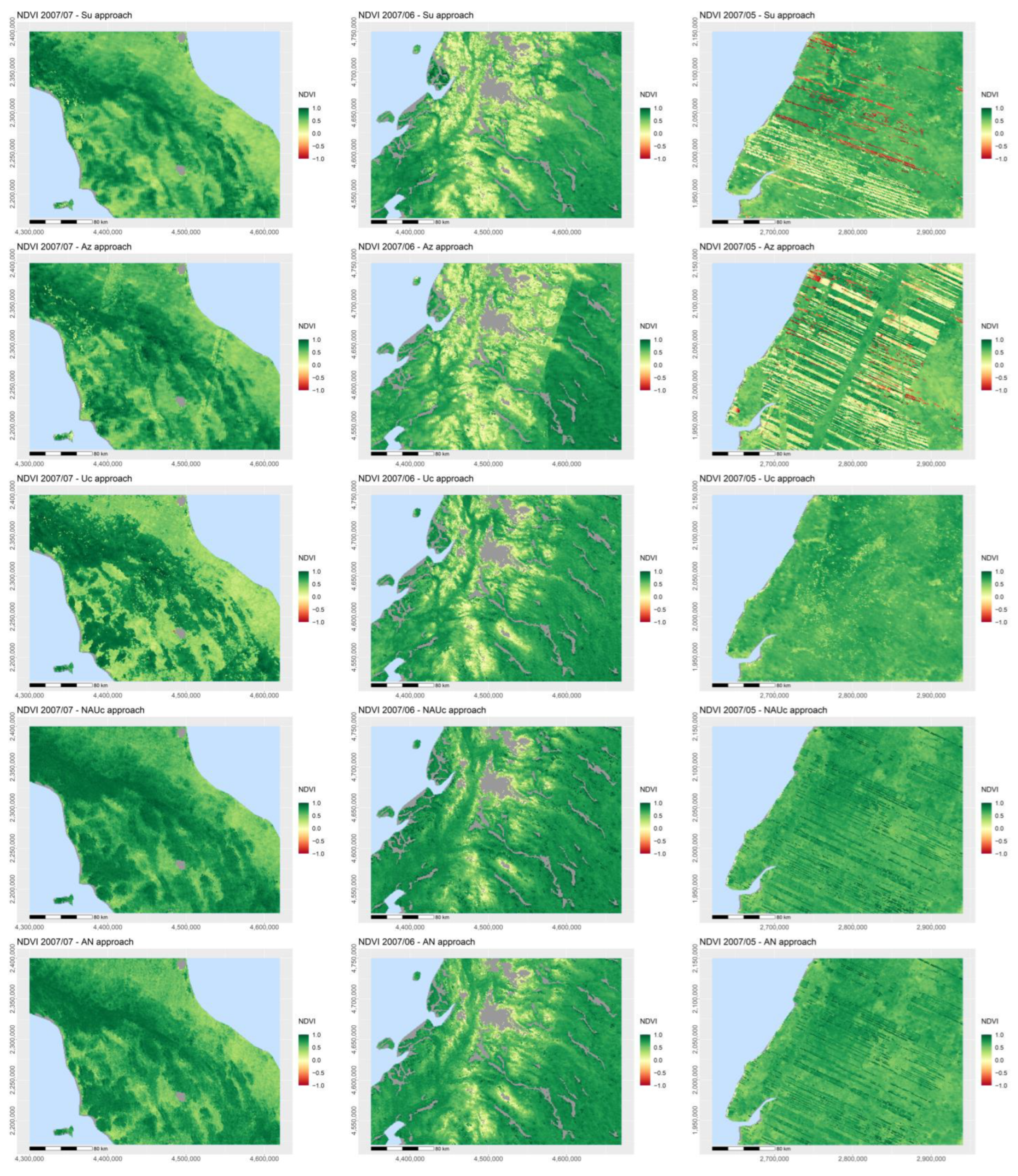
3.2. Spatial Consistency

Figure 5 displays the monthly NDVI maps for the TIMELINE extent in May 2007 based on the different compositing approaches. Compared to the other compositing approaches as well as to the monthly MODIS product (bottom right tile), the MVC compositing approach (left tile in the first row) displays consistently higher values, even in northern latitudes and over non-vegetated areas (most prominently the desert areas of Northern Africa). Uniform planes of high NDVI values indicate that mainly pixels affected by signal saturation have been selected. Furthermore, artefacts that become visible as stripes and edges can be identified in the otherwise homogeneous desert areas. Although also being based on the NDVI as selection criteria only, the MED approach (right tile in first row) seemingly generates very smooth maps. While the vegetation patterns are quite similar to the MODIS product and natural structures, such as mountain ranges or natural gradients, can be well recognized, no artificial bounds are discernible.

The three purely angle-based variants Sa, Su (second row), and Az (left tile in the third row) all exhibit different, but noticeable geometric artefacts. In the Sa map, edges of the north–south-oriented view angle stripes following the usual orbital passes can be seen, most clearly over the deserts and in Easter and South-Eastern Europe. This is especially prominent in winter and spring composites (not shown). In the Su approach map, artefacts are less obvious on the continental scale, but discernible as smaller stripy patterns over the Iberian Peninsula, the Baltics, and in the Balkans and Greece. Both effects, i.e., stripy patterns over Portugal, Eastern Europe, and the Balkan, as well as the north–south-oriented border effects following satellite orbits from the Baltics to North Africa, influence the Az approach map (left tile in third row). The Uc approach (third row, right tile) generates maps that seem smooth on a continental scale, with clearly visible distinct natural structures. However, especially during the winter and spring months, artificial structures that relate to scene boundaries are visible (not shown) as well as small scale patches of negative values (in the shown example, e.g., in the Bosporus region), which affect the consistency of the maps.

The multiple variable composites including NDVI (NAUc and AN, fourth row) result in similar monthly composites, which seem to be affected by geometric artefacts to a lower degree. Only over the deserts of North Africa are stripes and edges clearly visible. While showing similar patterns as the MODIS products, the NDVI values are overall relatively high, making natural features such as mountain ranges less discernible. The two variants not including the NDVI in the selection criterion (SaSuAzUc and AUc, fifth row) are again more strongly affected by geometric artefacts in the form of north–south-oriented striping and smaller scale horizontal striping induced by strongly negative values. These effects are clearly visible in both maps, e.g., over the desert areas, the Iberian Peninsula, Eastern Europe, and the Bosporus. Nevertheless, apart from the introduced noise, the overall NDVI value distribution seem to be in the range of the MODIS product. The actual MOD variant (bottom row, left tile), however, strongly overestimates the MODIS product and while not showing any strong geometric artefacts and depicting natural gradients well, it is clearly afflicted by signal saturation, similarly to the MVC approach.

The comparison of the NDVI maps and the identified differences among them indicate the strong influence of the compositing approach on the resulting NDVI maps. To quantify this impression, the pixel-wise variance between compositing approaches as well as the maximum difference in NDVI have been calculated. As an example, the variance and maximum NDVI difference for the monthly composite of April 2007 is shown in Figure S2. It can be seen that variance is not homogenous throughout the study area, but it is especially high in the northern and eastern parts of Europe (in this case probably due to the reduced number of valid observations because of snow and clouds), the Balkans, Turkey, and regions of high vegetation density, such as the Nile delta. The map indicating the range of derived NDVI values through different compositing approaches highlights that pixel-wise NDVI can deviate up to a difference of 0.6 NDVI (on average 0.3 NDVI). However, in the summer months, with overall higher NDVI values, the differences are smaller (not shown).

Figure 6 summarizes the above made observations on the accordance of the compositing variants with MODIS by displaying the average deviation of the monthly composites from MODIS NDVI. Since all the boxplot medians are negative, Figure 6 shows that all AVHRR-based composites are biased toward higher values than the MODIS product.

However, differences between the approaches exist. As could already be seen from the spatial maps, NAUc, MOD, and most prominently, the MVC approach show significantly higher NDVI values than the MODIS product as well as a large interquartile range, indicating that the differences are not systematic. Uc and AN also overestimate MODIS on average by 0.06 NDVI. Sa, SuSaAzUc, and AUc feature the smallest deviance from MODIS (median deviation around 0.01 NDVI). The MED approach results in the smallest range of deviations, indicating that the patterns of MODIS are nicely reproduced, although with a small offset (median deviation 0.03 NDVI).

Figures S3 and S4 visualize the continental scale NDVI maps for decade 2 of October 2007 (i.e., 11 October–20 October 2007) and 23 June 2007, respectively, as examples for decadal and daily products based on the different compositing approaches. At first glance, these maps show that the spatial coverage of the decadal and daily maps is not as exhaustive as the monthly product. These time intervals obviously are not long enough to collect sufficient valid observations to map NDVI for the entire study area. Apart from this difference, most issues observed with each compositing method in the monthly composites are also traceable in the shorter-term composites. The MVC and MOD approaches generate spatially consistent decadal maps, which, however, show very high NDVI values for the largest parts of Europe (Figure S3, left tiles in top and bottom rows). Synthetic geometrical structures are only discernible over desert areas and large plains in Eastern Europe. Additionally, the MED algorithm results in a smooth and differentiated decadal map in which no artefacts are visible.

In the decadal Sa maps however, the north–south-oriented striping is still present but is less prominent than in the monthly composites, especially in the summer months. The same is true for the decadal Su maps, in which, especially the issue of horizontal stripes of strongly negative values is reduced. Here, the shorter integration interval seems to reduce the variance introduced through viewing and illumination geometry. However, both variants appear visually noisier. For the decadal Az and Uc composites, similar artefacts prevail as in the respective monthly data sets. Accordingly, the decadal SaSuAzUc and AUc maps have geometric artefacts in the form of north–south-oriented striping and smaller scale horizontal striping, especially in some spring and early summer scenes. The decadal NAUc maps seem to be only rarely affected by geometric effects, but have overall relatively high values as well as noisy patches of high NDVI, which are not continuous or relatable to any natural landscape features. The decadal AN maps show similar properties as the NAUc maps, but with generally lower NDVI values and less saturation patches. Furthermore, this specific example also shows that the MODIS product (right tile of bottom row), which is usually very spatially consistent, is sometimes affected by large scale artefacts (in this case, in North-Eastern Europe).

Figure S4 shows the daily NDVI maps from 23 June 2007, based on the different compositing approaches. Comparison of the maps reveals that the differences between the tested compositing approaches are minimal for the daily composites. Value ranges and landscape patterns are overall the same, with the rare but largest differences being introduced by geometric artefacts (in the given daily maps, e.g., the wedge-like patch of high NDVI values in Turkey being present in the Az, MED, MVC, NAUc, and Uc variants) and patchy saturation areas.

On the continental scale, identifying small scale artefacts and finer deviations is difficult. Therefore, the monthly NDVI maps based on the different compositing approaches are shown in the focus areas A–C (Figure 7) and D–F (Figure S5). Area A displays Central Italy, which is characterized by a hilly landscape covered by a mosaic of forests (especially at higher elevations) and agriculture. Typical compositing errors that have partly been described above and that can be observed in these subsets are signal saturation (MVC, Uc, and MOD composites) and geometry effects such as visible orbit edges (e.g., Az and AUc). In addition, on that scale another geometry issue becomes visible: pixel distortions (north–south-oriented blurring) in the Su composite, which is probably caused by the selection of far-off-nadir observations once the view angle is no longer a selection criterion. The MED and AN maps are the spatially most continuous products.

Focus area B, which is located in Central Norway, is a typical mountainous fjord landscape covered by evergreen forests and herbaceous vegetation. As expected, geometry issues are especially prominent at such high latitude. Orbit edges are visible in the Az, SuSaAzUc, and AUc maps, and pixel distortions are visible in the Su and Az maps. Furthermore, due to the patchy landscape and the lower availability of valid observations, maps are generally quite noisy (e.g., MVC, MOD, Sa, NAUc, and AUc composites). Focus area C covers Central Portugal, north of Lisbon. The Mediterranean landscape is dominated by sparse sclerophyllous forest intermixed with cropland in the lowlands, herbaceous cover, and shrubland. In the selected subset, especially the occurrence of horizontal stripy patterns is visualized. The MVC, Su, Az, NAUc, AN, SuSaAzUc, AUc, and MOD composites are all affected to a stronger or weaker degree. In addition, orbit edge artefacts can be seen in the Sa approach map. Hence, only the MED and Uc maps in this example are without geometric issues.

The focus areas displayed in Figure S5 highlight some additional detected issues in the NDVI composites. Focus area D is located in Northern Libya, west of Tobruk, covered mainly by a flat vegetation-free sand desert. Only in the north-west, the al-Dschabal al-Achdar highland is covered by forest, shrubland, and cropland. Due to the very homogeneous surface of the desert area, the geometric artefacts can be visualized. While in the Sa approach the orbit edges prevail, in the Su approach, the problem of integrating different illumination conditions can be investigated. The Az approach shows issues with horizontal bounds. Accordingly, the NAUc, AN, SuSaAzUc, and AUc approaches, which integrate the angle constraints, show combinations of these effects. MVC and MOD are without geometric structures, but show too high values.

Focus areas E (covering a large cropland plain in Southern Ukraine and Moldova) and F (covering cropland areas and forests in Eastern Denmark and South Sweden) both include examples of high salt-and-pepper noise (SuSaAzUc, AUc, and MOD maps in subset E; Sa, Su, Uc, SuSaAzUc, AUc, and MOD maps in subset F) as well as noisy patches of high NDVI, which do not relate to any natural landscape features (MVC and NAUc maps in subset E). In addition, geometry issues can be seen in the Sa and Su maps of focus area E and in the Az maps of focus area F.

3.3. Temporal Consistency

The time series’ of the different compositing approaches for 2007 have been plotted for all 37 stations. In Figure 8, the daily (top row), decadal (middle row), and monthly (bottom row) composite time series are shown for three selected sites: the desert site Algeria5, the deciduous broadleaf forest site Hesse, and the agriculture site Piedmont. For details on the sites, see Figure S1, and for a less cluttered, split-up version of Figure 8, see Figure S6.

In general, the daily plots (top row) show at the one hand the low influence that the compositing scheme has on the resulting NDVI map if only few observations are to be combined (with most points in a time series being plotted on top of each other), and on the other hand, they show the high variability that a daily AVHRR data set inevitably exhibits. Nevertheless, the characteristics of the different land-cover types are generally reproduced, with no vegetation signal over the desert site (left), overall high NDVI levels and an NDVI increase during summer over the forest site (middle), and the very distinct phenological cycle of the rice cultures on the agricultural site (right). On top of each plot, the MAD of the compositing variant from the MODIS time series is included in the plot legend. It can be seen that over the desert sites, variations between composites are minimal. The time series’ closest to MODIS are Sa, AUc, and MOD (MAD: 0.019), and the composites deviating the most are MVC (MAD: 0.033), NAUc (MAD: 0.026), and Uc (MAD: 0.024). On the forest site, the variants that are best at approximating MODIS are SuSaAzUc (MAD: 0.070), AUc (MAD: 0.075), and Az and AN (MAD: 0.076). The largest deviations are observed for MVC (MAD: 0.097), Su (MAD: 0.094), and Uc (MAD: 0.087). On the agriculture site, SuSaAzUc (MAD: 0.06), AUc (MAD: 0.064), and SA and MOD (MAD: 0.065) fit best to the MODIS curve, while again, MVC (MAD: 0.084), MED, and Su (both MAD: 0.075) deviate the most. Enlarging the compositing interval to 10 days (middle row) already enables an almost continuous time series for most sites. On the desert site (left), stable bare soil trajectories are generated for most approaches, with only MVC, Az, NAUc, AN, AUc, and MOD including too high values in the first half of the year. Accordingly, these are the variants that reach high MADs above 0.04. On the Hesse forest site, the phenological cycle of green-up, peak of season, and senescence between March and October are overall well captured, while the February and November composites are very noisy and the January and December observations are missing completely. Looking at the stability of the individual variant time series, the MED, Az, Uc, and AN approaches generate a rather stable time series, while the others are rather volatile. Statistically, the best variants on this site are the MED (MAD: 0.076), Az (MAD: 0.078), and AN (MAD: 0.079) approaches, while all other approaches have MAD > 0.08, with the MVC being off the most (MAD: 0.132). The phenological cycle of the rice cultivation site in Piedmont is overall captured well, although the winter and spring phases also on this site are very noisy, and the green-up seems to be detected too late by 10–20 days in comparison to the MODIS observation. Regarding the time series consistency, the Sa, Uc, SuSaAzUc, AUc, and MED approaches are rather stable, while the Su, Az, NAUc, AN, MVC, and MOD feature more and larger random jumps. The highest accordance with MODIS is achieved again by the MED algorithm (MAD: 0.076), as well as by the Sa (MOD: 0.079) and the SuSaAzUc (MOD: 0.08) approaches.

The time series’ of the monthly composites (bottom row) are the most continuous data sets. On the desert site, the picture is largely the same as for the decadal time series. Additionally, in these intervals, some approaches such as MVC, NAUc, AN, SuSaAzUc, AUc, and MOD select too high NDVI values for their composites and hence yield MADs ≥ 0.045. The MED (MAD: 0.012), the Sa (MAD: 0.027), and the Uc (MAD: 0.028) approaches reach the highest accordance with MODIS on this site. On the forest site (middle), a continuous time series could be generated from February to November. Closing the gaps however introduced some variance to some of the different compositing variants. Especially the Sa, Uc, AN, SuSaAzUc, AUc, and MVC time series’, which are all rather jumpy. In addition, while the MVC variant (MAD: 0.154) continuously overestimates the MODIS time series, variants such as SuSaAzUc (MAD: 0.11), AUc (MAD: 0.107), and Sa (MAD: 0.08) rather underestimate the forest NDVI during the mid of season.

While still being a bit too flat in comparison to MODIS, the MED (MAD: 0.06), Az (MAD: 0.065), and MOD (MAD: 0.076) time series’ approximate it best. A certain variance between the compositing approaches is also observable on the agricultural site (right), but the phenological shape is still well captured in most of them. Only the Su, NAUc, SuSaAzUc, and AUc variants do not reproduce the temporal vegetation growing pattern very well. In comparison to the monthly MODIS product, also the timing of green-up and harvest seem to be well approximated. The closest fit was achieved by the Az (MAD: 0.055), MED (MAD: 0.057), and Uc (MAD: 0.067) approaches, while the MVC (MAD: 0.166), Su (MAD: 0.105), and NAUc (MAD: 0.101) showed the largest deviations.

Evaluating just these three sites made it clear that although some variants are systematically off in comparison to the MODIS time series (such as MVC or NAUc), there is no clear pattern for the other variants. For example, AUc or MOD in some cases are close to the MODIS reference, but far off on other sites. Therefore, the deviation of the monthly (Figure 9), decadal (Figure S7), and daily (Figure S8) composites over all stations was calculated. Figure 9 shows that the Sa, SuSaAzUc, and AUc time series are numerically closest to the MODIS time series. Additionally, the MED and the Az variants overestimate the MODIS reference only slightly, while MVC, NAUc, and MOD deviate strongly. For the decadal composites (Figure S7), this pattern is similar, but the differences between the variants are smaller, as is the overall deviation from the MODIS time series. For the daily composites, (Figure S8), the differences are only marginal, which is consistent with the visual interpretation of the time series plots.

3.4. Spatial Consistency of Acquisition Conditions

To assess the spatial continuity of the generated maps with regard to the image acquisition conditions, the variance of the day of acquisition, the satellite zenith angle, and the sun zenith angle have been calculated in a 3 × 3 moving window for each compositing approach. Figure 10 (top) shows the boxplots of the DOY variance for each approach. MED shows the highest variants with a median of 5 (i.e., meaning that, on average, the 9 pixels in the moving window have been recorded on 5 different days), followed by MVC, NAUc, and MOD, with a median of 3 days. All variants that give high weight to viewing or illumination angles (Sa, Su, Az, SuSaAzUc, and AUc) achieve the lowest variance with a majority of all pixels being recorded during the same day. This is logical, since the emphasis of the acquisition geometry favors the selection of all pixels from one image swath. These differences also become visually apparent in the variance maps of May 2007 of each approach (Figure S9, left column), in which the aforementioned geometry-scoring approaches appear mostly in dark blue colors (representing a variance of 1 DOY). The MED approach stands out with overall high DOY variance values.

The same overall pattern is also visible in the satellite (Figure 10, middle) and sun zenith angle (Figure 10, bottom) variance boxplots. MED has the highest variance in the viewing and illumination zenith angles among adjacent pixels, followed by MVC, MOD, and NAUc, i.e., all variants that give at least 50% of the scoring weight to NDVI. The Su approach shows the smallest variance for both zenith angles, followed by SuSaAzUc, Sa, Az, and AUc. Accordingly, also the variance maps of satellite and sun zenith (Figure S9, middle and right column) follow the above described pattern. From these variables, it can also be seen that variance is spatially random where it is high, but it rather systematically depends on the image swath borders, e.g., in the case of the otherwise very homogeneous Az approach.

4. Discussion

The conducted analyses demonstrate the tremendous influence of compositing procedures on the resulting AVHRR NDVI composites, especially when longer intervals are envisaged (as the monthly composites in this study). Furthermore, the performances of the different approaches varied for some variants, strongly depending on the evaluation criterion considered. The selection of an algorithm therefore must consider a range of aspects, which is discussed in the following subsections for each compositing approach/group of approaches and summarized in

Table 2. Evaluation of compositing methods based on different criteria. If a criterion is well or very well fulfilled, it is marked with pluses (+/++); if a criterion is partly or completely unfulfilled, it is marked with minuses (-/--).

	Criteria	Value Distribution	Spatial Consistency	Spatial Match to MODIS	Time Series Consistency	Time Series Match to MODIS	Neighborhood
Approach
MVC		--	-	--	-	--	-
MED		+	++	+	+	+	-
Sa		++	--	++	-	++	++
Su		+	-	+	--	-	++
Az		+	--	+	-	+	++
Uc		++	-	-	+	-	+
NAUc		-	+	--	--	--	-
AN		+	+	-	+	-	+
SuSaAzUc		++	--	++	-	++	++
AUc		++	--	++	-	++	++
MOD		-	-	--	--	--	-

.

4.1. Purely NDVI-Based Approaches: MVC and MED

MVC compositing historically was the first approach used for NDVI compositing, originally designed for AVHRR data. However, all conducted analyses in this study point out the main issue introduced by the MVC approach: biased NDVI value distributions that indicate the selection of observations affected by signal saturation. This leads to a general NDVI overestimation, even in sparsely or non-vegetated areas, and a large mismatch with MODIS, both at the investigated stations and for the entire study area. In addition, artefacts such as stripes and swath edges do occur in the MVC products. These findings are in accordance with the literature. It was reported that the MVC preferentially selects pixels from off-nadir angles [110,111,114,115], especially from the forward scattering direction where pixels have higher NDVI. The higher NDVI in forescatter geometry is attributed to two effects related to anisotropy: in off-nadir direction, the sensor views (a) a higher proportion of the more NIR reflective vegetation and a lower proportion of the less reflective soil, thus increasing the NDVI ratio value, and (b) a higher proportion of vegetation components in the upper layers of the canopy, which scatter a higher proportion of solar incident flux [38,112]. Furthermore, the MVC approach was designed for TOA data, and it was reported early that the NDVI overestimation effect is especially true for TOC reflectance [35,113]. Since we employ atmospherically corrected data, this issue affects the results of the MVC approach strongly. Accordingly, the MVC achieves negative valuations in each evaluation category (see Table 2).

In contrast to the MVC approach, the MED variant results in balanced value distributions and generates very smooth and consistent maps, while small landscape features are still discernible. The MED approach in fact is the only approach that did not show any geometric artefacts, leading to a “++” valuation of this criterion (see Table 2). The spatial match with the MODIS products is—with a median deviation of 0.03 NDVI—not as close as in other variants (e.g., Sa, SuSaAzUc, and AUc, see below), but shows the smallest range of deviations, indicating that the patterns of MODIS are well reproduced. Looking at the temporal consistency, the MED approach is among the best approaches, generating stable time series with few unnatural jumps. Accordingly, also in the time series comparison to MODIS, MED is among the variants with a close match to MODIS. The only weakness detected for the MED approach is the high heterogeneity when investigating the neighborhood acquisition conditions. The approach clearly stands out with high variances in DOY, satellite, and sun zenith angles within a 3 × 3 window. This indicates that a majority of the selected NDVI observations have been collected under differing conditions than the neighboring ones. Unexpectedly, this does however not compromise the spatial consistency of the MED maps, as mentioned above. This might be caused by the aspect that especially if many good quality observations are available, the NDVI values among which the median is selected are very similar. Hence, the selection of an observation with the according DOY and geometries is more randomized than for other approaches, as minimal differences in the NDVI might already induce a different selection. The ideal of a single-date image with a constant geometry is therewith not fulfilled. However, apart from this theoretical consideration, this circumstance does not seem to hamper the spatial or temporal consistency of the product, and hence will not affect any application based thereon. This criterion is therefore marked as only partly unfulfilled in Table 2.

In the literature, median compositing is usually only used for combining high spatial resolution data such as Landsat or Sentinel-2 [41,44,45,46]. Thereby, the aim is mostly the generation of gap-free multi-spectral mosaics that are representative of long time periods (seasons or years), while no composite time series at high frequency intervals (such as weeks or months) were generated using this approach. The mosaics serve in most studies as a basis for land-cover classification and change detection, not for time series analysis. One reason why median compositing so far was not used on AVHRR data might be the susceptibility of the approach to undetected clouds or missing atmospheric correction. Since we can rely on a thorough preprocessing chain in the TIMELINE project, the used surface reflectance is robust and mostly unaffected by disturbing influences, enabling the excellent performance of such a simple statistical approach.

4.2. Purely Geometry-Based Approaches: Sa, Su, and Az

The purely geometry-based approaches Sa, Su, and Az were included in this analysis to better understand the influence of the scene geometry on NDVI mapping. In contrast to [113], composites closely resembling a nadir image on a pixel basis could be generated. However, this by itself did not guarantee a stable and artefact-free NDVI time series. While all three approaches achieved satisfyingly balanced NDVI value distributions, they are all strongly affected by geometric artefacts, especially the Sa and Az approaches. Sharp edges of north–south-oriented image swaths, smaller stripy patterns that might be introduced by sensor defects, or pixel distortions (north–south-oriented blurring) caused by far-off-nadir observation could be found in many composites. This was partly expected, as changes in the “best” viewing and illumination angles per definition must be abrupt. Nevertheless, this analysis also illustrates some issues that have not been prominently discussed in the literature, and highlights the importance of carefully selecting weights assigned to sensor or sun angles when used in multiple variable compositing (see below). Looking at the time series consistency, the three approaches mostly result in a rather volatile time series. In comparison to the MODIS NDVI values, the Sa, Su, and Az approaches achieved overall close matches and good ratings (Table 2), probably due to the dampening effect of near-nadir observations with regard to a signal saturation. Additionally, naturally, the neighborhood analysis revealed very homogeneous acquisition conditions most closely resembling single-date image with constant geometry. However, given the high influence that persistent geometric artefacts in a multi-decadal time series product would have on any kind of spatial analysis, these positive ratings cannot counterbalance the above described issues with spatial inconsistencies. The usage of data corrected for bidirectional effects might mitigate these problems [38], but such corrections have proven difficult and might introduce new types of artefacts or blur spatial and temporal features.

4.3. Uncertainty Information as Sole Selection Criterion: Uc

Using only the uncertainty information derived from the TIMELINE atmospheric correction for the best-pixel selection was a rather explorative approach, for which no reference could be found in the literature (probably due to the lack of such additional information in most data sets). The approach performed well in some regards, such as the generation of balanced value distributions, stable time series at the station sites, and relatively homogeneous neighborhood conditions. The latter is probably caused by the fact that atmospheric conditions do not change on the small scale, hence neighboring pixels are probably flagged with similar uncertainties. However, the spatial consistency of the Uc maps are compromitted by orbit bound artefacts, signal saturation, as well as small scale patches of negative values. At least, the issue of horizontal striping seems to be caught by using the uncertainty criterion (see Figure 7), which proves the general benefit of the uncertainty information in image composition. Nevertheless, the bad spatial and temporal matches to the MODIS product are further aspects reducing the valuation of the Uc variant.

4.4. Multiple Variable Compositing Not including NDVI: SuSaAzUc and AUc

The above described analysis of the single variable compositing approaches Sa, Su, Az, and Uc already summarizes the immanent strengths and weaknesses of the approaches that are reproduced and partly reinforced in the multiple variable compositing relying on these criteria, namely SuSaAzUc and AUc. Through penalizing large satellite and sun zenith angles as well as unfavorable azimuth viewing/illumination conditions or uncertainty flags, most observations made under moderate geometric conditions are selected. This leads to balanced value distributions, and through the avoidance of very high NDVI values, to a close overall match to the MODIS product. However, both of the SuSaAzUc and AUc approaches lack spatial and temporal consistency. Especially, geometric artefacts render the variants unusable. While some distortions such as pixel blurring are in fact avoided through the combined weight of different angles, other effects such as sharp borders and the striping of noise persist. Time series consistency is affected by random jumps and NDVI overestimation (see, e.g., the green lines in the desert and forest site plots of Figure 8).

4.5. Multiple Variable Compositing including NDVI: NAUc and AN

The issues in the SuSaAzUc and AUc data sets not including NDVI (see Section 4.4) indicate that not considering the absolute value of NDVI in a compositing approach introduces problems that cannot be counterbalanced. On the other hand, the sole use of the maximum NDVI did not achieve satisfying results either (Section 4.1). Using both aspects as the quality criteria, either as weights in the NAUc and AN variant or stepwise in the MOD variant (see Section 4.6), seems to be a promising approach. In fact, the spatial consistency of the NAUc and AN approaches is satisfying, with geometric artefacts occurring considerably more seldom than in most other approaches. However, the conducted tests also show that the assignment of weights thereby plays and important role, as the results of both approaches partly diverge strongly. For example, with the weight of the NDVI in the NAUc approach being 50% and of the angles being only 25%, it produces the on average second highest NDVI values of all the approaches (see Figure 4), while the median NDVI of AN with an NDVI weight of only 33% and angles weight of 66% is in the range of the other approaches. Similarly, differences in the temporal consistency could be observed between the two variants. The AN time series’ at the stations are overall more stable and have smaller MAD values when compared to MODIS. Looking at the stations but also at the continental maps, both variants show an insufficient match to the MODIS time series, with the NAUc algorithm however deviating more strongly, indicating again that the selection of weights, and thereby, probably the low overall weight of the sun and satellite angles (25%), were not favorable. It can be hence derived that in general, combining the NDVI and other restrictions in one score for a best-pixel selection can reduce, e.g., geometric effects. However, a high enough weight of the illumination and viewing angles seems to be crucial for satisfying composite consistency.

4.6. Imitating the MODIS Standard Product: MOD

The MOD algorithm was included in this study with the aim to approximate the standard MODIS NDVI product. However, surprisingly, no close agreement to MODIS products could be found, neither on the continental scale nor when looking at the time series. Like the MVC approach, the MOD approach generates overall high values, is also affected by saturation effects, and strongly overestimates the MODIS reference. In addition, the MOD time series’ are mostly inconsistent as they include noise and jumps. We did not expect this result, since it was found in earlier studies that, among the tested criteria, the maximum NDVI in combination with the minimum view angle was the most effective two-step criteria [38]. We therefore assume that, while we already considered the large differences in MODIS and AVHRR NDVI input data generation and compositing intervals through the usage of the four highest NDVI values as “preselection” as compared to only two in the MODIS approach (see Section 2.3), the algorithm would still need to be further adapted to the specific TIMELINE L2 SDR AVHRR characteristics to achieve more similar results.

4.7. Algorithm Selection, Limitations, and Further Work

In Table 2, the eleven variants are evaluated according to the six criteria that were assessed in this study. If a variant performs well or very well in one aspect, it is marked by a plus or two pluses, respectively. Accordingly, if saturation, artefacts, or inconsistencies could be observed in the different data set versions, they are marked with minuses. Thereby, a double minus mark is meant to identify problems with a data set that seriously compromises the usability of the time series, even if it performs well in other regards. For example, strong geometric artefacts such as striping would inevitably affect any spatial analysis and could not be counterbalanced by a realistic value distribution or smooth time series behavior (see, e.g., Section 4.2) This kind of marking enables an objective method selection, which resulted in the MED approach being chosen as the best-performing algorithm (Table 2). The AN variant thereby ranges as the “second-best” approach, which could further be refined in the future (see below).

This systematic procedure emphasizes that a compositing approach might perform well in certain aspects, but can show substantial limitations when looking at others. Similarly, large differences in the evaluation of compositing approaches were also observed by [41], who concluded that the compositing performance in addition depended on compositing intervals and cloud cover, and that no single algorithm outperformed all other algorithms. Therefore, the selection of an approach should be based on considering many different criteria (as also suggested by [43]). The algorithm selection presented in this study is one of very few examples from the literature where such an exhaustive evaluation was performed. In addition, evaluating the spatial and temporal consistency of the product and comparing it with similar products (in this case against the MODIS product as reference data set) at more than 30 locations and over an entire year fulfills the CEOS “stage 2” validation criteria.

However, the conducted analysis is still impaired by some limitations. Firstly, only little importance was given to filtering the input data, since an overall good quality of the scene-based TOC surface reflectance data was assumed. So far, only out of range values are excluded from the NDVI compositing input data, while filtering based on quality flags was not tested. This sould be further investigated in the future, especially since the uncertainty layer was finally not selected as the weighing criteria for the best-pixel selection.

In addition, discrete weight proportion assignments of individual variables (e.g., making up for one fourth, one third, or half or the weights) instead of performing a “global search” by continuously changing the weight proportions of all variables in small steps, potentially could result in missing out on the most effective compositing. However, the exclusion of two variants (NAUc_33 and SuSaAz) from further analysis in this study due to their great similarity with other variants, from which the weights deviated up to 33%, already indicates that the composites do not react very sensitively to slightly changing weights. Furthermore, since as a result of this analysis, a simple, single, variable approach was chosen as the overall best-performing algorithm, this aspect probably might not change the overall outcome of the study. Nevertheless, applying finer steps in testing the scoring weights for the variables identified the most promising in this study (i.e., NDVI and angles, as seen in the AN approach) could potentially still improve the results.

Another methodological limitation is the use of linearly interpolated MOD13A2 16-days NDVI for comparison with daily and monthly composites at the stations. This introduced an uncertainty, since we use synthetic values instead of physical observations for product comparison. However, we assumed that this uncertainty would be smaller than an uncertainty introduced by matching observations recorded up to 16 days apart. Furthermore, we do not expect the uncertainty introduced through interpolation to affect the results because a) we demonstrated (Figure 9) that all AVHRR-based composites on average overestimate the MODIS product and hence, the tendency of variant deviations would be the same even if the MODIS values vary in the range of the original observations. Additionally, b) we showed that the deviation patterns of the compositing approaches from MODIS are similar when looking at the area-wide monthly composites (Figure 6) and at the daily, decadal, and monthly deviations at the stations (Figure 9, Figures S6 and S7). Therefore, we assess the risk of introducing a bias to the comparison of the daily and decadal values to the MODIS product as minimal.

Most importantly however, testing the validity of the approach should be extended to other years, especially for the early 80s in which usually far less observations are available for compositing. It must however be considered that, for these years an evaluation of the compositing approaches is hampered by the lack of in situ data and high-quality reference data sets such as MODIS NDVI, rendering such analysis more subjective. Assessing the entire almost 40 years long time series for inconsistencies, artificial patterns or trends (as performed in Section 5), therefore must partly compensate for missing true validation data sets in the early decades.

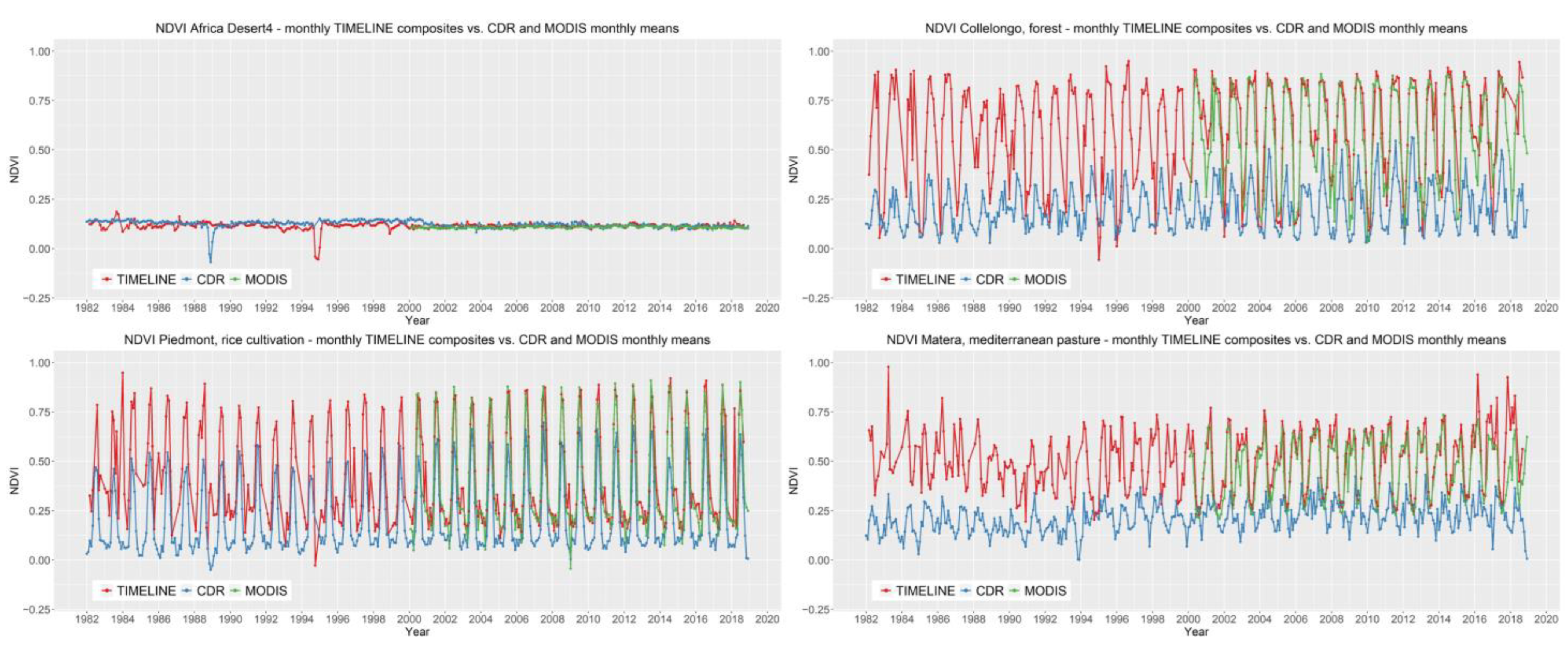
5. Final TIMELINE NDVI Product and Comparison to MODIS and NOAA CDR NDVI

Based on the above described evaluation criteria, the MED approach was selected as best-performing compositing algorithm considering all investigated aspects (Section 4). The final TIMELINE L3 NDVI product currently ranges from 1981–2018 and consists of the daily, decadal, and monthly composites. Each L3 NDVI product consists of a netCDF file with an exhaustive metadata library and six layers: (i) the NDVI for the composite period derived according to the MED compositing; (ii–iii) the Julian day and time of acquisition of the selected observation; and (iv–vi) layers that enable the user to further evaluate the reliability of each NDVI value, namely, a quality layer with bit-encoded information on atmospheric correction and angular information, a layer with the variance of all suitable NDVI values, and a layer with the number of available observations. See Table S3 for a detailed layer description. In addition, a “quicklook” image is provided for each tile.

To evaluate the validity of the selected compositing procedure for the entire production period, the TIMELINE NDVI time series was plotted with the MODIS NDVI product as well as with the NOAA CDR time series at the 37 stations. The NOAA CDR NDVI is produced for the entire lifetime of the NOAA missions. However, it is only available as a daily data set and was aggregated to monthly intervals through calculating the monthly mean for enabling a direct comparison to MODIS and the TIMELINE product. The MODIS product is directly comparable to our monthly composites, but it has only been available since 2000.

For visualization of the results, plots from four different land-cover classes have been selected (Figure 11). The top left figure shows the “Africa Desert4” desert site (site #1 in Figure 1). All three NDVI products agree well with stable NDVI values around 0.125. This high conformity over a stable desert site is in agreement with previous studies [116]. Outliers are clearly visible in this time series, which occur infrequently in the TIMELINE (red spikes) and CDR (blue spikes) time series. Only the MODIS time series is not affected by outliers. At the forest site “Collelongo” (top right in Figure 11) in Central Italy (site #17), however, larger differences between the NDVI products become apparent. While in the TIMELINE time series the yearly phenological cycle of this broadleaf forest compasses the entire plausible NDVI range between 0 and 1, the amplitude of the CDR product is much smaller, hardly reaching NDVI values of 0.5, especially in the early years. It seems that the timing of green-up and senescence is similar in both data sets, with the TIMELINE time series rising a bit earlier and falling a bit later than CDR. Despite the fact that the comparison to MODIS is restricted to the years 2000–2018, it is evident that the absolute values and amplitudes of the MODIS and TIMELINE NDVI agree much better with each other than with the CDR product. The seasonal cycles overlap very well; however, NDVI reduction during senescence occurs a bit later in the TIMELINE than in the MODIS data set.

These observations are valid for the most part also when looking at the agricultural “Piedmont” site (bottom left in Figure 11, site #12). While the difference in amplitude between TIMELINE and CDR is not as large as for the forest site, TIMELINE NDVI is still significantly higher than the CDR NDVI. Similarly, the agreement with MODIS NDVI on this site is very high with regard to the temporal patterns and the absolute NDVI values, also when looking at the summer and winter minimum and maximum values. On the Mediterranean grassland site “Matera” (bottom right in Figure 11, site #5) the TIMELINE NDVI time series is less stable. This is mainly caused by more outliers occurring on this site, e.g., in 1983, 2016, or 2017, as well as by a phase of low NDVI values in the late 1980s and early 1990s, which is not reflected in the CDR data set. The match to the MODIS time series is however again very close, with the timings of green-up and senescence being in good agreement, apart from the above-mentioned outliers and the mismatch of the NDVIs maximum values in some years.

The large difference between the TIMELINE NDVI and the CDR NDVI makes the comparison of these two NDVI time series difficult, especially when evaluating similarities in phenology and temporal trends. The difference in spatial resolution, with CDR covering 0.05° × 0.05° grid cells while the TIMELINE NDVI has a spatial resolution of 1 km, could be one reason for this offset. Apart from that, differences in the way that tropospheric aerosols are treated during preprocessing could play a role, since these could significantly reduce the NDVI [109]. Nevertheless, this analysis demonstrates in general a good agreement of the TIMELINE NDVI time series with existing products, especially the MODIS time series. It does not show any overarching artificial patterns, trends, or irregularities over time, which indicates that the selected compositing procedure is valid for the entire NOAA AVHRR lifetime.

6. Conclusions

Remote sensing image compositing enables the generation of gap-free, equidistant, and spatially comprehensive time series. Since such data sets are crucial for a wide range of remote sensing applications, especially when targeting large areas, which have to be analyzed in a systematic manner, developing and evaluating compositing techniques is highly relevant. The method comparison conducted in this study assessed different compositing criteria and weighing approaches for daily, decadal, and monthly AVHRR image composites, with the aim to generate a spatially and temporally consistent NDVI time series.

It can be derived that algorithms considering only the viewing and illumination conditions tend to introduce strong geometric artefacts into the NDVI maps (e.g., at image swath borders). Similarly, the uncertainty information available for the used SDR product was not a sufficient selection criterion by its own and produced unstable results. On the other hand, approaches that rely purely or by at least 50% on the NDVI (as, e.g., the MVC), often lead to the NDVI overestimation and saturated pixels. The MED approach proved to be an exception from that rule due to its immanent balancing effect and robustness against geometric artefacts. In consequence, the MED approach was chosen as the best-performing compositing algorithm considering all the investigated aspects. The generated, currently almost 40 years long, TIMELINE NDVI time series showed a consistent behavior and a close agreement to the standard MODIS NDVI product, which potentially enables a smooth integration of both data sets.

However, also the combination of the NDVI value and geometry conditions as selection criteria for the NDVI map composition proved to be a promising approach (see the AN variant) that could be further refined in the future. Future work could therefore focus on an improved quality filtering of the input data, on finetuning of the scores assigned to the acquisition angles and NDVI, respectively, and—most importantly—on the extension of the assessment to further years.

The conducted analyses demonstrate the tremendous influence of a compositing procedure on the resulting composites, especially when longer compositing intervals are envisaged. Furthermore, it was shown that several criteria, i.e., at least spatial and temporal consistency, should be assessed when evaluating compositing methods, since data errors such as the geometric artefacts or a volatile time series might go undetected when looking only at single evaluation measures. Due to the demonstrated high influence of the compositing procedure on the quality of an NDVI time series, it can be assumed to also strongly affect higher level products derived thereof, such as land-cover classifications, change detections, or trend analysis. Compositing methods should therefore be thoroughly tested and the potential limitations of temporal composites should be considered for further analyses.

References

1. Piao, S.; Wang, X.; Park, T.; Chen, C.; Lian, X.; He, Y.; Bjerke, J.W.; Chen, A.; Ciais, P.; Tømmervik, H.; et al. Characteristics, drivers and feedbacks of global greening. Nat. Rev. Earth Environ. 2020, 1, 14–27. [Google Scholar] [CrossRef] [Green Version]
2. Alkama, R.; Cescatti, A. Biophysical climate impacts of recent changes in global forest cover. Science 2016, 351, 600–604. [Google Scholar] [CrossRef] [Green Version]
3. Huang, K.; Xia, J.; Wang, Y.; Ahlström, A.; Chen, J.; Cook, R.B.; Cui, E.; Fang, Y.; Fisher, J.B.; Huntzinger, D.N.; et al. Enhanced peak growth of global vegetation and its key mechanisms. Nat. Ecol. Evol. 2018, 2, 1897–1905. [Google Scholar] [CrossRef]
4. Gu, H.; Qiao, Y.; Xi, Z.; Rossi, S.; Smith, N.G.; Liu, J.; Chen, L. Warming-induced increase in carbon uptake is linked to earlier spring phenology in temperate and boreal forests. Nat. Commun. 2022, 13, 3698. [Google Scholar] [CrossRef] [PubMed]
5. Peñuelas, J.; Rutishauser, T.; Filella, I. Phenology Feedbacks on Climate Change. Science 2009, 324, 887–888. [Google Scholar] [CrossRef] [Green Version]
6. Richardson, A.D.; Keenan, T.F.; Migliavacca, M.; Ryu, Y.; Sonnentag, O.; Toomey, M. Climate change, phenology, and phenological control of vegetation feedbacks to the climate system. Agric. For. Meteorol. 2013, 169, 156–173. [Google Scholar] [CrossRef]
7. Mooney, H.; Larigauderie, A.; Cesario, M.; Elmquist, T.; Hoegh-Guldberg, O.; Lavorel, S.; Mace, G.M.; Palmer, M.; Scholes, R.; Yahara, T. Biodiversity, climate change, and ecosystem services. Curr. Opin. Environ. Sustain. 2009, 1, 46–54. [Google Scholar] [CrossRef]
8. Tang, J.; Körner, C.; Muraoka, H.; Piao, S.; Shen, M.; Thackeray, S.J.; Yang, X. Emerging opportunities and challenges in phenology: A review. Ecosphere 2016, 7, e01436. [Google Scholar] [CrossRef] [Green Version]
9. Kuenzer, C.; Dech, S.; Wagner, W. Remote Sensing Time Series Revealing Land Surface Dynamics: Status Quo and the Pathway Ahead. In Remote Sensing Time Series: Revealing Land Surface Dynamics; Kuenzer, C., Dech, S., Wagner, W., Eds.; Springer International Publishing: Cham, Switzerland, 2015; pp. 1–24. [Google Scholar] [CrossRef]
10. Yang, J.; Gong, P.; Fu, R.; Zhang, M.; Chen, J.; Liang, S.; Xu, B.; Shi, J.; Dickinson, R. The role of satellite remote sensing in climate change studies. Nat. Clim. Chang. 2013, 3, 875–883. [Google Scholar] [CrossRef]
11. Ehrlich, D.; Estes, J.E.; Singh, A. Applications of NOAA-AVHRR 1 km data for environmental monitoring. Int. J. Remote Sens. 1994, 15, 145–161. [Google Scholar] [CrossRef]
12. Dech, S.; Holzwarth, S.; Asam, S.; Andresen, T.; Bachmann, M.; Boettcher, M.; Dietz, A.; Eisfelder, C.; Frey, C.; Gesell, G.; et al. Potential and Challenges of Harmonizing 40 Years of AVHRR Data: The TIMELINE Experience. Remote Sens. 2021, 13, 3618. [Google Scholar] [CrossRef]
13. Holzwarth, S. TIMELINE DLR Website. Available online: www.timeline.dlr.de (accessed on 2 August 2022).
14. Huang, S.; Tang, L.; Hupy, J.P.; Wang, Y.; Shao, G. A commentary review on the use of normalized difference vegetation index (NDVI) in the era of popular remote sensing. J. For. Res. 2021, 32, 1–6. [Google Scholar] [CrossRef]
15. Zeng, Y.; Hao, D.; Huete, A.; Dechant, B.; Berry, J.; Chen, J.M.; Joiner, J.; Frankenberg, C.; Bond-Lamberty, B.; Ryu, Y.; et al. Optical vegetation indices for monitoring terrestrial ecosystems globally. Nat. Rev. Earth Environ. 2022, 3, 477–493. [Google Scholar] [CrossRef]
16. Rouse, J.W.; Haas, R.H.; Schell, J.A.; Deering, D.W. Monitoring vegetation systems in the great plains with ERTS. In Proceedings of the Third Symposium on Significant Results Obtained with ERTS-1; NASA SP-351; pp. 309–317. Available online: https://ntrs.nasa.gov/citations/19740022614 (accessed on 12 March 2023).
17. Huete, A.R. A soil-adjusted vegetation index (SAVI). Remote Sens. Environ. 1988, 25, 295–309. [Google Scholar] [CrossRef]
18. Tucker, C.J.; Townshend, J.R.G.; Goff, T.E. African Land-Cover Classification Using Satellite Data. Science 1985, 227, 369–375. [Google Scholar] [CrossRef]
19. Myneni, R.B.; Keeling, C.D.; Tucker, C.J.; Asrar, G.; Nemani, R.R. Increased plant growth in the northern high latitudes from 1981 to 1991. Nature 1997, 386, 698–702. [Google Scholar] [CrossRef]
20. Mueller, T.; Dressler, G.; Tucker, C.J.; Pinzon, J.E.; Leimgruber, P.; Dubayah, R.O.; Hurtt, G.C.; Böhning-Gaese, K.; Fagan, W.F. Human Land-Use Practices Lead to Global Long-Term Increases in Photosynthetic Capacity. Remote Sens. 2014, 6, 5717–5731. [Google Scholar] [CrossRef] [Green Version]
21. Fensholt, R.; Rasmussen, K.; Kaspersen, P.; Huber, S.; Horion, S.; Swinnen, E. Assessing Land Degradation/Recovery in the African Sahel from Long-Term Earth Observation Based Primary Productivity and Precipitation Relationships. Remote Sens. 2013, 5, 664–686. [Google Scholar] [CrossRef] [Green Version]
22. Atzberger, C.; Klisch, A.; Mattiuzzi, M.; Vuolo, F. Phenological Metrics Derived over the European Continent from NDVI3g Data and MODIS Time Series. Remote Sens. 2014, 6, 257–284. [Google Scholar] [CrossRef] [Green Version]
23. Wang, J.; Dong, J.; Liu, J.; Huang, M.; Li, G.; Running, S.W.; Smith, W.K.; Harris, W.; Saigusa, N.; Kondo, H.; et al. Comparison of Gross Primary Productivity Derived from GIMMS NDVI3g, GIMMS, and MODIS in Southeast Asia. Remote Sens. 2014, 6, 2108–2133. [Google Scholar] [CrossRef] [Green Version]
24. Dardel, C.; Kergoat, L.; Hiernaux, P.; Grippa, M.; Mougin, E.; Ciais, P.; Nguyen, C.-C. Rain-Use-Efficiency: What it Tells us about the Conflicting Sahel Greening and Sahelian Paradox. Remote Sens. 2014, 6, 3446–3474. [Google Scholar] [CrossRef] [Green Version]
25. Stöckli, R.; Vidale, P.L. European plant phenology and climate as seen in a 20-year AVHRR land-surface parameter dataset. Int. J. Remote Sens. 2004, 25, 3303–3330. [Google Scholar] [CrossRef]
26. Potter, C.S.; Klooster, S.; Brooks, V. Interannual Variability in Terrestrial Net Primary Production: Exploration of Trends and Controls on Regional to Global Scales. Ecosystems 1999, 2, 36–48. [Google Scholar] [CrossRef]
27. Pedelty, J.; Devadiga, S.; Masuoka, E.; Brown, M.; Pinzon, J.; Tucker, C.; Vermote, E.; Prince, S.; Nagol, J.; Justice, C.; et al. Generating a Long-term Land Data Record from the AVHRR and MODIS Instruments. In Proceedings of the 2007 IEEE International Geoscience and Remote Sensing Symposium, Barcelona, Spain, 23–28 July 2007; pp. 1021–1025. [Google Scholar]
28. Vermote, E.; NOAA CDR Program. NOAA Climate Data Record (CDR) of AVHRR Normalized Difference Vegetation Index (NDVI), Version 5; NOAA National Centers for Environmental Information: Washington, DC, USA, 2019. [CrossRef]
29. Tucker, C.J.; Pinzon, J.E.; Brown, M.E.; Slayback, D.A.; Pak, E.W.; Mahoney, R.; Vermote, E.F.; El Saleous, N. An extended AVHRR 8-km NDVI dataset compatible with MODIS and SPOT vegetation NDVI data. Int. J. Remote Sens. 2005, 26, 4485–4498. [Google Scholar] [CrossRef]
30. Pinzon, J.E.; Tucker, C.J. A Non-Stationary 1981–2012 AVHRR NDVI3g Time Series. Remote Sens. 2014, 6, 6929–6960. [Google Scholar] [CrossRef] [Green Version]
31. LSA SAF. Normalized Difference Vegetation Index CDR Release 2—Metop; EUMETSAT SAF on Land Surface Analysis; 2021; Available online: https://navigator.eumetsat.int/product/EO:EUM:DAT:0385 (accessed on 12 March 2023).
32. Trigo, I.F.; DaCamara, C.C.; Viterbo, P.; Roujean, J.-L.; Olesen, F.; Barroso, C.; Camacho-de Coca, F.; Carrer, D.; Freitas, S.C.; Garcí-a-Haro, J.; et al. The Satellite Application Facility on Land Surface Analysis. Int. J. Remote Sens. 2011, 32, 2725–2744. [Google Scholar] [CrossRef]
33. Government of Canada. Corrected representation of the NDVI using historical AVHRR satellite images (1 km resolution) from 1987 to 2021. In Statistics Canada; Government of Canada: Ottawa, ON, Canada, 2021. [Google Scholar]
34. Earth Resources Observation and Science (EROS) Center. USGS EROS Archive—AVHRR Normalized Difference Vegetation Index (NDVI) Composites. 2018. Available online: https://www.usgs.gov/centers/eros/science/usgs-eros-archive-avhrr-normalized-difference-vegetation-index-ndvi-composites?qt-science_center_objects=0#qt-science_center_objects (accessed on 12 March 2023).
35. Holben, B.N. Characteristics of maximum-value composite images from temporal AVHRR data. Int. J. Remote Sens. 1986, 7, 1417–1434. [Google Scholar] [CrossRef]
36. Griffiths, P.; Nendel, C.; Hostert, P. Intra-annual reflectance composites from Sentinel-2 and Landsat for national-scale crop and land cover mapping. Remote Sens. Environ. 2019, 220, 135–151. [Google Scholar] [CrossRef]
37. Zhang, Y.; Song, C.; Band, L.E.; Sun, G.; Li, J. Reanalysis of global terrestrial vegetation trends from MODIS products: Browning or greening? Remote Sens. Environ. 2017, 191, 145–155. [Google Scholar] [CrossRef] [Green Version]
38. Cihlar, J.; Manak, D.; D’ Iorio, M. Evaluation of compositing algorithms for AVHRR data over land. IEEE Trans. Geosci. Remote Sens 1994, 32, 427–437. [Google Scholar] [CrossRef]
39. Roy, D.P. Investigation of the maximum Normalized Difference Vegetation Index (NDVI) and the maximum surface temperature (Ts) AVHRR compositing procedures for the extraction of NDVI and Ts over forest. Int. J. Remote Sens. 1997, 18, 2383–2401. [Google Scholar] [CrossRef]
40. Choudhury, B.J.; Digirolamo, N.E.; Dorman, T.J. A comparison of reflectances and vegetation indices from three methods of compositing the AVHRR-GAC data over Northern Africa. Remote Sens. Rev. 1994, 10, 245–263. [Google Scholar] [CrossRef]
41. Qiu, S.; Zhu, Z.; Olofsson, P.; Woodcock, C.E.; Jin, S. Evaluation of Landsat image compositing algorithms. Remote Sens. Environ. 2023, 285, 113375. [Google Scholar] [CrossRef]
42. Wang, L.; Xiao, P.; Feng, X.; Li, H.; Zhang, W.; Lin, J. Effective Compositing Method to Produce Cloud-Free AVHRR Image. IEEE GRSL 2014, 11, 328–332. [Google Scholar] [CrossRef]
43. Chuvieco, E.; Ventura, G.; Martín, M.P. AVHRR multitemporal compositing techniques for burned land mapping. Int. J. Remote Sens. 2005, 26, 1013–1018. [Google Scholar] [CrossRef]
44. Potapov, P.V.; Turubanova, S.A.; Hansen, M.C.; Adusei, B.; Broich, M.; Altstatt, A.; Mane, L.; Justice, C.O. Quantifying forest cover loss in Democratic Republic of the Congo, 2000–2010, with Landsat ETM+ data. Remote Sens. Environ. 2012, 122, 106–116. [Google Scholar] [CrossRef]
45. Roberts, D.; Mueller, N.; Mcintyre, A. High-Dimensional Pixel Composites From Earth Observation Time Series. IEEE Trans. Geosci. Remote Sens. 2017, 55, 6254–6264. [Google Scholar] [CrossRef]
46. Flood, N. Seasonal Composite Landsat TM/ETM+ Images Using the Medoid (a Multi-Dimensional Median). Remote Sens. 2013, 5, 6481–6500. [Google Scholar] [CrossRef] [Green Version]
47. Huete, A.; Didan, K.; Miura, T.; Rodriguez, E.P.; Gao, X.; Ferreira, L.G. Overview of the radiometric and biophysical performance of the MODIS vegetation indices. Remote Sens. Environ. 2002, 83, 195–213. [Google Scholar] [CrossRef]
48. Wolfe, R.E.; Roy, D.P.; Vermote, E. MODIS land data storage, gridding, and compositing methodology: Level 2 grid. IEEE Trans. Geosci. Remote Sens. 1998, 36, 1324–1338. [Google Scholar] [CrossRef] [Green Version]
49. Didan, K.; Munoz, A.B.; Solano, R.; Huete, A. MODIS Vegetation Index User’s Guide (MOD13 Series), Version 3.00, June 2015 (Collection 6); Vegetation Index and Phenology Lab, The University of Arizona: Tucson, AZ, USA, 2015. [Google Scholar]
50. Pinzon, J.E.; Brown, M.E.; Tucker, C.J. EMD Correction of orbital drift artifacts in satellite data stream. In Hilbert-Huang Transform and Its Applications; World Scientific Publishing Co. Pte. Ltd.: Singapore, 2005; pp. 167–186. [Google Scholar] [CrossRef]
51. Swinnen, E.; Veroustraete, F. Extending the SPOT-VEGETATION NDVI Time Series (1998–2006) Back in Time With NOAA-AVHRR Data (1985–1998) for Southern Africa. IEEE Trans. Geosci. Remote Sens. 2008, 46, 558–572. [Google Scholar] [CrossRef]
52. Matsuoka, M.; Kajiwara, K.; Hashimoto, T.; Honda, Y. Composite Method over Land for NOAA/AVHRR GAC Global Data Set. J. Jpn. Soc. Photogramm. Remote Sens. 2001, 40, 6–14. [Google Scholar] [CrossRef]
53. Roy, D.P.; Ju, J.; Kline, K.; Scaramuzza, P.L.; Kovalskyy, V.; Hansen, M.; Loveland, T.R.; Vermote, E.; Zhang, C. Web-enabled Landsat Data (WELD): Landsat ETM+ composited mosaics of the conterminous United States. Remote Sens. Environ. 2010, 114, 35–49. [Google Scholar] [CrossRef]
54. White, J.C.; Wulder, M.A.; Hobart, G.W.; Luther, J.E.; Hermosilla, T.; Griffiths, P.; Coops, N.C.; Hall, R.J.; Hostert, P.; Dyk, A.; et al. Pixel-Based Image Compositing for Large-Area Dense Time Series Applications and Science. Can. J. Remote Sens. 2014, 40, 192–212. [Google Scholar] [CrossRef] [Green Version]
55. Griffiths, P.; van der Linden, S.; Kuemmerle, T.; Hostert, P. A Pixel-Based Landsat Compositing Algorithm for Large Area Land Cover Mapping. IEEE J. Sel. Top. Appl. Earth Obs. Remote Sens. 2013, 6, 2088–2101. [Google Scholar] [CrossRef]
56. Frantz, D.; Röder, A.; Stellmes, M.; Hill, J. Phenology-adaptive pixel-based compositing using optical earth observation imagery. Remote Sens. Environ. 2017, 190, 331–347. [Google Scholar] [CrossRef] [Green Version]
57. Latifovic, R.; Trishchenko, A.P.; Chen, J.; Park, W.B.; Khlopenkov, K.V.; Fernandes, R.; Pouliot, D.; Ungureanu, C.; Luo, Y.; Wang, S.; et al. Generating historical AVHRR 1 km baseline satellite data records over Canada suitable for climate change studies. Can. J. Remote Sens. 2005, 31, 324–346. [Google Scholar] [CrossRef] [Green Version]
58. Vancutsem, C.; Pekel, J.F.; Bogaert, P.; Defourny, P. Mean Compositing, an alternative strategy for producing temporal syntheses. Concepts and performance assessment for SPOT VEGETATION time series. Int. J. Remote Sens. 2007, 28, 5123–5141. [Google Scholar] [CrossRef]
59. Rogge, D.; Bauer, A.; Zeidler, J.; Mueller, A.; Esch, T.; Heiden, U. Building an exposed soil composite processor (SCMaP) for mapping spatial and temporal characteristics of soils with Landsat imagery (1984–2014). Remote Sens. Environ. 2018, 205, 1–17. [Google Scholar] [CrossRef] [Green Version]
60. Hagolle, O.; Morin, D.; Kadiri, M. Detailed Processing Model for the Weighted Average Synthesis Processor (WASP) for Sentinel-2 (1.4). 2018. Available online: https://zenodo.org/record/1401360 (accessed on 12 March 2023).
61. Zhu, Z.; Woodcock, C.E.; Holden, C.; Yang, Z. Generating synthetic Landsat images based on all available Landsat data: Predicting Landsat surface reflectance at any given time. Remote Sens. Environ. 2015, 162, 67–83. [Google Scholar] [CrossRef]
62. Vuolo, F.; Ng, W.-T.; Atzberger, C. Smoothing and gap-filling of high resolution multi-spectral time series: Example of Landsat data. Int. J. Appl. Earth. Obs. Geoinf. 2017, 57, 202–213. [Google Scholar] [CrossRef]
63. Chen, P.Y.; Srinivasan, R.; Fedosejevs, G.; Kiniry, J.R. Evaluating different NDVI composite techniques using NOAA-14 AVHRR data. Int. J. Remote Sens. 2003, 24, 3403–3412. [Google Scholar] [CrossRef]
64. Bicheron, P.; Leroy, M. Bidirectional reflectance distribution function signatures of major biomes observed from space. J. Geophys. Res. 2000, 105, 26669–26681. [Google Scholar] [CrossRef]
65. Roy, D.P.; Lewis, P.; Schaaf, C.; Devadiga, S.; Boschetti, L. The Global Impact of Clouds on the Production of MODIS Bidirectional Reflectance Model-Based Composites for Terrestrial Monitoring. IEEE GRSL 2006, 3, 452–456. [Google Scholar] [CrossRef] [Green Version]
66. Gao, F.; Jin, Y.; Schaaf, C.B.; Strahler, A.H. Bidirectional NDVI and atmospherically resistant BRDF inversion for vegetation canopy. IEEE Trans. Geosci. Remote Sens. 2002, 40, 1269–1278. [Google Scholar] [CrossRef]
67. Goward, S.N.; Markham, B.; Dye, D.G.; Dulaney, W.; Yang, J. Normalized difference vegetation index measurements from the advanced very high resolution radiometer. Remote Sens. Environ. 1991, 35, 257–277. [Google Scholar] [CrossRef]
68. Steven, M.D.; Malthus, T.J.; Baret, F.; Xu, H.; Chopping, M.J. Intercalibration of vegetation indices from different sensor systems. Remote Sens. Environ. 2003, 88, 412–422. [Google Scholar] [CrossRef]
69. Bachmann, M.; Tungalagsaikhan, P.; Ruppert, T.; Dech, S. Calibration and Pre-processing of a Multi-decadal AVHRR Time Series. In Remote Sensing Time Series: Revealing Land Surface Dynamics; Kuenzer, C., Dech, S., Wagner, W., Eds.; Springer International Publishing: Cham, Switzerland, 2015; pp. 43–74. [Google Scholar] [CrossRef]
70. Ji, L.; Brown, J.F. Effect of NOAA satellite orbital drift on AVHRR-derived phenological metrics. Int. J. Appl. Earth. Obs. Geoinf. 2017, 62, 215–223. [Google Scholar] [CrossRef]
71. McGregor, J.; Gorman, A.J. Some considerations for using AVHRR data in climatological studies: I. Orbital characteristics of NOAA satellites. Int. J. Remote Sens. 1994, 15, 537–548. [Google Scholar] [CrossRef]
72. Gutman, G.; Masek, J.G. Long-term time series of the Earth’s land-surface observations from space. Int. J. Remote Sens. 2012, 33, 4700–4719. [Google Scholar] [CrossRef]
73. Kern, A.; Marjanović, H.; Barcza, Z. Evaluation of the Quality of NDVI3g Dataset against Collection 6 MODIS NDVI in Central Europe between 2000 and 2013. Remote Sens. 2016, 8, 955. [Google Scholar] [CrossRef] [Green Version]
74. Fensholt, R.; Proud, S.R. Evaluation of Earth Observation based global long term vegetation trends—Comparing GIMMS and MODIS global NDVI time series. Remote Sens. Environ. 2012, 119, 131–147. [Google Scholar] [CrossRef]
75. Peel, M.C.; Finlayson, B.L.; McMahon, T.A. Updated world map of the Köppen-Geiger climate classification. Hydrol. Earth Syst. Sci. 2007, 11, 1633–1644. [Google Scholar] [CrossRef] [Green Version]
76. Bohn, U.; Zazanashvili, N.; Nakhutsrishvili, G.; Ketskhoveli, N. The Map of the Natural Vegetation of Europe and its application in the Caucasus Ecoregion. Bull. Georgian Natl. Acad. Sci. 2007, 175, 112–121. [Google Scholar]
77. ICOS. Standardised Greenhouse Gas Measurements throughout Europe. Available online: https://www.icos-cp.eu/ (accessed on 20 January 2023).
78. Pisek, J.; Erb, A.; Korhonen, L.; Biermann, T.; Carrara, A.; Cremonese, E.; Cuntz, M.; Fares, S.; Gerosa, G.; Grünwald, T.; et al. Retrieval and validation of forest background reflectivity from daily Moderate Resolution Imaging Spectroradiometer (MODIS) bidirectional reflectance distribution function (BRDF) data across European forests. Biogeosciences 2021, 18, 621–635. [Google Scholar] [CrossRef]
79. CEOS Cal/Val Portal. PICS: Pseudo-Invariant Calibration Sites. Available online: https://calvalportal.ceos.org/pics_sites (accessed on 20 January 2023).
80. CEOS Cal/Val Portal. LANDNET SITES (CEOS Reference Sites). Available online: https://calvalportal.ceos.org/ceos-landnet-sites (accessed on 20 January 2023).
81. GHG Europe Database. GHG Europe Database. Available online: http://gaia.agraria.unitus.it/ghg-europe (accessed on 20 January 2023).
82. National Physical Laboratory, U.o.S.; EOLab. Fiducial Reference Measurements for Vegetation. Available online: https://frm4veg.org/ (accessed on 20 January 2023).
83. Forschungszentrum Jülich. TERENO Northeastern Lowland Observatory Test Sites. Available online: https://www.tereno.net/joomla/index.php/observatories/northeast-german-lowland-observatory/test-sites (accessed on 20 January 2023).
84. Davidson, A. Joint Experiment for Crop Assessment and Monitoring (JECAM), Germany-DEMMIN. Available online: http://jecam.org/studysite/germany-demmin/ (accessed on 20 January 2023).
85. Koslowsky, D. Mehrjährige Validierte und Homogenisierte Reihen des Reflexionsgrades und des Vegetationsindexes von Landoberflächen aus Täglichen AVHRR-Daten Hoher Auflösung. Ph.D. Thesis, Freie Universität Berlin, Berlin, Germany, 1996. [Google Scholar]
86. Defourny, P.; Kirches, G.; Militzer, J.; Boettcher, M.; Brockmann, C.; Bontemps, S. Land Cover CCI Product ValidationAnd Intercomparison Report v2; UCL-Geomatics: Louvain-la-Neuve, Belgium, 2017; p. 374. [Google Scholar]
87. Cuntz, M.; Aiguier, T.; Courtois, P.; Joetzjer, E.; Lily, J. Hesse ICOS Station. Available online: https://meta.icos-cp.eu/resources/stations/ES_FR-Hes (accessed on 20 January 2023).
88. Kidwell, K.B. NOAA Polar Orbiter Data Users Guide: (TIROS-N, NOAA-6, NOAA-7, NOAA-8, NOAA-9, NOAA-10, NOAA-11, NOAA-12, NOAA-13, and NOAA-14); National Oceanic and Atmospheric Administration, and National Climatic Data Center (U.S.), Satellite Data Services Division: Washington, DC, USA, 1995.
89. Robel, J.; Graumann, A. NOAA KLM User’s Guide with NOAA-N, N Prime, and MetOp Supplements; National Oceanic and Atmospheric Administration, National Environmental Satellite, Data, and Information Service National Climatic Data Center, Remote Sensing and Applications Division: Washington, DC, USA, 2014.
90. Molch, K.; Leone, R.; Frey, C.; Wolfmüller, M.; Tungalagsaikhan, P. NOAA AVHRR Data Curation and Reprocessing—TIMELINE. In Proceedings of the Big Data from Space (BiDS’ 2013), Frascati, Italy, 5–7 June 2013. [Google Scholar]
91. Trishchenko, A.P. Effects of spectral response function on surface reflectance and NDVI measured with moderate resolution satellite sensors: Extension to AVHRR NOAA-17, 18 and METOP-A. Remote Sens. Environ. 2009, 113, 335–341. [Google Scholar] [CrossRef]
92. Molling, C.C.; Heidinger, A.K.; Straka, W.C.; Wu, X. Calibrations for AVHRR channels 1 and 2: Review and path towards consensus. Int. J. Remote Sens. 2010, 31, 6519–6540. [Google Scholar] [CrossRef]
93. Santamaria-Artigas, A.; Vermote, E.F.; Franch, B.; Roger, J.-C.; Skakun, S. Evaluation of the AVHRR surface reflectance long term data record between 1984 and 2011. Int. J. Appl. Earth. Obs. Geoinf. 2021, 98, 102317. [Google Scholar] [CrossRef]
94. Dietz, A.J.; Frey, C.M.; Ruppert, T.; Bachmann, M.; Kuenzer, C.; Dech, S. Automated Improvement of Geolocation Accuracy in AVHRR Data Using a Two-Step Chip Matching Approach—A Part of the TIMELINE Preprocessor. Remote Sens. 2017, 9, 303. [Google Scholar] [CrossRef] [Green Version]
95. Bachmann, M.; Müller, T. Using spaceborne hyperspectral data for spectral cross-calibration of multispectral sensors. In Proceedings of the 2015 IEEE International Geoscience and Remote Sensing Symposium (IGARSS), Milan, Italy, 26–31 July 2015; pp. 2813–2815. [Google Scholar]
96. Dietz, A.J.; Klein, I.; Gessner, U.; Frey, C.M.; Kuenzer, C.; Dech, S. Detection of Water Bodies from AVHRR Data—A TIMELINE Thematic Processor. Remote Sens. 2017, 9, 57. [Google Scholar] [CrossRef] [Green Version]
97. Kriebel, K.T.; Gesell, G.; Kastner, M.; Mannstein, H. The cloud analysis tool APOLLO: Improvements and validations. Int. J. Remote Sens. 2003, 24, 2389–2408. [Google Scholar] [CrossRef]
98. Kriebel, K.T.; Saunders, R.W.; Gesell, G. Optical Properties of Clouds Derived from Fully Cloudy AVHRR Pixels. Beiträge zur Physik der Atmosphäre 1989, 62, 165–171. [Google Scholar]
99. Saunders, R.W.; Kriebel, K.T. An improved method for detecting clear sky and cloudy radiances from AVHRR data. Int. J. Remote Sens. 1988, 9, 123–150. [Google Scholar] [CrossRef]
100. Klüser, L.; Killius, N.; Gesell, G. APOLLO_NG—A probabilistic interpretation of the APOLLO legacy for AVHRR heritage channels. Atmos. Meas. Tech. 2015, 8, 4155–4170. [Google Scholar] [CrossRef] [Green Version]
101. Berk, A.; Anderson, G.P.; Acharya, P.K.; Shettle, E.P. Modtran® 5.2.0.0 User’s Manual; Air Force Research Laboratory, Space Vehicles Directorate, Air Force Materiel Command Hanscom AFB: Burlington, MA, USA, 2008. [Google Scholar]
102. NASA. About MODIS. Available online: https://modis.gsfc.nasa.gov/about/ (accessed on 15 November 2022).
103. NASA. MODIS Specifications. Available online: https://modis.gsfc.nasa.gov/about/specifications.php (accessed on 15 November 2022).
104. Didan, K. MODIS/Terra Vegetation Indices 16-Day L3 Global 1 km SIN Grid V061 [Data Set]. NASA EOSDIS Land Processes DAAC. Available online: https://lpdaac.usgs.gov/products/mod13a2v061/ (accessed on 15 November 2022).
105. Didan, K. MODIS/Terra Vegetation Indices Monthly L3 Global 1 km SIN Grid V061 [Data Set]. NASA EOSDIS Land Processes DAAC. Available online: https://lpdaac.usgs.gov/products/mod13a3v061/ (accessed on 15 November 2022).
106. Didan, K. Status for: Vegetation Indices (MOD13). Available online: https://modis-land.gsfc.nasa.gov/ValStatus.php?ProductID=MOD13 (accessed on 3 March 2023).
107. Huete, A.; Justice, C.; van Leeuwen, W.J.D.; Jacobson, A.; Solanos, R.; Laing, T.D. MODIS VEGETATION INDEX (MOD 13) Algorithm Theoretucal Basis Document, Version 3; Vegetation Index and Phenology Lab.: Tucson, AZ, USA, 1999. [Google Scholar]
108. NASA; EOSDIS; LAADS; DAAC. Long-Term Data Record. Available online: https://ladsweb.modaps.eosdis.nasa.gov/missions-and-measurements/applications/ltdr/#project-documentation (accessed on 6 March 2023).
109. Vermote, E. AVHRR Surface Reflectance and Normalized Difference Vegetation Index—Climate Algorithm Theoretical Basis Document, NOAA Climate Data Record Program CDRP-ATBD-0459 Revsion 2; NOAA Central Library: Washington, DC, USA, 2018. Available online: https://www.ncei.noaa.gov/pub/data/sds/cdr/CDRs/Normalized_Difference_Vegetation_Index/AVHRR/AlgorithmDescriptionAVHRR_01B-20b.pdf (accessed on 12 March 2023).
110. Cihlar, J.; Ly, H.; Li, Z.; Chen, J.; Pokrant, H.; Huang, F. Multitemporal, multichannel AVHRR data sets for land biosphere studies—Artifacts and corrections. Remote Sens. Environ. 1997, 60, 35–57. [Google Scholar] [CrossRef]
111. Gutman, G.G. Vegetation indices from AVHRR: An update and future prospects. Remote Sens. Environ. 1991, 35, 121–136. [Google Scholar] [CrossRef]
112. Kimes, D.S. Dynamics of directional reflectance factor distributions for vegetation canopies. Appl. Opt. 1983, 22, 1364–1372. [Google Scholar] [CrossRef]
113. Cihlar, J.; Huang, F. Effect of atmospheric correction and viewing angle restriction on AVHRR data composites. Can. J. Remote Sens. 1994, 20, 132–137. [Google Scholar]
114. van Leeuwen, W.J.D.; Huete, A.R.; Laing, T.W. MODIS Vegetation Index Compositing Approach: A Prototype with AVHRR Data. Remote Sens. Environ. 1999, 69, 264–280. [Google Scholar] [CrossRef]
115. Meyer, D.; Verstraete, M.; Pinty, B. The effect of surface anisotropy and viewing geometry on the estimation of NDVI from AVHRR. Remote Sens. Rev. 1995, 12, 3–27. [Google Scholar] [CrossRef]
116. Vermote, E.F.; Saleous, N.Z. Calibration of NOAA16 AVHRR over a desert site using MODIS data. Remote Sens. Environ. 2006, 105, 214–220. [Google Scholar] [CrossRef]
Figure 1. Extent of the TIMELINE study area in LAEA ETRS89-extended projection with L3 tile borders (white), location of the focus areas A–F (see Section 2.4.2, in yellow), and location of the investigated sites (red dots, see Table S1 for site numbers). The background map shows an RGB false color composite (logarithmic stretch) of the three-month mean of monthly (May, June, and July 2007) median red and NIR reflectance composites, with red = band 1 (red reflectance), green = band 2 (NIR reflectance), and blue = band 1. Data gaps (which include inland water bodies) are displayed in white, while oceans are light blue.
Remotesensing 15 01631 g001
Figure 2. TIMELINE Processing chain from L0 raw data to NDVI L3.
Remotesensing 15 01631 g002
Figure 3. Schematic overview on categories of used compositing approaches. The term “Angles” corresponds to a combined weight of all investigated angles, i.e., satellite and sun zenith angles as well as relative azimuth angle, which are all equally weighted.
Remotesensing 15 01631 g003
Figure 4. Violin plots of NDVI (top), satellite zenith (middle), and sun zenith angles (bottom) distributions of each variant, including samples (n = 100,000 per map) from all monthly composites.
Remotesensing 15 01631 g004
Figure 5. Monthly NDVI maps based on the different compositing approaches for May 2007. The MOD13A3 product of the same month is shown for comparison in the lower right tile.
Remotesensing 15 01631 g005aRemotesensing 15 01631 g005b
Figure 6. Deviation of the monthly composites generated with compositing approaches from MODIS NDVI for the entire TIMELINE area.
Remotesensing 15 01631 g006
Figure 7. Zoom to focus A (left column), B (middle column), and C (right column) of the monthly NDVI maps based on the different compositing approaches. For focus area locations, see Figure 1.
Remotesensing 15 01631 g007aRemotesensing 15 01631 g007bRemotesensing 15 01631 g007c
Figure 8. Time series of daily (top), decadal (middle), and monthly (bottom) NDVI at the Algeria 5 (exemplary desert site), Hesse (exemplary forest site), and Piedmont (exemplary agriculture site) stations. In black, the MOD13A2 (16 days interpolated to decadal and daily intervals, respectively, top and middle) and MOD13A3 (monthly, bottom) are plotted as references. For better visualization, graphs are split up, showing the “single variable composites” (MVC, MED, Sa, Su, Az, and Uc) and the “multiple variable composites” (NAUc, AN, SuSaAzUc, AUc, and MOD) separately in Figure S6.
Remotesensing 15 01631 g008
Figure 9. Deviations of monthly composites from MODIS values at 37 stations.
Remotesensing 15 01631 g009
Figure 10. Neighborhood homogeneity characterized by DOY (top), satellite zenith (middle), and sun zenith variance (bottom) in 3 × 3 window of all monthly composites for all variants.
Remotesensing 15 01631 g010
Figure 11. TIMELINE NDVI time series examples at four stations (the desert site “Africa desert 4” (top left); the forest site “Collelongo” (top right), the agricultural site “Piedmont” (bottom left), and the grassland site “Matera” (bottom right)) in comparison to the CDR und MODIS products.
Remotesensing 15 01631 g011