Abstract
Here we investigate properties of ocean eddies in the key Arctic region of the northern Greenland Sea and the Fram Strait using visible and infrared Moderate Resolution Imaging Spectroradiometer (MODIS) Aqua data acquired from April to September in 2007 and 2018–2020. We infer eddy properties using visual identification and automated processing of their signatures in sea surface temperature (SST) and chlorophyll-a (chl-a) maps, and their gradients. Altogether, 450 (721) eddies were identified in SST (chl-a) data. Their radii span from 2 to 40 km (mean value 12 km). Most eddies are elliptical with a mean aspect ratio (eccentricity) of their axes equal 0.77 (0.64). Cyclones are smaller than anticyclones and prevail in both data sources. Cyclones tend to be more prevalent over shallow shelves, and anticyclones over deep water regions. Peak eddy activity is registered in June, while chl-a data also possess a second peak in April. In SST, the highest eddy probability is found along the East Greenland Current in the Nordbukta region at 76–78°N and along the West Spitsbergen Current at 78–80°N. In chl-a, most of them are observed in the central Fram Strait. The overall number of eddies with a positive chl-a anomaly, dominated by cyclones, is larger (62%) than that with a negative one (~38%). The number of eddies with positive and negative SST anomalies is nearly equal. Eddy translation velocities are 0.9–9.6 km/day (mean value 4.2 km/day). Despite frequent cloud and ice cover, MODIS data is a rich source of information on eddy generation hot-spots, their spatial properties, dynamics and associated SST and chl-a anomalies in the Arctic Ocean.
Keywords:
ocean eddies; submesoscale dynamics; MODIS Aqua; SST; chlorophyll-a; Fram Strait; Greenland Sea; Arctic Ocean 1. Introduction
Submesoscale and mesoscale eddies play an important role in the oceanic energy cascade [1,2], water mixing and stirring, heat and substance transfer [3,4,5,6,7], biological enhancement, pelagic fluxes and development of planktonic organisms in the Arctic Ocean (AO) [8,9,10]. Properties of mesoscale eddies and their associated implications have been actively studied in the AO for almost 50 years now using a variety of in situ methods [4,11,12,13,14,15,16,17,18,19,20,21,22,23,24] and numerical models [25,26,27,28,29,30].
Recent field experiments are also successful in revealing the fine structure of nonlinear submesoscale dynamic features [1,3,31]; however, such observations are still rare in the AO. Contemporary high-resolution (~1 km) eddy-resolving models show promising results in resolving submesoscales but, due to relatively small values of the first baroclinic Rossby radius in the AO [32,33], still require very high mesh resolution and sustained supporting observations [2,6,28,34,35].
In turn, satellite remote sensing has proven the ability to effectively observe properties of eddies of various scales both over open ocean and within marginal ice zones [7,34,36,37,38,39,40,41,42] using passive and active sensing techniques. As sea ice declines in the Arctic Ocean, it is expected that the role of remote sensing from satellites and unmanned aerial vehicles would also increase [33,43].
In this work, we analyze the oceanic eddy field in the key Arctic region located between 74° and 82°N in the northern Greenland Sea and the Fram Strait using satellite optical data. The region is the main gateway of water exchange between the Arctic Ocean and the North Atlantic [44,45], characterized by the largest eddy kinetic energy across the entire AO [2,21]. Here, the West Spitsbergen Current (WSC) carrying the warm Atlantic Water (AW) moves northward and meets the cold Polar Water (PW) of the East Greenland Current (EGC) moving southward [26].
The area is known for active eddy generation as a result of the barotropic and baroclinic instabilities of the main boundary currents in the Fram Strait [14,26,27,28,45] and downstream in the Nansen Basin [18,46,47,48], revealed from a large number of moored and shipborne measurements, numerical models and satellite observations.
The latter were primarily based on measurements of active microwaves devices, i.e., spaceborne radars—synthetic aperture radars (SARs) and altimeters [34,37,38,49,50]. Their signal does not depend on illumination conditions and easily penetrates through clouds that are frequent in the Arctic. Analysis of these data enabled the obtaining of solid statistics of eddies, including their key generation sites, spatial and dynamic properties by observing their footprints in sea surface roughness and sea level anomalies at horizontal scales of 1–50 km and 10–100 km, respectively. Such measurements, however, do not provide any means to directly relate the observed eddy features to actual thermal and/or biological structures of the study region, nor assess the eddy-induced modulation of these properties.
To fill this gap and assess the potential of “classical” medium resolution satellite optical data for observing the Arctic eddies, here we use visible and infrared data acquired by Moderate Resolution Imaging Spectroradiometer (MODIS) from April to September in 2007 and 2018–2020. Previously, MODIS data were already exploited to some extent in order to get a spatial view of water dynamics, eddies and eddy-induced ice movement in the Western Arctic Ocean [31,38,41,51]. However, to our knowledge, such data were not used to build a systematic and detailed picture of the eddy field in any Arctic region as is done here.
2. Materials and Methods
In this work we use visible and infrared MODIS data onboard an Aqua satellite to investigate the properties of ocean eddies in the northern Greenland Sea and the Fram Strait bounded by 73°−83°N and 21°W−31°E (Figure 1). We use two types of satellite imagery: sea surface temperature (SST) derived from long-wave (11–12 µm) thermal radiation [52] and the concentration of the photosynthetic pigment chlorophyll-a (chl-a) produced using the OC3 algorithm [53,54]. Both data types are Level-2 datasets provided by the MODIS Aqua instrument. The reprocessing version of SST is 2019.0 [55] and the version of chl-a is 2018.0 [56].
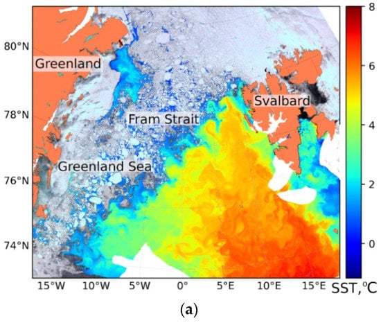
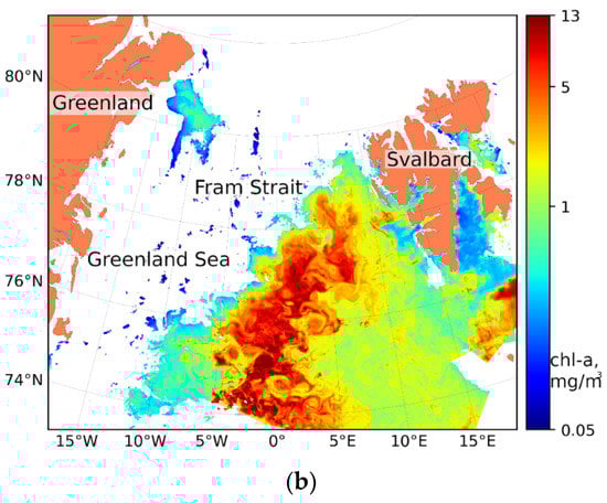
Figure 1.
Example of eddying features in sea ice, SST (a), and chl-a (b) maps of the study region. Sea ice true color image is built from the MODIS image acquired on 14 June 2019, while SST and chl-a data are obtained from MODIS images acquired on 14–16 June 2019. White regions in (b) mask sea ice and clouds.
The data were collected during an extended summer season (from April to October) in 2007 and 2018–2020. As no eddies were identified in October, we did not consider this month in the analysis below. The choice of years is dictated by the intention to capture diversity in sea ice conditions with one of the first ice minima recorded in 2007, comparing it to the recent years of 2018–2020. Moreover, the years of 2007 and 2018 are the years for which an additional information on eddy properties is available from the analysis of in situ, spaceborne SARs, with altimetry and high-resolution model data [7,34,48,49] to be compared in later studies.
We process SST and chl-a data separately but in a similar way. Single swath images are manually browsed and the relatively cloud-free data (with at least 10–20% of cloud-free regions) are selected. For these cloud-free data, all single swath images available during the same day are reprojected to a regular grid and then averaged into daily images. The time span when MODIS Aqua images are acquired covers almost the entire 24 h, apart from a short interval from 5 p.m. to 9 p.m. The average number of satellite overpasses during the day is 11 and 9 for SST and chl-a data, respectively. In this sense, the resulting maps are truly daily-averaged as the images used for the averaging cover very different parts of the day. In this case, one might expect some effects of diurnal variability of SST and chl-a in the resulting daily-averaged maps. However, we presume that this effect is almost negligible, as most of the data are acquired during the polar day when the sun illumination conditions do not change much during the entire 24 h.
The grid is the same for SST and chl-a data with a spatial resolution of 0.5 km along the meridian and not coarser than 0.5 km along the parallel. Additional masking is performed for SST data in order to achieve uniform data coverage for the both data sources, i.e., a much stricter chl-a cloud-ice mask is applied to SST data.
For SST data, 15,138 satellite images are used in total. The number of images amounts to 3857, 4177, 3777 and 3327 images for years 2007, 2018, 2019 and 2020, respectively. For chl-a data, 9902 satellite images are used. The number of images amounts to 2691, 2635, 1976 and 2602 images for years 2007, 2018, 2019 and 2020, respectively. The list of the relatively cloud-free days, identical for SST and chl-a data, subjected to further analysis, amounts to 41, 60, 38, and 31 days for the respective years.
The data availability affects how many eddies could be identified in certain areas during a certain time period. If SST or chl-a image is considered “good” and is subjected to further analysis, it does not mean that the whole swath of the image provides valuable data as a considerable and variable area of the image is often covered by clouds or ice. To account for this variability, the effective data coverage is estimated on a pixel basis as a number of times the pixel contains an ice- and/or cloud-free data in the daily-averaged image (Figure 2). As we consider daily-averaged images then the data coverage could be expressed in days. Initially, a spatial distribution of the data coverage was not similar for SST and chl-a, but, after applying the same cloud-ice mask, the data coverage became identical for the both data sources. Spatial distribution of the data coverage is shown in Figure 2. As seen, the availability of cloud- and ice-free data is highest west of Svalbard where it reaches 70–90 days. In the south, it is about 20–40 days, while it is only about 10 days in the northwestern Greenland Sea which is quasi-permanently covered by fast ice and the wide marginal ice zone [49].
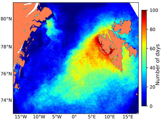
Figure 2.
Coverage of the study region by the cloud- and ice-free SST and chl-a data during the entire study period from April to September in 2007 and 2018–2020.
Data Processing
The identification of eddies is performed over the cloud- and ice-free regions of satellite SST and chl-a daily-averaged maps. The method of satellite data processing, identical for SST and chl-a data, consists of the following consecutive steps: (i) data preparation, (ii) visual identification of eddies and manual extraction of their axes, (iii) automatic identification of various eddy properties. Below we describe each step in more detail.
- (i).
- Based on the daily-averaged SST/chl-a values, horizontal gradients of these properties are calculated using a Sobel operator [57]. The Sobel operator performs a 2-D spatial gradient measurement on an image and so emphasizes regions of high spatial frequency that correspond to edges. The principle involved is that of estimating the gradient of a digitized picture (“density” function or, in our case, SST/chl-a field) at a point by the vector summation of the 4 possible simple central gradient estimates obtained in a 3 × 3 pixel neighborhood. It is a simple and efficient filter that is used to highlight edges and gradients, particularly in the eddy identification process [58,59]. Examples of SST field and corresponding SST gradient with marked eddy axes are presented in Figure 3.
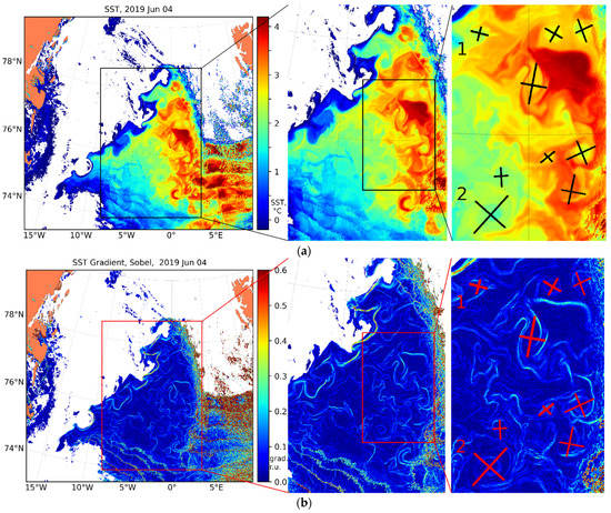 Figure 3. Example of the daily-averaged MODIS SST field (a) and its gradient (b) for 4 June 2019 shown at different scales with zooming made from left to right. Black and red crosses in the rightmost subfigures mark axes of identified eddies. White color shows the regions where clouds and ice are masked.
- (ii).
- Eddies are visually detected and manually identified in the mapped values of the SST/chl-a gradients. The daily-averaged maps of SST/chl-a gradients are viewed until all eddies that are unambiguously visible in the image are identified by drawing the eddy axes. An example of identification of eddies’ axes is given in Figure 3 (see subfigures on the right). In the case of a relatively circular eddy or in the case of eddy with several spiraling maxima, axes are drawn to the outer maxima of gradients. In the case of unclosed gradient lines, the axes are drawn to the maxima of the most closed gradient. During the analysis, mushroom-like pairs of cyclonic and anticyclonic eddies are identified and measured independently as two eddies. In most cases, the eddy is clearly manifested in SST/chl-a gradient field and is easily identified regardless of their absolute values inside the eddy and the water around it. For example, the eddy “2” in Figure 3 is well traced in the SST gradient field, although it is not very clearly visible in the initial SST data. The disadvantage of using gradient fields is their high sensitivity to noise in the data and the artifacts of the data averaging. For example, the eddy “1” in the upper left corner of Figure 3b has artifacts impeding its identification, but in the initial SST field, these artifacts do not appear and the overall eddy structure is easy to identify. Thus, the SST/chl-a gradient fields are used as the main source of information on the position, size and form of eddies, while the initial SST/chl-a fields serve as an auxiliary information. The use of two fields results in more reliable eddy detection in the case of the presence of minor errors in one of them.
It is important to note that a particular eddy that is well visible, e.g., in the chl-a data, is not always visible in the corresponding SST field, and vice versa. The reason for this may be a different number of single swath images available for the creation of the daily-averaged composites that could potentially lead to some data blurring effects and error accumulation. Another source for discrepancies may arise from the different nature of eddy tracers in SST and chl-a fields. The SST field is relatively conservative while the chl-a field, apart from being passively transported, is subjected to variations due to phytoplankton development during vegetational season [60].
Each identified eddy is characterized by major and minor axes and the rotation sign (cyclonic or anticyclonic). Numerically, the eddy axes are defined by four pairs of geographic coordinates defining the ends of each eddy axis. The rotation sign (or eddy polarity) was determined from the visual analysis of the spiral structure of eddies. This is described, e.g., in [61], and can be inferred assuming a developing shear instability of a spiraling eddy when the location of eddy spiral relative to the source region (e.g., “leg” of a mushroom-like vortex) and its rotation direction from the outer edge toward the eddy center allows us to guess the polarity. In the case of absence of spiraling lines or closed gradient lines, the eddy was identified as an eddy with an undefined rotation sign. The number of such eddies was equal to 3.6% for SST and 11.7% for chl-a out of the total number of eddies identified in these data sets.
- (iii).
- Automatic processing of eddies relies on the manually-drawn axes to compute eddy shape, size, location and to analyze eddy influence on the spatial distribution of SST/chl-a. First, an ellipse is drawn at the extreme points of the axes during the automatic post-processing. Second, the coordinates of the eddy center are defined as a geographic point where major and minor axes intersect. The size of the eddy is then determined in terms of minor and major radii averaged into a mean value. The eddy radius is calculated as R = (Amaj/2 + Amin/2)/2, and the aspect ratio (AR) of two axes as AR = Amin/Amaj, where Amaj and Amin are major and minor eddy axes, respectively [62].
To estimate the effect of eddies on SST or chl-a distribution, all eddies are divided into three types. In the first two types, SST or chl-a values in the eddy core are either higher or lower than the background value over the surrounding waters. The latter is defined from the corresponding SST/chl-a values along the continuation of eddy axes extending outside the eddy by half of the eddy axis in each direction (see Figure 4). However, if other eddies are present nearby (e.g., in the case of eddy dipoles), we consider only one axis that did not “touch” the nearby eddy. The third type is assigned to the eddies that do not possess any well-defined single-sign SST/chl-a anomalies compared to the ambient waters. The eddy type (positive, negative or undefined anomaly) is estimated independently for SST and chl-a. Eddies for which the data in the surrounding waters are of bad quality (due to presence of speckles/artifacts in the vicinity of clouds, ice or swath averaging boundaries) or absent are excluded from the analysis.
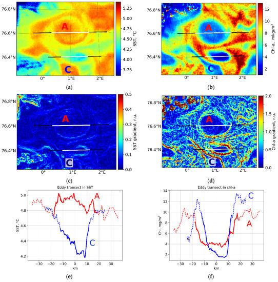
Figure 4.
MODIS Aqua maps of SST (a), chl-a (b), SST gradient (c), and chl-a gradient (d) field of on 15 June 2019 with a distinct manifestation of an eddy dipole. Black and white lines in (a–d) show transects crossing the surrounding waters and the eddies, respectively. Spatial variations of SST (e) and chl-a (f) values along transects crossing anticyclone (red line) and cyclone (blue line). Eddy cores in (e,f) are shown by solid line and the ambient waters—by dashed line.
Figure 4 illustrates an identification of an eddy dipole that is manifested in MODIS Aqua SST and chl-a images acquired on 15 June 2019. The core of its anticyclonic part A is warmer and has a lower chl-a concentration than the water on the periphery and outside of it. In turn, the core of cyclone C has rather pronounced negative SST and chl-a anomalies relative to the ambient water. Boundaries of this dipole are also well seen in the corresponding gradient fields (Figure 4c,d), while the variations of SST/chl-a values along the axes allow us to define eddy-induced anomalies in SST/chl-a fields (Figure 4e,f). In this case, we define that the anticyclone A has positive (yet, rather small) SST and negative chl-a anomalies, while the cyclone C has negative SST and chl-a anomalies.
3. Results
Upon analysis of the data, 450 eddies were identified in SST data: 40, 61, 171 and 147 eddies in April–September of 2007, 2018, 2019 and 2020, respectively. A higher number, 721 eddies, were identified in the chl-a data: 180, 202, 231 and 108 eddies in 2007, 2018, 2019 and 2020, respectively. For all the available SST (chl-a) data, the number of cyclonic eddies (CEs) is 1.57 (1.34) times greater than that of anticyclonic eddies (ACEs). In 2018 and 2019, this difference was rather small (only 4–6%), while in 2007 it was the largest (30–45%).
The description of main eddy parameters identified in SST fields is given in Table 1. Radii of the identified eddies are in the range of 2.1–30.9 km. The year of 2018 stands out with a minimal range of eddy radii, 3.7–24.8 km. The mean eddy radius during the four years is 12 km (Table 1). The eddy AR values do not vary strongly in different years and fluctuate in the range of 0.40–1.00. This range is greater during the years with a larger number of eddies (Table 1, Columns “Min AR”, “Max AR”).

Table 1.
Statistical description of eddies identified in MODIS SST data. N—number of eddies, Nc—number of cyclones, Nac—number of anticyclones, Nu—number of eddies for which the rotation sign was not identified. Nc % and Nac %—percentage of cyclonic and anticyclonic eddies relative to their total number. Min, Max, Mean—minimal, maximal, mean values of eddy radii (R) and their aspect ratio (AR).
The description of main eddy parameters identified in the chl-a data is given in Table 2. A comparison of the results obtained from the two data sources shows certain differences. The overall percentage of cyclones (anticyclones) is smaller (higher) in the chl-a data, but this difference is not statistically significant even at a confidence level of p = 0.1 and may arise due to errors in the eddy detection method, confirming that statistics derived from SST and chl-a datasets describe nearly the same population of eddies. The overall range of the eddy radii is also higher in the chl-a (2.1–30.9 km in SST vs. 2.9–38.9 km in chl-a), while their mean values in both data sources are almost identical. The former could be caused by the higher portion of anticyclones in the chl-a data usually being larger in size than cyclones, as shown below and demonstrated in earlier works [37,50]. A similar comparison for the AR of eddy radii shows that maximum AR for all eddies is 1.0, which is natural, while the minimal values are lower in the chl-a data (0.33) compared to 0.4 in the SST. Their mean values for the both data sources are identical (~0.77).
Table 2.
The same as in Table 1 but for the eddies identified in MODIS chl-a data.
3.1. Seasonal Distribution of Eddies
Seasonal variations in the total number of identified eddies do not have an explicit maximum according to SST data and have a clear maximum in June according to chl-a data (Figure 5a,b). Looking at SST data in more detail shows that the total number of eddies also has a maximum in June; however, this peak is not very pronounced (Figure 5a). Slightly lower but similar values are observed in April and July, while a minimal number of eddies are found in September.
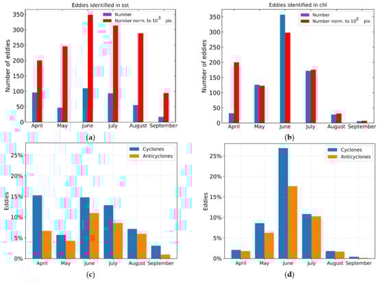
Figure 5.
Monthly distributions of eddies identified in SST (a,c) and chl-a (b,d) data in 2007 and 2018–2020: (a,b) total (blue bars) and the normalized (red bars) numbers of eddies; (c,d) percentage of cyclonic (blue bars) and anticyclonic (orange bars) eddies identified in SST (c) and chl-a data (d).
It is important to note that the monthly data availability is not constant during the study period. It is maximal in June, while in April and September there are six and and-and-a-half times less data than in June, respectively. To account for this fact, and get a more realistic seasonal variation of eddy numbers, a normalization of the data is made by dividing the total number of eddies per month by the number of cloud- and ice-free data available per given month (i.e., the number of such pixels per month).
The SST-based normalized eddy statistics is now better expressed and experiences a gradual increase from April to June followed by a gradual decrease (Figure 5a, red bars). A seasonal variation of the normalized eddy number in the chl-a data is nearly identical to the non-normalized values (Figure 5b) apart of those for April that now become much more expressed. The main peak in the both chl-a statistics is found in June followed by April and July.
Comparing the two normalized data sets, one may see that chl-a data have a more explicit seasonal variation, while the relative changes in SST are not large, especially during June–August. This is potentially linked to the seasonal variations of phytoplankton (and others co-varying optically active components and their depth distribution) concentration, i.e., there could be less phytoplankton and, hence, less tracers to facilitate eddy identification during particular months in spring and autumn. Moreover, seasonal variations in near-surface winds, waves and surface heat flux might be also important and affect the obtained statistics through masking some eddies due to enhanced mixing or intensified cooling/heating.
A relationship between the number of CEs and ACEs does not change much throughout the extended summer period in both data sources (Figure 5c,d). The number of cyclones is always larger than that of anticyclones. However, during most of the period this difference is not large. Nevertheless, during certain months, e.g., in April according to the SST data and in June according to the chl-a data, and in September according to the both data sources, the number of CEs is strongly prevailing over ACEs.
3.2. Locations of Eddies
Spatial distributions of eddies detected in SST and chl-a data are shown in Figure 6. Compared to chl-a, more eddies are identified in SST data over the northwestern shelf of the Greenland Sea and north of 80°N (Figure 6a). In turn, almost no eddies were detected over the Greenland Sea shelf in the chl-a data.
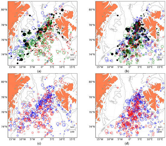
Figure 6.
Spatial distribution of eddies identified in SST (a,c) and in chl-a (b,d) data in 2007 and 2018–2020. Colors in (a,b) specify eddies identified in 2007 (black filled circles), 2018 (blue circles), 2019 (green circles), 2020 (red circles). Colors in (c,d) mark cyclones (blue circles) and anticyclones (red circles). Marker size is proportional to eddy diameter.
Most of them were observed in the Fram Strait and closer to Svalbard, and in the southeastern part of the study region (Figure 6b). A better visibility of eddies in chl-a data in the vicinity of the Spitsbergen west coast could be linked to the higher phytoplankton concentration in coastal waters in June and July (Figure 5b).
The differences between the four studied years are noticeable in both datasets, with 2007 having the least spatial spread and 2018 spreading the most to the north. In 2019 and 2020, the deep-sea area south of 77°N between 5°W and 5°E had a much larger number of eddies in SST than in 2007 and 2018.
Figure 7a,b show spatial maps with a total number of eddies identified per bin on a horizontal grid of 30 × 30 bin with an average bin size of 40 × 40 km. In both data sources, the highest number of eddies (>10 eddies in SST and >20 eddies in chl-a) is found in the central and northeastern parts of the Fram Strait which potentially coincides with the trajectories of the main boundary currents in the region and recirculation branches of the AW.
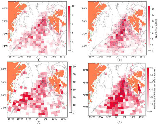
Figure 7.
Number of eddies identified per spatial bin in SST (a) and chl-a (b) data. Probability of eddies identified in SST (c) and chl-a (d) data. Location of each eddy center is shown with blue dot.
However, the most correct way to identify the true eddy generation hot-spots is to look at spatial maps of the probability of eddies obtained by normalization of the total number of eddies per spatial bin (Figure 7a,b) by the corresponding number of data pixels multiplied by 106 per spatial bin. The resulting probability maps are shown in Figure 7c,d and have some pronounced differences compared to Figure 7a,b. The peak eddy activity in SST data has now shifted to the SW part of the region where the EGC passes along the shelf/slope boundary of the Greenland Sea. High eddy probability values in SST data are also detected at 73.5–74°N, 0–5°E, and in the central Fram Strait at 76.5–80°N, 0–7°E, coinciding with the known locations of the AW recirculation branches [26,28].
In chl-a data, the band of the highest eddy probability is observed in the middle between the EGC and the WSC, i.e., in the central Fram Strait. Note also the region of high eddy probability in the western part of Storfjorden (southeast coast of Spitsbergen). Notably, chl-a data also depicts a band of enhanced eddy probability along the trajectory of the WSC south and west of Svalbard.
The difference between spatial distributions of cyclonic and anticyclonic eddies identified in both data sources is visualized by plotting probability of eddies of each type (Figure 8).
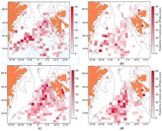
Figure 8.
Probability of cyclonic (a) and anticyclonic (b) eddies identified in SST data. Probability of cyclonic (c) and anticyclonic (d) eddies identified in chl-a data.
Judging from SST data (Figure 8a,b), most of the CEs (264 in total) appear on the line 80°N, 10°E–74°N, 15°W and are rather evenly spread over the other locations (Figure 8a), while ACEs (167 in total) are limited to the western part of the study region and are rare south and south-west of Svalbard (Figure 8b). In some regions, the high probabilities of CEs and ACEs correspond, meaning that many of them formed dipoles. Note also that ACEs are almost absent over the shallow Svalbard shelf, while many CEs populate its western part.
In chl-a data (Figure 8c,d), CEs (365 in total) mostly appear on the line 79°N, 8°E–76°N, 2°E (Figure 8c), i.e., in the northern part of the Fram Strait. In turn, the maximum probability values of ACEs (272 in total) are found to the south of maximum probability of CEs (Figure 8d). The spatial difference in areas where cyclones and anticyclones dominate in chl-a data is an interesting feature deserving further investigation.
3.3. Size and Shape of Eddies
According to Table 1 and Table 2, the mean radii of eddies identified in both data sources are identical, meaning that SST and chl-a fields reveal the same eddy scales. According to Figure 9, radii of cyclones peak at 5–10 km while those of anticyclones are higher, peaking at 10–15 km. Mean radii of cyclones and anticyclones are, respectively, 11.1 km and 14.5 km according to SST data, and 11.8 km and 14.3 km according to chl-a data. So, on the mean, cyclones are typically smaller than anticyclones. In SST data, cyclones strongly prevail over anticyclones within the range of eddy radii of 1–10 km (Figure 9a). Above that, anticyclones start to lead but only a little. In chl-a data, the prevalence of cyclones is within a wider range of 1–15 km, while in the range of 15–30 km the dominance of anticyclones is much more pronounced than in the SST data (Figure 9b).
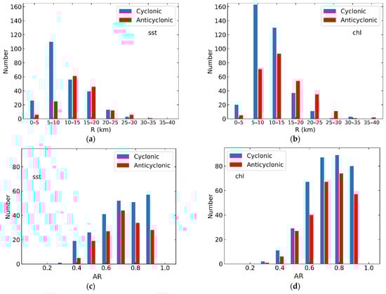
Figure 9.
Histogram distributions of eddy radii R (a,b) and aspect ratio of eddy axes AR (c,d) in SST (a,c) and chl-a (b,d) data for cyclonic (blue bars) and anticyclonic (red bars) eddies identified in 2007 and 2018–2020.
The AR of eddy axes, i.e., the ratio of Amin to Amaj, is different in SST and chl-a datasets (Figure 9c,d). In SST data, the AR histograms for cyclonic and anticyclonic eddies have peaks at different modes, i.e., at 0.9 and 0.7, respectively, meaning that ACEs are more elliptical than CEs in SST data (Figure 9c). In the chl-a data, the difference in the AR between cyclones and anticyclones is less pronounced, with identical modes at 0.8 (Figure 9d). In other words, cyclonic eddies identified in SST data are the most “round”, followed by slightly more elliptical eddies in chl-a data. The most elliptical eddies are anticyclones identified in SST data. In general, the portion of highly elliptical eddies (AR < 0.7) in the SST data is a bit higher (~35%) than that in the chl-a data (~30%).
The spatial distributions of eddy radii and their ARs are shown in Figure 10. In general, both data sources show higher mean eddy radii over deep water compared to shallow coastal regions. This is especially pronounced in chl-a data. The lowest values of mean eddy radii ~5 km in both data sources are found around Svalbard and in the vicinity of Bear Island. However, in SST data, similarly low values are also observed in some locations of the Fram Strait and over the northwestern shelf of the Greenland Sea. In SST data, the maximal mean eddy radii (~20–25 km) are found over the southwestern shelf of the Greenland Sea and around 75°N, 5°W, while in chl-a data higher eddy radii are seen over the deep water in the central Fram Strait.
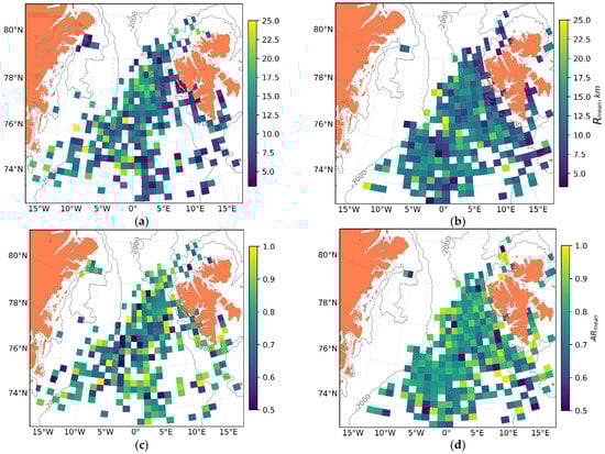
Figure 10.
Spatial distributions of eddy radii R (a,b) and aspect ratio of eddy axes AR (c,d) identified in SST (a,c) and chl-a (b,d) data for eddies identified in 2007 and 2018–2020.
The distributions of ARs of eddies in both data sources seem to be reversed compared to those of R (compare Figure 10a,b with Figure 10c,d). In SST data, highly elliptical (AR < 0.7) and nearly circular (AR > 0.9) eddies could be found almost everywhere. Yet, the most elliptical eddies with AR values of 0.5–0.7 dominate along the trajectory of the EGC south of 79°N. In chl-a data, AR values are more homogeneous in space, yet highly-elliptical eddies are found north of Svalbard, at 73.5°N, 7°W and west of Bear Island. The overall comparison of the results about eddy sizes and shapes suggests that, despite their rather similar ranges of magnitude, the spatial variability of these properties is rather strong and differ quite substantially between SST and chl-a data.
Figure 11 shows a dependence of eddy AR on eddy R separately for cyclones and anticyclones. The most informative part of the plots is for eddy radii bins of 5–20 km because they are mostly populated by observations. From the first glance, there is no obvious dependence of AR on R. Nevertheless, certain tendencies of AR behavior are seen for the particular eddy sign and radius range.
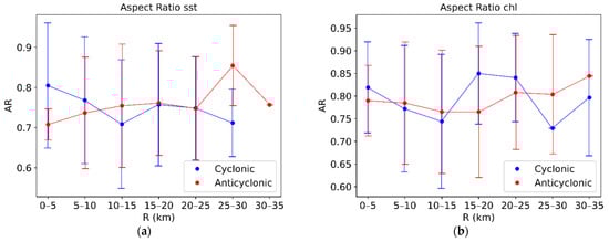
Figure 11.
Variations of eddy AR as a funtion of eddy radius according to SST (a) and chl-a (b) data. Averaged in an eddy-radius bin of 5 km. Vertical lines denote one standard deviation.
First, for the 0–15 km radii range, the AR of cyclones decreases by ~0.1 in both data sources, i.e., CEs become more elliptical with an increase of eddy radii. Then, it slightly (strongly) rises over a 15–25 km radii range in SST (chl-a) data, and falls down again over a 25–30 km radii bin. In chl-a data extending to a 30–35 km bin, the AR of CEs rises again (Figure 11b). So, the overall mean tendency for cyclones, at least in SST data, is to become more elliptical while growing in size.
For anticyclones, the level of AR values is rather stable and only slightly increasing with an increase of eddy radii, i.e., larger ACEs tend to be more circular than smaller ACEs. A single pronounced peak in the AR is seen only in SST data over a 25–30 km bin. The mean level of AR values for anticyclones in the SST and the chl-a data is similar, 0.75 and 0.78, respectively.
Here we may conclude that identification of eddies based on SST and chl-a data produces nearly the same result for cyclones and anticyclones in terms of their size and aspect ratio. While being statistically not significant, the AR of cyclones and anticyclones seem to have a slightly inverse relationship on eddy radii. A rather high number of elliptical eddies suggests that many of them are nonlinear or submesoscale.
3.4. Eddy Dynamics and Trajectories
We have also attempted to track eddies in sequential chl-a data to get their translation speed and direction. Due to frequent cloud cover, it was only possible to track 22 eddies. The period of observations of a particular eddy varied from 1 to 10 days during which from two to four MODIS chl-a maps were available depicting the same eddy. As a result, we have estimated the range of eddy translation velocities of 0.9–9.6 km/day with a mean (median) value of 4.2 (3.3) km/day.
Figure 12a shows a chl-a map of 21 June 2020 where circles of different color mark the locations of six eddies detected on 17–22 June 2020. Figure 12b shows the trajectories of all eddies tracked in 2007 and 2018–2020 with blue and red arrows corresponding to CEs and ACEs, respectively. Note that the arrow length is not proportional to the translation speed, but simply shows the actual trajectory of eddy movement.
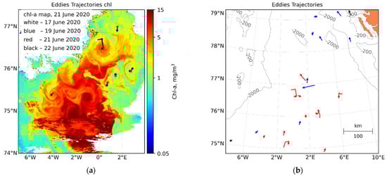
Figure 12.
Analysis of eddy translation velocities from sequential MODIS observations: (a) the chl-a map acquired on 21 June 2020, where dots of different color mark locations of eddies at different dates; (b) the total map with trajectories of all eddies tracked in the analysis with red, blue and black arrows showing trajectories of anticyclones, cyclones and eddies with no recognizable rotation sign.
As seen from Figure 12b, about half of the detected eddies propagate northward, especially those found west of Svalbard. The others travel either westward or southward. The obtained eddy translation speeds and directions seem to be in general agreement with previous findings and the overall scheme of circulation regime in this region (see, e.g., [26,28,34]).
3.5. Eddy-Induced SST and chl-a Anomalies
As described above in Section 2, a qualitative analysis of eddy-induced anomalies in SST/chl-a fields includes three types of eddies with higher, lower and uncertain values of SST/chl-a relative to ambient water. Table 3 summarizes the obtained results for all CEs and ACEs revealed in SST/chl-a data. It is worth mentioning that it was difficult to define the sign of anomalies for about 15% (9.5%) of all eddies detected in SST (chl-a) data, independent of eddy vorticity sign.
Table 3.
Number of eddies in assigned to each type of eddy in terms of eddy core SST and chl-a relationship to surrounding SST and chl-a. Number of eddies is given outside brackets; percentage is given in brackets.
In regard to eddy-induced SST anomalies, no distinct difference is obtained between CEs and ACEs. They all have just a slightly higher percentage of those with a positive SST anomaly compared to those with a negative one. For CEs, the share of eddies with positive SST anomaly is only 4.5% higher than those with a negative anomaly, while for ACEs they are nearly equal.
The differences in eddy-induced chl-a anomalies are more prominent. About 61% of CEs were characterized by a positive chl-a anomaly, while a negative one was found only in 30% of cases. For ACEs, a positive chl-a anomaly was observed in 50% of cases, i.e., 10% more frequently than a negative one.
To sum up, most frequently CEs have positive SST and chl-a anomalies, while negative anomalies are observed only in 40% and 30% of cases, respectively. For ACEs, the probability of encountering positive chl-a anomalies is ~10% higher than a negative one, while positive/negative SST anomalies are detected equally frequently.
4. Discussion
In this work we have attempted to explore the potential of satellite MODIS optical data to gain some knowledge on eddy generation hot-spots and their properties in the key entrance region to the Arctic Ocean—the northern Greenland Sea and the Fram Strait. Our results show that despite frequent cloud and ice cover in the study region, MODIS data enable us to obtain rather rich statistics on eddy generation hot-spots, their spatial properties, dynamics and associated SST and chl-a anomalies.
It is interesting to compare our results in terms of the total number of eddies detected with those based on satellite altimetry and SAR observations and a high-resolution model [34]. In our work, on average 110 (180) eddies were detected per 6 months from April to September in SST (chl-a) data. Analysis of satellite altimetry data for July–September 2007 allowed us to detect 125 mesoscale eddies over the same region [34]. On average, this is about two times more eddies than in SST and chl-a data.
Analysis of SAR data enabled to detect ~2000 eddies from July–September 2007 [34,63], which is about 40 (20) times more than on average registered in the SST (chl-a) data per 4 years. The difference in the number of detected eddies between our results and the high-resolution eddy-resolving Finite-Element Sea Ice–Ocean Model (FESOM) is even more pronounced. The latter has captured more than 2000 eddies per month of 2007 [34], i.e., about two orders of magnitude more than on average in our study. Such big differences are mainly caused by the limiting factors of cloud and ice cover, but some eddies could be also obscured by thermal stratification of the underlying surface layer [20].
The obtained results about the dominance of cyclones versus anticyclones are in line with those obtained earlier from SAR observations [34,36,37,50]. Yet, in our study the ratio of CEs versus ACEs is lower (~60% of CEs vs. ~40% of ACEs) than in SAR data (70–80% vs. 20–30%, respectively). This could be partially explained by the larger size of eddies detected in our study compared to those detected in SAR, i.e., a mean radii of 12 km in MODIS SST/chl-a data versus ~4 km in SAR data. The latter is equal to or smaller than the first Rossby radius of deformation in the Fram Strait in summer, i.e., 4–6 km [3,32], meaning that SAR better captures submesoscale eddies, while MODIS is more effective in observing small mesoscale eddies.
The previous works also show that the larger the eddy radii is relative to the first Rossby radius of deformation, the smaller the difference is in the relative numbers of CEs and ACEs (e.g., [50,64]). That is why altimetry-based statistics for the same region showed approximate parity between CEs and ACEs [7,34]. In turn, the SAR data showed a larger prevalence of CEs because most of the detected eddies were submesoscale. In this respect, the MODIS data with a 1 km spatial resolution captures identical eddy scales as a high-resolution FESOM model. They have similar ranges of eddy radii, 1–30 km, both peaking at 10–15 km, and resolving both submesoscale and mesoscale eddies.
In terms of eddy eccentricity, , the mean eddies’ AR value of 0.77 obtained from MODIS data translates to mean an eccentricity of 0.64. The latter is somewhat smaller than a global average of 0.78 and the range of 0.74–0.79 obtained for our study region from satellite altimetry data [65]. Though Chen et al. [65] show a general poleward decrease of eddy eccentricity for both hemispheres, their estimates are much higher than ours. Most probably, such a discrepancy is again related to different scales of observed eddies, i.e., the altimetry-based large mesoscale eddies with a lifetime of more than one month seem to have a higher eccentricity (are more elliptical) than short-lived small mesoscale and submesoscale eddies observed in MODIS data.
We should also note a high interannual variability in the number of detected eddies, which is different for SST and chl-a data. The latter generally allows us to capture ~1.5 more eddy features than SST data. In both data sources, the total number of eddy detections varies significantly (two to three times) from year to year. The highest number of eddies was registered in 2019 in both data sources, while the lowest one was detected in 2018 in SST data and in 2020 in chl-a data. The interannual variability of eddy observations should be directly related to the background cloud- and ice-cover conditions, which are identical for SST and chl-a data. However, the observed difference in eddy detection results between SST and chl-a data is an interesting fact and deserves further investigation.
Monthly variations in the total number of identified eddies have a maximum in June according to both data sources. After data normalization, the highest portion of eddies identified in SST data were detected from June to August. For chl-a data, most of them were detected in April and June which agrees with the results obtained in [40]. The latter is plausibly linked to the seasonal variations of phytoplankton concentration, i.e., there could be more/less phytoplankton and, hence, more/fewer passive tracers to facilitate eddy identification during particular months in spring and autumn. Moreover, certain effects could be associated with seasonal variations of wind and wave regimes and surface heat fluxes. In particular, they could erase the contrast of surface eddy signatures against the background field due to enhanced mixing or intensified cooling/heating leading to missing some eddies. Though the study region is characterized by the strongest winds and waves across the entire Arctic [66], the latter are less intense during May–August when most of the satellite data used were collected [66,67,68]. The surface heat flux also has a certain monthly variability with a strong warming of the surface layer occurring in June–July and prevailing cooling events in April and September [69].
Locations of eddies have some interesting peculiarities. First, as Figure 1 clearly depicts, SST data shows well-traced surface patterns of two distinct boundary currents, the cold EGC in the west, the warm WSC in the east, and the intermediate “buffer zone” between them where surface waters are actively mixed. In chl-a data, the most pronounced area in terms of chl-a concentration is found exactly over this intermediate “buffer zone” in the central Fram Strait (Figure 1b). As a result, most eddies in chl-a data are detected within this “buffer zone” and its outer boundaries, including the WSC pathway, quite similar to results of recent altimetry observations [7]. In SST, the highest number of eddies is found along the WSC at 78–80°N, i.e., the region characterized by the highest eddy kinetic energy [21] and coinciding with the known locations of the AW recirculation branches [26,28]. However, the highest eddy probability is found along the EGC in the Nordbukta region at 76–78°N, in agreement with Bashmachnikov et al. [34].
Our results show that CEs are more often observed over shallow water, e.g., on the Svalbard shelf, than ACEs. Similar results were obtained in model study by Wekerle et al. [28], showing that CEs tend to stay on the shelf and populate the narrow Svalbard fjords, while anticyclones tend to leave the shallow shelf and travel westward into the deep basin. Following Cushman-Roisin [66], Wekerle et al. [28] suggest that such an asymmetric pathway of eddies generated on the Svalbard shelf and in the WSC region have dynamical causes. In particular, it is explained by an increase/decrease in relative vorticity of eddies and surrounding fluid parcels when they move to deeper/shallower waters. A secondary drift of eddies arising in this case would move cyclones toward shallower water and anticyclones to deeper regions. It is also linked to specific features of the meandering of local water masses when the active generation of cyclones occurs on the shallow eastern side of the shelf along the Svalbard Coastal Current, while the intense generation of anticyclones happens on the deeper western side of the shelf along the warm and salty WSC (see [28] for more details).
In terms of eddy-induced SST and chl-a anomalies, our results show that the overall number of eddies with a positive chl-a anomaly (~62%) is larger than that with a negative one (~38%). For SST, the number of eddies with a positive SST anomaly is only a little higher (~52%) than that with a negative one (~48%). We do not see any large differences between cyclones and anticyclones in terms of their SST anomalies of both signs. However, CEs have a positive chl-a anomaly more often than a negative one, ~61% vs. 30%, compared to anticyclones, ~50% vs. 41%. However, it is unclear whether the elevated chl-a values in eddies is a result of eddy-induced vertical transport or they simply trap chlorophyll-rich water and transport it horizontally.
It is interesting to compare our results with those of Dong et al. [40], who used satellite altimetry, scatterometry and ocean color products to study the chl-a concentration anomalies induced by mesoscale eddies in the northern Norwegian Sea. In particular, they found a dominance of positive chl-a anomalies in ACEs and negative chl-a anomalies within CEs triggered by Ekman pumping due to wind–eddy interactions. In our case, positive chl-a are also frequently found in the ACEs, but they are registered more often within CEs which has some disagreement with Dong et al. [40]. This discrepancy is probably related to the fact that we primarily observe small mesoscale and submesoscale eddies having different properties compared to the large mesoscale eddies considered in [40].
We should also note that the use of standard MODIS chl-a products might be not the best way to assess the eddy-induced surface chl-a variations, and some specific regional in situ-based algorithms should be used instead (like those described in [67,68,69,70]). However, as we use these data to get an overall qualitative understanding of eddy influence on surface chl-a properties, it seems suitable for such a purpose and is often used in other Arctic and subarctic regions [38,40].
An attempt to infer eddy translation properties from sequential MODIS observations has shown that, due to an intensive cloud cover, this is possible only for a very small number of cases. In turn, standardly used satellite altimetry data seem more effective for this purpose [7,34,38]. Nevertheless, the obtained eddy translation directions coincide with the pathway of the topographically trapped WSC (northward traveling eddies) and its recirculation branches (westward and southwestward traveling eddies), in similarity with satellite altimetry and high-resolution FESOM results in this region [34]. Eddy translation speeds (~4 km/day or 4–5 cm/s) also seem to be quite realistic, assuming that some of them might be advected by the mean flows.
5. Conclusions
Here we use two “traditional” satellite remote sensing products—spatial SST and chl-a maps from MODIS Aqua—in attempt to study eddy activity and their properties in the key Arctic region: the northern Greenland Sea and the Fram Strait. Basic statistics derived from SST and chl-a data imply that MODIS Aqua data with a 1 km spatial resolution allow us to study submesoscale and mesoscale eddies within the range of eddy radii of 2–40 km (mean value of 12 km). Most radii of CEs are within 5–10 km, while those of ACEs are higher, in the range of 10–15 km.
According to SST (chl-a) data, the number of cyclones is ~1.6 (~1.3) times greater than that of anticyclones. Most of the eddies are observed in June, and the number of CEs is higher than that of ACEs both during the warm season and interannually. Eddy generation hot-spots are found along and between the main boundary currents of the region—the West Spitsbergen Current and its recirculation branches, the East Greenland Current with the highest eddy probability found in the Nordbukta region and on shelf regions around Svalbard. Notably, the regions where cyclones/anticyclones prevail also differ quite substantially.
The comparison of the results about eddy sizes and shapes suggests that, despite them having rather similar ranges of magnitude, the spatial variability of these properties is rather strong and differ between SST and chl-a data. The mean AR of eddy axes, characterizing their ellipticity, is about 0.77, which means that many of the observed eddies are nonlinear. Though not being statistically significant, the shape of cyclones and anticyclones seem to have an inverse relationship on their radii with CEs (ACEs) becoming more elliptical (circular) while growing.
Mean eddy translation velocities derived from a limited number of sequential observations are about ~4 km/day (4–5 cm/s), which is quite realistic, while their directions correspond to the direction of mean flows.
The number of eddies with a positive SST anomaly is a little higher (~52%) than that with a negative one (~48%). There are no big differences between CEs and ACEs in terms of their SST anomalies of both signs. Yet, the number of eddies with a positive chl-a anomaly (~62%) is larger than that with a negative one (~38%), and CEs more often have a positive chl-a anomaly than ACEs.
Though formally chl-a maps enable us to detect more eddies compared to SST data, they show somewhat different results in terms of eddy generation hot-spots and seasonal variability. Hence, there are no direct winner between them; rather, each data source is suitable for solving a particular task. All in all, we conclude that satellite SST and chl-a data are capable of providing useful information about eddies in the study region on their own, and the statistics obtained from these data are in line and compliment the previous results obtained from SAR, altimetry and high-resolution models.
The main advantage of MODIS data is a capability to directly relate the observed eddy features to actual thermal and/or biological structures of the study region and potentially assess the eddy-induced modulation of these properties. It is also more straightforward and intuitive to use these data for the intercomparison and validation of high-resolution model results compared to gridded satellite altimetry fields of sea surface height anomalies and/or SAR data linked to complex sea surface roughness variations.
The proposed method of MODIS optical data analysis seems to work effectively in other ocean regions as well. Its applicability depends on two main aspects, namely, the data quality/availability and the strength of spatial gradients of chl-a and SST in the data. Obviously, the quality of the data in terms of contamination by clouds/ice would increase toward the equator, which is a primary reason to expect a better performance of the method equatorward. However, the number of intersecting satellite overpasses would decrease toward the equator, which might limit the ability to track individual eddies at short timescales. The method might be also not very efficient in the extreme case of oligotrophic open ocean where the spatial gradients of optical properties are not pronounced. Nevertheless, we believe that the method used here is applicable to practically any ocean region.
Future work should address automation of the eddy identification and processing schemes to reduce possible expert-related biases. Other major goals would also be an extension of the present data set to monitor possible changes and an evolution of the eddy field in the changing Arctic Ocean due to “atlantification” and further reduction of ice cover.
Author Contributions
Conceptualization, I.E.K.; methodology, E.A.M. and I.E.K.; software, E.A.M.; formal analysis, E.A.M. and I.E.K.; investigation, E.A.M. and I.E.K.; resources, E.A.M. and I.E.K.; data curation, E.A.M.; writing—original draft preparation, E.A.M. and I.E.K.; writing—review and editing, E.A.M. and I.E.K.; visualization, E.A.M.; supervision, E.A.M. and I.E.K.; project administration, I.E.K.; funding acquisition, I.E.K. All authors have read and agreed to the published version of the manuscript.
Funding
This research was funded by the Russian Science Foundation, grant number 21-17-00278, https://rscf.ru/project/21-17-00278 (accessed on 13 January 2023).
Data Availability Statement
MODIS Aqua data used in this study are freely available from https://oceancolor.gsfc.nasa.gov (accessed on 15 August 2022).
Conflicts of Interest
The authors declare no conflict of interest.
References
- Mensa, J.A.; Timmermans, M.-L.; Kozlov, I.E.; Williams, W.J.; Özgökmen, T. Surface drifter observations from the Arctic Ocean’s Beaufort Sea: Evidence for submesoscale dynamics. J. Geophys. Res. Oceans 2018, 123, 2635–2645. [Google Scholar] [CrossRef]
- Wang, Q.; Koldunov, N.V.; Danilov, S.; Sidorenko, D.; Wekerle, C.; Scholz, P.; Bashmachnikov, I.L.; Jung, T. Eddy kinetic energy in the Arctic Ocean from a global simulation with a 1-km Arctic. Geophys. Res. Lett. 2020, 47, e2020GL088550. [Google Scholar] [CrossRef]
- von Appen, W.-J.; Wekerle, C.; Hehemann, L.; Schourup-Kristensen, V.; Konrad, C.; Iversen, M.H. Observations of a submesoscale cyclonic filament in the marginal ice zone. Geophys. Res. Lett. 2018, 45, 6141–6149. [Google Scholar] [CrossRef]
- Fine, E.C.; MacKinnon, J.A.; Alford, M.H.; Mickett, J.B. Microstructure observations of turbulent heat fluxes in a warm-core Canada Basin eddy. J. Phys. Oceanogr. 2018, 48, 2397–2418. [Google Scholar] [CrossRef]
- Rippeth, T.P.; Fine, E.C. Turbulent mixing in a changing Arctic Ocean. Oceanography 2022, 35, 66–75. [Google Scholar] [CrossRef]
- Manucharyan, G.E.; Thompson, A.F. Heavy footprints of upper-ocean eddies on weakened Arctic sea ice in marginal ice zones. Nat. Commun. 2022, 13, 2147. [Google Scholar] [CrossRef]
- Bashmachnikov, I.L.; Raj, R.P.; Golubkin, P.; Kozlov, I.E. Heat transport by mesoscale eddies in the Norwegian and Greenland seas. J. Geophys. Res. Oceans 2023, 128, e2022JC018987. [Google Scholar] [CrossRef]
- Watanabe, E.; Onodera, J.; Harada, N.; Honda, M.C.; Kimoto, K.; Kikuchi, T.; Nishino, S.; Matsuno, K.; Yamaguchi, A.; Ishida, A.; et al. Enhanced role of eddies in the Arctic marine biological pump. Nat. Commun. 2014, 5, 3950. [Google Scholar] [CrossRef]
- Kaiser, P.; Hagen, W.; von Appen, W.-J.; Niehoff, B.; Hildebrandt, N.; Auel, H. Effects of a Submesoscale Oceanographic Filament on Zooplankton Dynamics in the Arctic Marginal Ice Zone. Front. Mar. Sci. 2021, 8, 625395. [Google Scholar] [CrossRef]
- Schourup-Kristensen, V.; Wekerle, C.; Danilov, S.; Völker, C. Seasonality of mesoscale phytoplankton control in eastern Fram Strait. J. Geophys. Res. Oceans 2021, 126, e2021JC017279. [Google Scholar] [CrossRef]
- Hunkins, K.L. Subsurface eddies in the Arctic Ocean. Deep Sea Res. Oceanogr. Abstr. 1974, 21, 1017–1033. [Google Scholar] [CrossRef]
- Newton, J.L.; Aagaard, K.; Coachman, L.K. Baroclinic eddies in the Arctic Ocean. Deep Sea Res. Oceanogr. Abstr. 1974, 21, 707–719. [Google Scholar] [CrossRef]
- Manley, T.O.; Hunkins, K. Mesoscale eddies of the Arctic Ocean. J. Geophys. Res. 1985, 90, 4911–4930. [Google Scholar] [CrossRef]
- Johannessen, J.A.; Johannessen, O.M.; Svendsen, E.; Shuchman, R.; Manley, T.; Campbell, W.J.; Josberger, E.G.; Sandven, S.; Gascard, J.C.; Olaussen, T.; et al. Mesoscale eddies in the Fram Strait marginal ice zone during the 1983 and 1984 Marginal IceZone Experiments. J. Geophys. Res. Oceans 1987, 92, 6754–6772. [Google Scholar] [CrossRef]
- Padman, L.; Levine, M.; Dillon, T.; Morison, J.; Pinkel, R. Hydrography and Microstructure of an Arctic Cyclonic Eddy. J. Geophys. Res. 1990, 95, 9411–9420. [Google Scholar] [CrossRef]
- Muench, R.D.; Gunn, J.T.; Whitledge, T.E.; Schlosser, P.; Smethie, W. An Arctic Ocean cold core eddy. J. Geophys. Res. 2000, 105, 23997–24006. [Google Scholar] [CrossRef]
- Timmermans, M.-L.; Toole, J.; Proshutinsky, A.; Krishfield, R.; Plueddemann, A. Eddies in the Canada Basin, Arctic Ocean, observed from ice-tethered profilers. J. Phys. Oceanogr. 2008, 38, 133–145. [Google Scholar] [CrossRef]
- Pnyushkov, A.V.; Polyakov, I.V.; Rember, R.; Ivanov, V.V.; Alkire, M.B.; Ashik, I.M.; Baumann, T.M.; Alekseev, G.V.; Sundfjord, A. Heat, salt, and volume transports in the eastern Eurasian Basin of the Arctic Ocean from 2 years of mooring observations. Ocean Sci. 2018, 14, 1349–1371. [Google Scholar] [CrossRef]
- Brenner, S.; Rainville, L.; Thomson, J.; Lee, C. The evolution of a shallow front in the Arctic marginal ice zone. Elem. Sci. Anthr. 2020, 8, 17. [Google Scholar] [CrossRef]
- Porter, M.; Henley, S.F.; Orkney, A.; Bouman, H.A.; Hwang, B.; Dumont, E.; Venables, E.J.; Cottier, F. A polar surface eddy obscured by thermal stratification. Geophys. Res. Lett. 2020, 47, e2019GL086281. [Google Scholar] [CrossRef]
- von Appen, W.-J.; Alfred Wegener Institute; Baumann, T.; Janout, M.; Koldunov, N.; Lenn, Y.-D.; Pickart, R.; Scott, R.; Wang, Q. Eddies and the distribution of eddy kinetic energy in the Arctic Ocean. Oceanography 2022, 35, 42–51. [Google Scholar] [CrossRef]
- Rabe, B.; Heuzé, C.; Regnery, J.; Aksenov, Y.; Allerholt, J.; Athanase, M.; Bai, Y.; Basque, C.; Bauch, D.; Baumann, T.M.; et al. Overview of the MOSAiC expedition: Physical oceanography. Elem. Sci. Anthr. 2022, 10, 00062. [Google Scholar] [CrossRef]
- Zhao, M.; Timmermans, M.L.; Cole, S.; Krishfield, R.; Proshutinsky, A.; Toole, J. Characterizing the eddy field in the Arctic Ocean halocline. J. Geophys. Res. Oceans 2014, 119, 8800–8817. [Google Scholar] [CrossRef]
- Zhang, K.; Song, H.; Coakley, B.; Yang, S.; Fan, W. Investigating Eddies From Coincident Seismic and Hydrographic Measurements in the Chukchi Borderlands, the Western Arctic Ocean. J. Geophys. Res. Oceans 2022, 127, 10. [Google Scholar] [CrossRef]
- Spall, M.A.; Pickart, R.S.; Fratantoni, P.S.; Plueddemann, A.J. Western Arctic shelf break eddies: Formation and transport. J. Phys. Oceanogr. 2008, 38, 1644–1668. [Google Scholar] [CrossRef]
- Hattermann, T.; Isachsen, P.E.; Isachsen, P.E.; von Appen, W.-J.; Albretsen, J.; Sundfjord, A. Eddy-driven recirculation of Atlantic Water in Fram Strait. Geophys. Res. Lett. 2016, 43, 3406–3414. [Google Scholar] [CrossRef]
- Crews, L.; Sundfjord, A.; Albretsen, J.; Hattermann, T. Mesoscale eddy activity and transport in the Atlantic Water inflow region north of Svalbard. J. Geophys. Res. Oceans 2018, 123, 201–215. [Google Scholar] [CrossRef]
- Wekerle, C.; Hattermann, T.; Wang, Q.; Crews, L.; von Appen, W.-J.; Danilov, S. Properties and dynamics of mesoscale eddies in Fram Strait from a comparison between two high-resolution ocean–sea ice models. Ocean Sci. 2020, 16, 1225–1246. [Google Scholar] [CrossRef]
- Platov, G.; Golubeva, E. Characteristics of mesoscale eddies of Arctic marginal seas: Results of numerical modeling. IOP Conf. Ser. Earth Environ. Sci. 2020, 611, 012009. [Google Scholar] [CrossRef]
- Meneghello, G.; Marshall, J.; Lique, C.; Isachsen, P.E.; Doddridge, E.; Campin, J.-M.; Regan, H.; Talandier, C. Genesis and Decay of Mesoscale Baroclinic eddies in the seasonally ice-covered interior Arctic Ocean. J. Phys. Oceanogr. 2021, 51, 115–129. [Google Scholar] [CrossRef]
- MacKinnon, J.A.; Simmons, H.L.; Hargrove, J.; Thomson, J.; Peacock, T.; Alford, M.H.; Barton, B.I.; Boury, S.; Brenner, S.D.; Couto, N.; et al. A warm jet in a cold ocean. Nat. Commun. 2021, 12, 2418. [Google Scholar] [CrossRef] [PubMed]
- Nurser, A.J.G.; Bacon, S. The Rossby radius in the Arctic Ocean. Ocean Sci. 2014, 10, 967–975. [Google Scholar] [CrossRef]
- Timmermans, M.-L.; Marshall, J. Understanding Arctic Oceancirculation: A review of ocean dynamics in a changing climate. J. Geophys. Res. Oceans 2020, 125, e2018JC014378. [Google Scholar] [CrossRef]
- Bashmachnikov, I.L.; Kozlov, I.E.; Petrenko, L.A.; Glock, N.I.; Wekerle, C. Eddies in the North Greenland Sea and Fram Strait from satellite altimetry, SAR and high-resolution model data. J. Geophys. Res. Oceans 2020, 125, e2019JC015832. [Google Scholar] [CrossRef]
- Manucharyan, G.E.; Thompson, A.F. Submesoscale sea ice–ocean interactions in marginal ice zones. J. Geophys. Res. Oceans 2017, 122, 9455–9475. [Google Scholar] [CrossRef]
- Atadzhanova, O.A.; Zimin, A.V.; Romanenkov, D.A.; Kozlov, I.E. Satellite radar observations of small eddies in the White, Barents and Kara Seas. Phys. Oceanogr. 2017, 2, 75–83. [Google Scholar] [CrossRef]
- Kozlov, I.E.; Artamonova, A.V.; Manucharyan, G.E.; Kubryakov, A.A. Eddies in the Western Arctic Ocean from spaceborne SAR observations over open ocean and marginal ice zones. J. Geophys. Res. Oceans 2019, 124, 6601–6616. [Google Scholar] [CrossRef]
- Kubryakov, A.A.; Kozlov, I.E.; Manucharyan, G.E. Large mesoscale eddies in the Western Arctic Ocean from satellite altimetry measurements. J. Geophys. Res. Oceans 2021, 126, e2020JC016670. [Google Scholar] [CrossRef]
- Cassianides, A.; Lique, C.; Korosov, A. Ocean Eddy Signature on SAR-Derived Sea Ice Drift and Vorticity. Geophys. Res. Lett. 2021, 48, 6. [Google Scholar] [CrossRef]
- Dong, H.; Zhou, M.; Raj, R.P.; Smith, W.O.; Basedow, S.L.; Ji, R.; Ashjian, C.; Zhang, Z.; Hu, Z. Surface chlorophyll anomalies induced by mesoscale eddy-wind interactions in the northern Norwegian Sea. Front. Mar. Sci. 2022, 9, 1002632. [Google Scholar] [CrossRef]
- Manucharyan, G.E.; Lopez-Acosta, R.; Wilhelmus, M.M. Spinning ice floes reveal intensification of mesoscale eddies in the western Arctic Ocean. Sci. Rep. 2022, 12, 7070. [Google Scholar] [CrossRef] [PubMed]
- Zimin, A.V.; Atazhanova, O.A.; Romanenkov, D.A.; Kozlov, I.E.; Chapron, B. Submesoscale eddies in the White Sea based on satellite radar measurements. Izv. Atmos. Ocean. Phys. 2021, 57, 1705–1711. [Google Scholar] [CrossRef]
- Zhuk, V.; Kozlov, I.; Kubryakov, A.; Solovyov, D.; Osadchiev, A.; Stepanova, N.; Shirshov Institute of Oceanology RAS. Moscow Institute of Physics and Technology Application of UAV measurements to assess the dynamics of the marginal ice zone in the Kara Sea. Curr. Probl. Remote Sens. Earth Space 2022, 19, 235–245. [Google Scholar] [CrossRef]
- Klenke, M.; Schenke, H.W. A new bathymetric model for the central Fram Strait. Mar. Geophys. Res. 2002, 23, 367–378. [Google Scholar] [CrossRef]
- von Appen, W.-J.; Schauer, U.; Hattermann, T.; Beszczynska-Möller, A. Seasonal Cycle of Mesoscale Instability of the West Spitsbergen Current. J. Phys. Oceanogr. 2016, 46, 1231–1254. [Google Scholar] [CrossRef]
- Cokelet, E.D.; Tervalon, N.; Bellingham, J.G. Hydrography of the West Spitsbergen Current, Svalbard Branch: Autumn 2011. J. Geophys. Res. 2008, 113, C01006. [Google Scholar] [CrossRef]
- Våge, K.; Pickart, R.S.; Pavlov, V.; Lin, P.; Torres, D.J.; Ingvaldsen, R.; Sundfjord, A.; Proshutinsky, A. The Atlantic Water boundary current in the Nansen Basin: Transport and mechanisms of lateral exchange. J. Geophys. Res. Oceans 2016, 121, 6946–6960. [Google Scholar] [CrossRef]
- Pérez-Hernández, M.D.; Pickart, R.S.; Pavlov, V.; Våge, K.; Ingvaldsen, R.; Sundfjord, A.; Renner, A.H.H.; Torres, D.J.; Erofeeva, S.Y. The Atlantic Water boundary current north of Svalbard in late summer. J. Geophys. Res. Oceans 2017, 122, 2269–2290. [Google Scholar] [CrossRef]
- Kozlov, I.E.; Plotnikov, E.V.; Manucharyan, G.E. Brief Communication: Mesoscale and submesoscale dynamics in the marginal ice zone from sequential synthetic aperture radar observations. Cryosphere 2020, 14, 2941–2947. [Google Scholar] [CrossRef]
- Kozlov, I.E.; Atadzhanova, O.A. Eddies in the marginal ice zone of Fram Strait and Svalbard from spaceborne SAR observations in winter. Remote Sens. 2022, 14, 134. [Google Scholar] [CrossRef]
- Watanabe, E. Beaufort shelf break eddies and shelf-basin exchange of Pacific summer water in the western Arctic Ocean detected by satellite and modeling analyses. J. Geophys. Res. 2011, 116, C08034. [Google Scholar] [CrossRef]
- Brown, O.B.; Minnett, P.J.; Evans, R.; Kearns, E.; Kilpatrick, K.; Kumar, A.; Sikorski, R.; Závody, A. MODIS Infrared Sea Surface Temperature Algorithm Algorithm Theoretical Basis Document Version 2.0; University of Miami: Miami, FL, USA, 1999. [Google Scholar]
- Clark, D.K. MODIS Algorithm Theoretical Basis Document Bio-Optical Algorithms—Case 1 Water, Version 1.2; National Oceanic and Atmospheric Administration National Environmental Satellite Service: Washington, DC, USA, 1997.
- Hu, C.; Lee, Z.; Franz, B. Chlorophyll a algorithms for oligotrophic oceans: A novel approach based on three-band reflectance difference. J. Geophys. Res. 2012, 117, C01011. [Google Scholar] [CrossRef]
- SST Reprocessing. 2019. Available online: https://oceancolor.gsfc.nasa.gov/reprocessing/r2019/sst/ (accessed on 10 January 2023).
- NASA Goddard Space Flight Center; Ocean Ecology Laboratory; Ocean Biology Processing Group. Moderate-Resolution Imaging Spectroradiometer (MODIS) Aqua Ocean Color Data; 2018 Reprocessing; NASA OB.DAAC: Greenbelt, MD, USA, 2018. [CrossRef]
- Duda, R.O.; Hart, P.E. Pattern Classification and Scene Analysis; John Wiley & Sons: New York, NY, USA, 1973. [Google Scholar]
- Fernandes, A.M. Study on the Automatic Recognition of Oceanic Eddies in Satellite Images by Ellipse Center Detection—The Iberian Coast Case. IEEE Trans. Geosci. Remote Sens. 2009, 47, 2478–2491. [Google Scholar] [CrossRef]
- Miltiadou, M.; Papoutsa, C.; Karathanassi, V.; Kolokousis, P.; Lafon, V.; Sykas, D.; Sarelli, A.; Prodromou, M.; Hajimitsis, D. Detection of marine fronts: A comparison between different approaches applied on the SST product derived from Sentinel-3 data. In Proceedings of the Sixth International Conference on Remote Sensing and Geoinformation of the Environment (RSCy2018), Paphos, Cyprus, 26–29 March 2018. [Google Scholar] [CrossRef]
- Arrigo, K.R.; van Dijken, G.L. Secular trends in Arctic Ocean net primary production. J. Geophys. Res. 2011, 116, C09011. [Google Scholar] [CrossRef]
- Munk, W.; Armi, L.; Fischer, K.; Zachariasen, F. Spirals on the sea. Proc. R. Soc. Lond. Ser. A Math. Phys. Eng. Sci. 2000, 456, 1217–1280. [Google Scholar] [CrossRef]
- Ni, Q.; Zhai, X.; Wilson, C.; Chen, C.; Chen, D. Submesoscale eddies in the South China Sea. Geophys. Res. Lett. 2021, 48, e2020GL091555. [Google Scholar] [CrossRef]
- Petrenko, L.A.; Kozlov, I.E. Properties of eddies near Svalbard and in Fram Strait from spaceborne SAR observations in summer. Sovr. Probl. DZZ Kosm. 2020, 17, 167–177. [Google Scholar] [CrossRef]
- Chen, G.; Han, G.; Yang, X. On the intrinsic shape of oceanic eddies derived from satellite altimetry. Remote Sens. Environ. 2019, 228, 75–89. [Google Scholar] [CrossRef]
- Stuhlmacher, A.; Gade, M. Statistical analyses of eddies in the Western Mediterranean Sea based on Synthetic Aperture Radar imagery. Remote Sens. Environ. 2020, 250, 112023. [Google Scholar] [CrossRef]
- Cushman-Roisin, B. Introduction to Geophysical Fluid Dynamics; Prentice Hall: Englewood Cliffs, NJ, USA, 1994. [Google Scholar]
- Pavlov, A.K.; Granskog, M.A.; Stedmon, C.A.; Ivanov, B.V.; Hudson, S.R.; Falk-Petersen, S. Contrasting optical properties of surface waters across the Fram Strait and its potential biological implications. J. Mar. Syst. 2015, 143, 62–72. [Google Scholar] [CrossRef]
- Lewis, K.M.; Mitchell, B.G.; Van Dijken, G.L.; Arrigo, K.R. Regional chlorophyll a algorithms in the Arctic Ocean and their effect on satellite-derived primary production estimates. Deep. Sea Res. Part II Top. Stud. Oceanogr. 2016, 130, 14–27. [Google Scholar] [CrossRef]
- Lewis, K.M.; Arrigo, K.R. Ocean color algorithms for estimating chlorophyll a, CDOM absorption, and particle backscattering in the Arctic Ocean. J. Geophys. Res. Oceans 2020, 125, e2019JC015706. [Google Scholar] [CrossRef]
- Korchemkina, E.; Deryagin, D.; Pavlova, M.; Kostyleva, A.; Kozlov, I.E.; Vazyulya, S. Advantage of Regional Algorithms for the Chlorophyll-a Concentration Retrieval from In Situ Optical Measurements in the Kara Sea. J. Mar. Sci. Eng. 2022, 10, 1587. [Google Scholar] [CrossRef]
Disclaimer/Publisher’s Note: The statements, opinions and data contained in all publications are solely those of the individual author(s) and contributor(s) and not of MDPI and/or the editor(s). MDPI and/or the editor(s) disclaim responsibility for any injury to people or property resulting from any ideas, methods, instructions or products referred to in the content. |
© 2023 by the authors. Licensee MDPI, Basel, Switzerland. This article is an open access article distributed under the terms and conditions of the Creative Commons Attribution (CC BY) license (https://creativecommons.org/licenses/by/4.0/).