Abstract
Due to the limitations of current technology and budget, as well as the influence of various factors, obtaining remote sensing images with high-temporal and high-spatial (HTHS) resolution simultaneously is a major challenge. In this paper, we propose the GAN spatiotemporal fusion model Based on multiscale and convolutional block attention module (CBAM) for remote sensing images (MCBAM-GAN) to produce high-quality HTHS fusion images. The model is divided into three stages: multi-level feature extraction, multi-feature fusion, and multi-scale reconstruction. First of all, we use the U-NET structure in the generator to deal with the significant differences in image resolution while avoiding the reduction in resolution due to the limitation of GPU memory. Second, a flexible CBAM module is added to adaptively re-scale the spatial and channel features without increasing the computational cost, to enhance the salient areas and extract more detailed features. Considering that features of different scales play an essential role in the fusion, the idea of multiscale is added to extract features of different scales in different scenes and finally use them in the multi loss reconstruction stage. Finally, to check the validity of MCBAM-GAN model, we test it on LGC and CIA datasets and compare it with the classical algorithm for spatiotemporal fusion. The results show that the model performs well in this paper.
1. Introduction
The continuous development of Earth observation technology promotes the increasing demand for high-temporal and high-spatial (HTHS) remote sensing images [1], which are mainly used in urban resource monitoring [2], crop and forest monitoring [3], scene classification [4], surface object detection and segmentation [5,6], carbon sequestration modeling [7], crop yield prediction [8], and disaster monitoring [9]. However, due to the limitations of current technology and financial budget, it is difficult to obtain simultaneous remote sensing images with HTHS requirements using a single satellite product. To solve this problem, we now combine satellite data from multiple platforms to obtain HTHS images [10]. For example, combining remote sensing images from the high-resolution Landsat and moderate-resolution imaging spectroradiometer (MODIS), the access time of the Landsat series satellites [11] is typically 16 days, and the spatial resolution is 30 m. Such remote sensing images can be used mainly in precision agriculture, land cover classification, and other research areas. The period during which MODIS acquires remote sensing images with low spatial resolution sensors is only one day, and the spatial resolution ranges from 250 to 1000 m [12]. Such images can provide daily remote sensing observations, but it is difficult to observe the very heterogeneous surface changes.
The development of deep learning in the field of computer vision has provided a solid foundation for research in spatiotemporal fusion, so a large number of fusion algorithms based on deep learning have been proposed by researchers. Most of the proposed fusion algorithms are based on the deep convolutional neural network (CNN) model. However, due to the experiential nature of the convolutional kernel, contextual information can only be partially obtained during the reconstruction process. Subsequently, the generative adversarial network (GAN) [13] achieved remarkable results in image enhancement [14], image inpainting [15], and super-resolution reconstruction [16], and gradually applied them to the field of remote sensing images. For example, many spatiotemporal fusion models have been proposed: SRGAN [16], STFGAN [17], GANSTFM [18], CycleGANSTF [19], etc. Although GAN-based spatiotemporal fusion has improved the quality of fusion images, there are still the following problems: (1) The dependence of input image data on time sequence. (2) The characteristics of time and space dimensions are vastly different. Features are complicated. (3) The previous model increases the computation amount of the model when an attention module is added, which increases the running time of the model. (4) Most loss functions ignore image features and visual losses, so the final reconstruction effect does not reach the expected value. This article is committed to solving these existing problems.
In this paper, we design a novel MCBAM-GAN model for spatiotemporal fusion and fully consider the above problems. This model is divided into three stages: multi-level feature extraction, multi-feature fusion, and multi-scale reconstruction. In the generator, we use the U-NET network model and add a convolutional block attention module (CBAM) [20], which can extract the texture features of the image multi-dimensionally and avoid the problem of gradient disappearance and considerable computation to ensure the robustness of the model. Our main contributions are as follows:
- MCBAM-GAN the model of spatiotemporal fusion consists essentially of an encoding-decoding structure. Firstly, the generator part uses the U-NET to deal with the vast resolution difference. The input image is a pair of coarse and fine images. Three encoders are used to completely extract the multi-level features of coarse and fine images. Secondly, the CBAM module and the multi-scale idea are added to the encoder to completely extract detailed features to provide a good foundation for the fusion and reconstruction phase, and the model feature representation is further improved through multi-level feature information. Finally, the multi loss function is used to calculate the accuracy of the image so that a high-quality HTHS remote sensing image can be reconstructed. This structure improves the feature learning ability and has strong generalization.
- The CBAM module is added to the generator. The core idea of this module is to focus on the characteristics of the channel and spatial axis, respectively, and to improve the meaningful characteristics of the channel and spatial axis dimensions by sequentially applying the channel and spatial attention modules. The computational cost is almost negligible. The whole model reduces the number of parameters and saves computation time.
- The model proposed in this paper MCBAM-GAN is compared with the classical spatiotemporal fusion model on the Coleambally Irrigation Area (CIA) dataset and the lower Gwydir catchments (LGC) dataset, and our model achieves good results.
The rest of the papers are arranged as follows. In Section 2 related works on spatiotemporal fusion of remote sensing images are summarized and discussed. In Section 3, we detail an overview of the MCBAM-GAN model framework, generator, discriminator, CBAM module, etc. In Section 4, we perform ablation experiments and experimental analysis to verify the effectiveness of the MCBAM-GAN model. In Section 5, we summarize this paper.
2. Related Works
In recent years, researchers in the field of remote sensing have proposed many fusion algorithms, which can be divided into five categories: decomposition-based methods, weight function-based methods, Bayesian-based methods, hybrid methods, and learning-based methods.
2.1. Decomposition-Based Methods
The decomposition-based methods [21,22,23,24] assume that the land cover does not change between the input and predicted images. Such models based on line-based decomposition are the first to perform spatiotemporal fusion.The principle of the algorithm is simple and easy to use. However, due to the low resolution of the coarse image, it is impossible to accurately decompose each type of surface feature, and it is impossible to obtain good results in different areas with many land cover types. This method is suitable for scenes with fewer land cover types. This method mainly uses linear spectral mixing theory to determine the value of fine pixels by analyzing the composition of coarse pixels and decomposing these coarse pixels.
2.2. Weight Function-Based Methods
The weight-based method is a simple model theory that does not need to learn many parameters from a lot of external data and is therefore fast and stable in most cases. Gao et al. [25] first proposed a Spatio-temporal adaptive reflection fusion model (STARFM) based on a weighting function. STARFM uses a weighting function to predict pixels. The weighting function is calculated from the spectral differences between the data and the information of the neighbouring pixels. The enhanced STARFM (ESTARFM) [26] considers the difference between mixed pixels and pure pixels to modify the weight of STARFM, solve the problem of heterogeneous landscapes, and enhance the ability to monitor seasonal landscape changes. However, it cannot accurately predict the objects whose shape changes with time and the boundaries of fuzzy changes. STAARCH [27] monitors change points from dense time series of coarse images to identify spatial and temporal changes in landscape at a better level of detail. The algorithm SADFAT [28] modifies STARFM and improves the accuracy of heterogeneous landscape prediction by reducing the changes in thermal radiation on fine- and coarse-resolution images through conversion coefficients. However, the algorithm must specify the window size and number of land cover categories and ignores mismatches between Landsat and MODIS pixels. Most weight-based methods are empirical functions that rely on the pixel information of other input images, so it is difficult to extract accurate information from adjacent images when there are too many land cover types or abnormal changes, such as sudden changes in land cover, and the fusion accuracy is low. Moreover, this kind of algorithm cannot reconstruct details because its weighting model is similar to a low-pass filter, which tends to smooth some details.
2.3. Bayesian-Based Methods
The focus of the Bayesian-based fusion method is on modelling the relationship between the observed image and the image to be predicted, taking full advantage of the temporal and spatial relationship, which reduces the prediction accuracy when the type of land cover changes. This method is suitable for scenarios that require high model flexibility. In 2013, the BME algorithm [29] was proposed, which mainly uses the Bayesian maximum entropy mechanism to avoid the complexity and uncertainty caused by image scaling, solve multi-scale problems, and capture fine spatial structure, but it can generate noise during splicing. The NDVI-BSFM algorithm [30] uses constrained decomposition of observation data to obtain more spatial detail and is less dependent on pending prediction data. STS [31] can perform different types of fusion tasks by creating relational models and inverse fusion that is not limited by the number of remote sensing sensors. Bayesian fusion [32] is based on an observational model and a Gaussian distribution. The model framework is flexible, and there is no limit on the number of high-resolution input images. It must effectively extract mixed spectra and limit the potential of retrieval spectra.
2.4. Learning-Based Methods
The learning-based algorithm establishes the appropriate relationship based on the structural similarity of fine and coarse-resolution images, and trains the model using existing datasets to find the relationship between spatiotemporal images. This kind of algorithm can capture the most important features in prediction, including the change of land cover type. However, due to the large scale difference between the coarse and fine images, it cannot accurately maintain the shape of the prediction object, especially that of the object with irregular surface, which is suitable for scenes with large data samples and a long time period. We divide learning-based algorithms into two categories: shallow learning and deep learning. The typical representation for shallow learning method is sparse representation or dictionary learning. For example, the spatiotemporal reflectance fusion model (SPSTFM) [33], one-pair learning [34], EBSPTM [35], and other algorithms have the advantage that they can effectively handle phenological changes and land cover changes, but the calculational cost is large.
2.5. Hybrid Methods
The hybrid spatio-temporal fusion method combines the advantages of the decomposition method, Bayesian theory, weight function, and learning method to achieve a better fusion effect. This method mainly deals with the change of different land cover types, which improves the generalization ability of the model. However, at the same time, it also increases the complexity of the algorithm, which limits its large-scale application. This method is suitable for scenarios with high prediction accuracy and unlimited model complexity. For example, the Spatio-temporal reflection model STRUM [36] proposed in 2015 fuses the changing pixels in the coarse image by using reflectance separation, Bayesian framework, and other methods. In order to obtain the reflectance changes of each type of surface feature information, the model has the advantage of being sensitive to time changes and has good performance in limited high-resolution image data, while the disadvantage is that it cannot extract detailed features very well. STIMFM [37] fusion algorithm adopts spectral decomposition and Bayesian framework, which can achieve high calculation efficiency and image generation accuracy but needs to solve the land cover prediction problem over a long period. flexible spatio-temporal data fusion (FSDAF) [38] combines the two methods of hybrid weighting. The algorithm computes the spectral change of the uniform region, predicts the spatial change by the interpolation algorithm, and finally obtains the high-resolution image using the weighted sum of the spectral and spatial features. The improved FSDAF (SFSDAF) [39] combines sub-pixel fractional change information to more accurately grasp spectral information changes. In FSDAF 2.0 [40], more pure pixels are obtained by edge and change detection, which makes the unmixing process more accurate. At the same time, change detection is also used to generate weights to obtain a more accurate prediction. This method can effectively balance spatial detail preservation and spectral change of reconstruction, but the high complexity of the algorithm limits its wider application.
Deep learning based methods usually use CNN and GAN models, and CNN has robust feature extraction capability under the supervised learning mechanism [41]. In the super-resolution reconstruction of remote sensing images at multiple levels, fusion based on temporal and spatial features has made a breakthrough in recent years, especially in spatiotemporal fusion based on deep learning. The CNN and GAN models are described below. The spatiotemporal fusion algorithm based on CNN (STFDCNN) [42] divides the training phase of this method into two parts. These two parts use the idea of residual network to focus the network on learning high-frequency details. The depth convolution spatiotemporal fusion network (DCSTFN) [43] is a doubly branched convolutional network that effectively fuses spatiotemporal information. It gets by with few reference images and model parameters and is very efficient, but must fully extract fine image features. The extended EDCSTFN [44] added a weight fusion based on double-branch folding. This model mitigates the land cover change problem and can retain high-frequency information, but the number of parameters has increased. StfNet [45] mitigates the problem of spatial information loss in the feature extraction. This method introduces the principles of time dependence and time consistency, so that the image of the predicted date can be combined with the image of the previous date and the image of the following date to obtain the final prediction results. However, some details are lost in the fusion process. There are also bias-driven spatio-temporal fusion models (BiaSTF) [46], spatial, sensor, and temporal spatio-temporal fusion (SSTSTF) [47], residual network ResStf [48], multi-scale, extended convolution DMNet [49], 3D convolution STF3DCNN [50], etc.
Based on the GAN model, it also has many advantages in terms of temporal-spatial fusion. Zhang et al. [17] proposed a spatiotemporal fusion method STFGAN based on the generated countermeasure network. Based on SRGAN [16], more detailed features are extracted, and the prediction results of the generated countermeasure network are more realistic. CycleGANSTF [19] considers image fusion as a data-enhancement problem and selects the image with the most information richness as the fusion result. Tan et al. proposed GANSTFM [18] to alleviate the problem that the model relies too much on the reference image. Song et al. proposed MLFF-GAN [51] to solve the huge difference between high resolution and low resolution. In previous models, one or two groups of reference images are often required, and strict constraints must be applied to the reference images. In order to deal with this problem and improve the prediction accuracy of the model under poor conditions, the conditional production countermeasure network and the switchable normalization module are used to relax the strict constraints on the input image. However, the model parameters are large and difficult to train. To solve these problems, spatio-temporal fusion of remote sensing images based on deep learning is currently crucial for research. For the methods of relevant work parts, we summarized and analyzed according to the classification, and the details are shown in Table 1. Table 1 mainly introduces some models of the five categories of methods, but not all of them. In addition, the latest method based on deep learning is introduced in detail in the article, so it is not added to the table.

Table 1.
Classification Comparison of Spatiotemporal Fusion Algorithms for Remote Sensing Images.
3. Proposed Methods
3.1. Overview
In this paper, a new spatio-temporal fusion method, the MCBAM-GAN model, consisting of a generator and a discriminator is proposed. The generator is designed as a U-NET network structure, which is mainly responsible for transferring the context information to a higher resolution layer, and provides high-quality HTHS images through repeated training, prediction, and fusion of images (see Section 3.3 and Section 3.4 below for a detailed introduction to the model). First, adding multi-scale and convolutional attention modules in the generator to fully extract image features from multiple dimensions while improving the feature learning and generalization ability of the whole model. Second, the image input only needs to predict the time , a pair of coarse and fine images to participate in the spatio-temporal fusion of the whole model, eliminating the restriction on the collection time of reference images and making the time period of and as small as possible. The discriminator is constructed by a residual block based on the ResNet [52] network, which is mainly used to evaluate the generated and actual images. Figure 1 shows the model diagram of the objective problem to be solved.
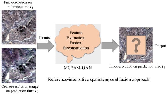
Figure 1.
Objective Problems to be solved in the spatio-temporal fusion model based on deep learning (the model input uses only one coarse resolution image and another arbitrary fine resolution image at the prediction date as reference).
3.2. Overall Framework of MCBAM-GAN Model
The spatiotemporal fusion algorithm based on the deep learning model effectively improves the accuracy of spatiotemporal fusion and provides a better HTHS remote sensing image. Since the spatiotemporal fusion algorithm based on the CNN model is limited by the size of the convolution kernel and cannot extract global image features, this model must solve the following problems: How to extract spatiotemporal difference features at a deeper level; How to extract the global information of two images in the process of time change and reduce the dependence on time series; How to reduce the computation of the fusion model and improve the time efficiency. As shown in Figure 2, that is the overall framework of MCBAM-GAN. The overall network structure is an end-to-end structure. Based on the ideas of GAN model, it is mainly divided into two parts: generator and discriminator [13]. The generator is divided into three stages: multi-feature extraction, multi-feature fusion, and multi-scale reconstruction. In order to reduce the number of input images and the dependence on time series, the input image of the generator consists of a coarse image at time and a fine image at time . Then, the generator has three encoders to precisely merge the input thick and thin image pairs. Finally, the coding is complemented by the CBAM convolutional attention module, which provides adaptive rescling of the spatial and channel features to enhance the salient regions and extract more detailed features. The discriminator based on the resnet structure is mainly used to detect whether the input image is correct or incorrect.
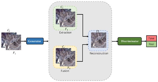
Figure 2.
MCBAM-GAN overall architecture diagram in which the generator phase consists of feature extraction, feature fusion and multi-scale reconstruction (see the insensitive model [18] in the generator phase, where and represent the synthetic fine resolution image and the observed coarse resolution image at the prediction date and time and , respectively). On the input and The features are extracted and fused respectively, and finally the high-quality fine image of the predicted time is reconstructed.
3.3. Generator
Since the GAN was proposed, many image-processing models based on GAN have emerged, and each model has played an influential role in modeling and image processing. GAN consists mainly of a generator-discriminator. Any design based on the GAN model requires a lot of data support. We achieve the balance between the generator and discriminator through multiple iterations of training to improve the model performance of the whole system. Essentially, we can see that the generator and discriminator compete with each other, and the generator has the same incorrect output as the actual data through multiple iterations of training. The discriminator distinguishes whether the output data are actual or false data. Normally, when training the GAN model, we need to make a complex mapping between the noise data of the generator input samples and the actual data. The discriminator uses a binary classifier to distinguish between real and fake data. However, due to many additional constraints on our data during the process of accurate mapping and classification, the stability of the training model could be better. Therefore, many researchers are devoted to improving the stability of the model while reducing the number of parameters. In this model, due to the specificity of the spatiotemporal fusion input data, we choose the least squares GAN (LSGAN) as the generated confrontation loss function [53] expressed as Formulas (2) and (3), and the generated confrontation loss function in this paper is expressed as Formula (1), where:
From a mathematical point of view, generator G uses some noise data z as input to learn the complex mapping function on the real training sample x, and attempts to map the distribution of noise data to the distribution of real data . At the same time, discriminator D is used as a binary classifier to distinguish the generated pseudo data from the real sample x. In other words, the goal of the generator is to minimize the distribution distance between and x, while the goal of the discriminator is to maximize the distribution between them.
In the above discussion, we mentioned that the generator of the model in this paper adopts the U-NET structure. The U-NET is a symmetric network structure that mainly uses the residual block of the residual network (ResNet) as the basic block. The residual block can effectively prevent the gradient explosion and gradient loss [54] of the model. As shown in the overall structure of the generator in Figure 3, in the left structure of the U-NET network, we mainly perform multiple feature extraction. In the right structure, we perform multi-feature fusion and multi-scale reconstruction. In the whole network structure, the size of our convolutional kernel is 3 × 3, and the main task of gencoder is to completely extract global and local coarse and sparse image features. In the first phase, gencoder does not perform downsampling to ensure accuracy. With downsampling, the receptive field increases, the perceptual area per unit area becomes more significant, and the low-frequency information of the image is better perceived. In the second and third stages, gencoder then downsampling the image to obtain more low-frequency information. The main function of the concatenated module is to use different convolution kernels to extract features at different levels. On the right side of Figure 3, the upsampling operation is performed, which helps to integrate the information of each phase of downsampling into the upsampling process and combine the structural information of each level. After the multidimensional feature extraction, we need to complete the multiple feature fusion phase. After the feature extraction module, the algorithm obtains two feature maps that explicitly extract the complementary information of high spatial-low temporal and high temporal-low spatial. Considering that the purpose of spatiotemporal fusion is to obtain remote sensing images with high spatial-temporal resolution at the same time. Therefore, this paper calls the optimized feature fusion module to fuse the extracted feature images. Considering that different feature maps have different contributions to the final result, we use attention feature fusion. To fully fuse the extracted multidimensional features, we use the attention feature fusion (AFF) [55] module for feature fusion, which replaces the previous channel cascade method. The structure of the AFF fusion module is shown in Figure 4. The specific representation is shown in Formula (4).
where and are two input features, is fusion feature. indicates the weight obtained by the channel focus module M (corresponding to the dotted box in Figure 4), and ranges from 0 to 1. It is composed of real numbers. , which corresponds to the dotted arrow in Figure 4, is also composed of real numbers between 0 and 1. ⊕ means that the elements are added directly, ⊗ means that the elements are multiplied.
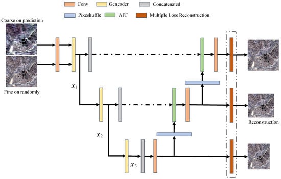
Figure 3.
Overall structure of the generator (, , represent different scale features, respectively).
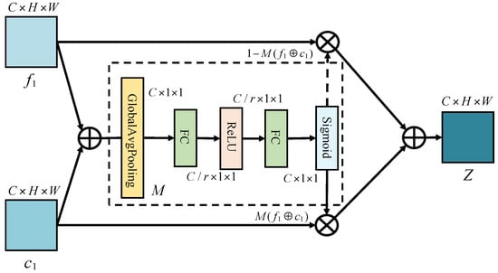
Figure 4.
Structural diagram of AFF fusion module. and are two input features, are represent the channel, height and width of the image, indicates the weight obtained by the channel focus module, ⊕ means that the elements are added directly, ⊗ means that the elements are multiplied.
The generator consists of two building blocks: an encoder and a decoder. The encoder mainly extracts standard high-pass features over the main branch, and the decoder restores the original data while recovering the data for dimensionality reduction processing. In the structure of this generator, we mainly describe the encoder. As shown in Figure 5a, an arbitrary fine-resolution image is input through the main branch. The coarse resolution of the prediction time is input through the horizontal branch, generating fine intermediate features. From Figure 5a, it can be seen that the principal component consists of a switchable normalization [56] and leaky recognized linear unit (LeakyReLU) [57] function with two cycles. In the middle, a convolution operation with a step size of 2 and a convolutional kernel size of is performed to reduce the feature size. In the horizontal branch, we use convolution operations twice to obtain coarser spectral information, and add a flexible CBAM module to adaptively rescale the spatial and channel features without increasing computational complexity to enhance the salient regions and extract more detailed features. In the concatenated block used in the generator decoder (as shown in Figure 5b), we use a convolution operation in the horizontal branch, mainly to adjust the channel of feature mapping to match the balanced output. At the end of the encoder, we match the extracted fine, coarse, abstract, and multi-level features and merge them with the decoder. In the whole generator, we use switchable normalization (SN) from feature extraction to fusion. There are four reasons for selecting SN. First, switchable normalization is a learnable normalization method driven by task and data, which can learn different normalization layers of deep neural network; Second, SN is an end-to-end learning method. It can learn important weights in the network and switch at will; Third, SN uses three different ranges to calculate statistics (mean and variance), including channel, layer and small batch. It is robust for various batch sizes and can maintain high performance even in the case of small batches. Third, SN has no sensitive hyper-parameters, and the whole network is lightweight. At the same time, after normalization, we use the leaky corrected linear unit (LeakyReLU) function to ensure that the weight is updated and maintained throughout the network propagation process. Formula (5) indicates that switchable normalization normalizes the detailed features of the reference image in phase i, Formula (6) indicates that the end-to-end PixelShuffler module is used to upsample the spatiotemporal features in phase i and , and Formula (7) indicates that the multi-level features obtained in phase i and are fused. Feature fusion throughout the generator can be expressed as follows:
wherein, represents the detail features of the reference image at stage i, and represents the spatio-temporal feature mapping after the output of stage .
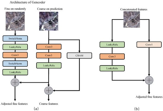
Figure 5.
(a,b) Encoder structure diagram in generator structure. CBAM represents convolution block attention module, Conv3 represents convolution operations twice to obtain coarser spectral information, Conv1 represents convolution operation in the horizontal branch, mainly to adjust the channel of feature mapping to match the balanced output.
3.4. Discriminator
The discriminator refers to the GAN-STFM model [18] and is a binary classifier consisting of resnet residual blocks (D-resBlocks). As shown in Figure 6, the first input of the discriminator is a pair of coarse images and at prediction time or a prediction image. Since we want to reduce the dependence of the whole model input image on the time series, we use the coarse image of the prediction time as the primary training data set in the training process. Second, as shown in Figure 6b, we use the main branch and transverse branch in each D-resBlocks, and use spectral normalization to stabilize the whole confrontation process. Finally, the conditional input of the discriminator is downscaled to different scales, the coefficients are set to and , and a multi-scale discriminator is used to quickly improve the initial image.
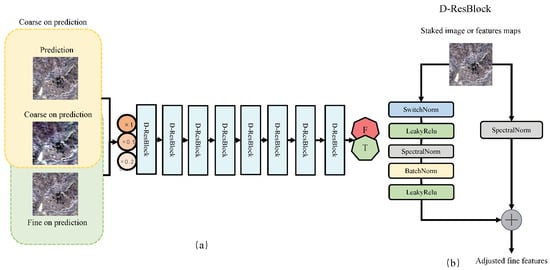
Figure 6.
Structure diagram of the Discriminator model. ((a) in the figure shows the overall structure diagram of the discriminator, in which the input of the original discriminator is sampled at three levels with factors of 1, 0.5, and 0.25 to train the multi-scale discriminator. D-ResBlock is the residual block used in the discriminator. The details of these basic building blocks are shown in Figure (b). The input of the original discriminator is sampled at three levels with a factor of 1, 0.5, and 0.25 to train the multi-scale discriminator).
3.5. Convolutional Block Attention Module
The actual convolutional operation extracts features by mixing cross-channel and spatial information. Therefore, we introduce the convolutional block attention module (CBAM), a flexible module. The detailed module structure is shown in Figure 7. The core idea of this module is to focus on the “what” and the “where” of the channel and spatial axis, respectively, and to enhance the meaningful features of the channel and spatial axis dimensions by sequentially applying the channel and spatial attention modules. The computational cost is almost negligible [20]. In this paper, the CBAM module is added to the model generator, which is mainly used to extract more detailed features and improve the representation ability of the convolutional network. Secondly, CBAM can maintain the balance and stability of the network during the game between the two networks (note that the CBAM module added to the generator is not applied to the last convolutional layer of the generator, because the generator generates images after the last convolutional layer.). The specific focus process of CBAM is shown in Formulas (8) and (9):
Given an intermediate feature map as input , CBAM successively derives a one-dimensional channel map and two-dimensional spatial map , and is the final refined output.
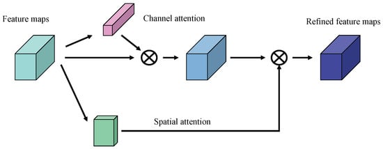
Figure 7.
The CBAM module is structured as follows.
3.6. Multiple Loss Function
In this model, the idea of multiple loss is adopted. The loss of the image itself includes feature loss (), spectral angle loss (), and visual loss () [44]. In each scale extraction process, the loss is calculated once and added in the reconstruction phase. Therefore, the total loss in this paper is defined as follows.
where , , , and are the weighting coefficients. detects perceptual differences and generates high-quality images. It can be computed using an associated automatic encoder that reduces the differences of an abstract high feature level. is shown in Formula (12). Cosine similarity is used to reduce and control the spectral distortion between different wavebands. is used to retain more detailed ground texture from the computer vision of view and provide an intuitive effect to the user.
4. Experiment and Result Analysis
4.1. Datasets, Experiment Setup and Evaluation Indicators
In this paper, we use two open-source datasets, namely, the Coleambally Irrigation Area (CIA) dataset and the lower Gwydir catchments (LGC) [58], to test the effectiveness of this model. The main characteristics of the CIA dataset are as follows: The dataset includes 17 pairs of cloud-free Landsat MODIS image pairs, with a date range from October 2001 to May 2002. The primary image type is the summer crop acreage image dataset. Over time, the phenological image features in the dataset become apparent, and the image size is . The main features of the LGC dataset are: The dataset contains 14 pairs of MODIS Landsat images. Since the site was hit by a flood disaster in 2004, the spatiotemporal features are obvious. The date range is from April 2004 to April 2005, and the image size is .
The experimental idea of this paper is to perform ablation experiments according to the MCBAM-GAN model and to check the robustness of our model by gradually increasing multi-scale, CBAM and multi-scale CBAM with respect to the original model. Second, the feasibility of this model compared with the classical model comparison algorithm is demonstrated by quantitative analysis. Finally, the model in this paper is analyzed in detail by the qualitative evaluation of the local area of the image and the thermal dispersion diagram. In the implementation of the model, we use the Python programming language to develop the PyTorch framework based on deep learning. For training, the model uses the Adam optimization method to update the model parameters. The initial learning rate is set to and the batch size is set to 8. In the training process, we input a pair of reference and predicted images. Considering the large memory requirement of the computer, we train the images in blocks. The size of the cropped images is CIA and LGC . Our whole model uses of the dataset for training, for verification, and for testing to prove the fusion and reconstruction ability of the model.
In this paper, six comprehensive indicators are used for quantitative evaluation methods. They are peak signal-to-noise ratio (PSNR), structural similarity (SSIM), spectral angle mapper (SAM), relative dimensionless global error in synthesis (ERGAS), and spatial correlation coefficient (CC), root mean square error (RMSE) [1]. The closer the SSIM value, the higher the similarity between the two images. A smaller RMSE and ERGAS represent better fusion results.
4.2. Ablation Experiments
In this paper, some ablation experiments are performed on the model to discuss the improvement effect of multi-scale, convolutional block attention modules, multiple loss functions, etc. on the overall spatiotemporal fusion model and network performance.
4.2.1. Multi Scale Ablation Experiments on LGC and CIA Datasets
The MCBAM model in this paper is a generator discriminator structure. In the U-NET network structure of the generator, we add multi-scale ideas, CBAM modules and other structures to extract the temporal, spatial and spectral features of the image in a multidimensional way. Multiple loss calculation is performed in each scale to provide a good basis for the final reconstruction and loss addition.
Previous spatio-temporal fusion models based on deep learning focus on extracting temporal and spatial features and neglect the details of texture features. The idea of the multi-scale model is to introduce images of different sizes into the downsampling process and perceive the images of different scales to improve the universality of the network. At the same time, as the depth of the network increases and the size of the receptive field increases, a multi-scale idea is developed to process and preserve large-scale semantic features to extract richer texture features. In Table 2, 1 represents one scale, 2 represents two scales, and 3 represents three scales. To achieve the expected effect and to account for model parameters and efficiency, we use only three scales. The results in Table 2 show that the multi-scale and multi-stage fusion effectively improve the prediction accuracy. The PSNR and SSIM evaluation indicators for the CIA and LGC datasets show significant improvement.
Table 2.
Quantitative Results of Multiscale on CIA and LGC Datasets.
4.2.2. Adding Ablation Experiments of Different Modules to LGC and CIA Datasets
This ablation experiment is used to add and test different modules to different datasets. This model mainly consists of six modules: (1) multi-scale module only; (2) CBAM module only; (3) multi-scale module and CBAM module; (4) multi-scale module and AFF fusion module; (5) multi-scale module, CBAM module and AFF fusion module; (6) multi-scale module, CBAM module, AFF fusion module, and multiple loss. For details, see Table 3 and Table 4.
Table 3.
Ablation experiments on CIA dataset.
Table 4.
Ablation experiments on LGC dataset.
From Table 3 and Table 4, we can see that the more modules we gradually add to the model, the better the network model works. This is because each module plays a crucial role in feature extraction, feature fusion, and reconstruction. From the table, we can also see that the performance of the CBAM module alone is better when only multi-scale modules are used, and the model parameters are almost the same. The result of using multi-scale and CBAM modules simultaneously is better than that of using CBAM and multi-scale modules alone. This is because the CBAM module extracts features from the mixture of channel and spatial information to obtain more helpful information and produce high-quality images. By gradually increasing the modules, the overall evaluation indicators of our model are better than those of the individual modules, which shows that the final generation of high-quality images is closely related to each stage of feature extraction, feature fusion, and multi-scale reconstruction. The running time of our model on the LGC dataset is higher than on the CIA dataset because the image size of the LGC dataset is 3200 × 2720, which proves that differences in data size lead to differences in time.
4.3. Detailed Analysis of the Model on the CIA Dataset
4.3.1. Quantitative Results Analysis on CIA Dataset
To prove the validity of the MCBAM-GAN model proposed in this paper, we selected five methods, STARFM [25], FSDAF [38], DCSTFN [43], DCSTFN [44], and GANSTFM [18], for comparison with the dataset CIA. STARFM and FSDAF are both traditional methods with good performance. EDCSTFN and GANSTFM are classical methods based on deep learning, EDCSTFN is a framework using CNN, and GANSTFM uses the architecture of GANs. The specific quantitative analysis is shown in Table 5.
Table 5.
Compares MCBAM-GAN with some of the most advanced models in the CIA dataset. The values in bold are the best results.
As shown in Table 5, six common evaluation indicators are selected from an objective perspective to compare and evaluate our proposed model and the classical model. The final results show that our proposed spatio-temporal fusion model achieves the optimal values of global indicators and most local indicators. We compare the deep learning based CNN structure model with deep learning based GAN structure model, and our model shows good performance. Firstly, we owe this to the powerful model performance of confrontation network generation and the ability to generate more explicit and authentic samples. Secondly, our model adds a CBAM module to extract more detailed features while reducing the input of image pairs. Finally, we add the concept of multi-scale sampling in the process of generating the U-NET structure, extract features of different scales at each stage and perform multiple loss operations to provide sufficient conditions for the final reconstruction. At the same time, we can see that our model has an advantage in terms of time consumption, since our model reduces the number of network layers and thus shortens the runtime of the model.
4.3.2. Qualitative Result Analysis on CIA Dataset
To visually represent our experimental results. Figure 8, Figure 9 and Figure 10 show the comparison results of FSDAF [25], STARFM [38], DCSTFN [43], EDCSTFN [44], GANSTFM [18] and the MCBAM-GAN model proposed in this paper for the dataset CIA.
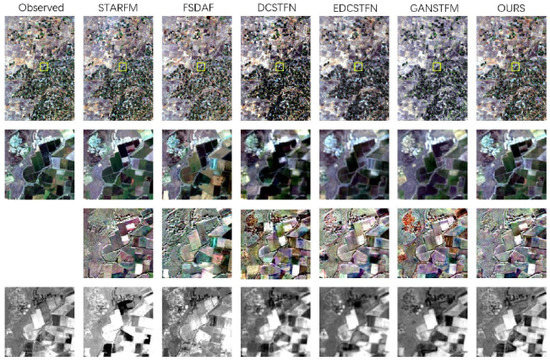
Figure 8.
Show the results in a partial enlargement of the CIA dataset. (Each column in the figure represents the predicted image of each model, “OURS” represents the MCBAM-GAN model, and “observed” represents the actual label.)
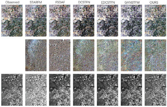
Figure 9.
The global rendering result of the CIA dataset.
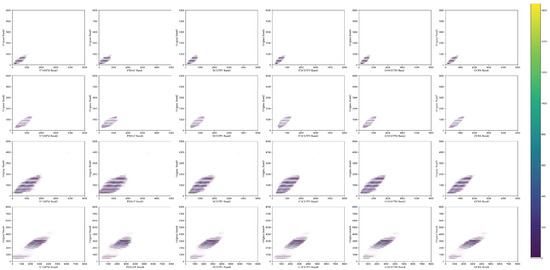
Figure 10.
Thermal scattering results for the CIA dataset. (Each column corresponds to the comparison of each band. The abscissa is the band of the predicted image, and the ordinate is the band of the real image.)
Figure 8 shows the local experimental results we obtained with the CIA dataset. We have extracted some prediction results for display. Below that, “Observed” represents the actual observed image, the first line represents the predicted image of the model, the second line represents the difference between the predicted result and the actual observed value, the third line represents the normalized vegetation index (NDVI) of the predicted value, and “Our” represents our MCBAM-GAN method. From the overall effect picture, it can be seen that our proposed method has excellent visual experience, and the definition is much closer to the original image. Figure 8 shows almost the same model image and the actual image. We have added multi-scale ideas at each stage of feature extraction, feature fusion, and reconstruction. We also extracted coarse, fine, and spatio-temporal features of different dimensions. However, from the perspective of the spectrum, the traditional methods are more advantageous. To achieve a subjective evaluation effect, we extracted and enlarged some areas, as shown in Figure 9. The first line represents the prediction results of each model, the second line represents the magnified representation of the yellow box, the third line represents the difference between the magnified area and the actual observed value, and the fourth line represents the NDVI of the magnified area. From the figure, it can be seen that the areas with dense STARFM and FSDAF features are the reason why traditional methods focus only on temporal and spatial features and ignore the details of texture features. The methods based on deep learning, such as EDCSTFN and GANSTFM, can not only predict dense areas but also clearly identify the differences between different color areas and predict farmland, roads, and other information more accurately. However, the results show that the effect on irregular areas could be better. The reason is that the CIA dataset mainly contains crop phenology dataset, including many farmland planting and irrigation areas. Figure 10 compares the thermal scatter plots of the predicted results of each model in the CIA dataset. In Figure 10, each row represents different models. A total of six models are shown in the figure. Each column represents the thermal scattering diagram of each model in four bands. The thermal scatter graph is mainly used to locate and count targets. It can be seen that the “point cloud” of our method is sparse in each band, indicating that the prediction results of our method are closer to the actual observated values and also indicating that our method is more robust in dealing with complex changes.
4.4. Detailed Analysis of the Model on the LGC Dataset
4.4.1. Quantitative Analysis of the Model on the LGC Dataset
Similarly, we will compare and analyze the MCBAM-GAN temporal-spatial fusion models and FSDAF [25], STARFM [38], EDCSTFN [44], and GANSTFM [18] with the LGC dataset. Since the LGC dataset was acquired in 2004, the collected image contains the temporal and spatial features of the image which are more obvious and have a wide range of spectral information changes. As a result, the LGC dataset has good advantages in quantitative and qualitative analysis. The transmitted quantitative analysis is shown in Table 6.
Table 6.
Compares MCBAM-GAN in LGC datasets with some of the most advanced models. The value of the thick body is the best result.
It can be seen from Table 6 that the overall evaluation indicators of our model are better than those of the other five classical models. We believe that the reason for this is twofold: First, the input of images is lower than other models and the selection of reference images is not subject to several constraints, which increases the flexibility of the model. Second, we use the U-NET and the CBAM module in the generator to increase the balance of the network and make the network run more stable. Among others, PSNR and SSIM are significantly improved, which makes the final generated image closer to the original image in terms of visual experience. It should be noted that our model is superior to the other models in terms of performance and parameters. This is because we reduce the number of network layers, ensure performance and save computer resources.
4.4.2. Qualitative Analysis of Models on LGC Datasets
Figure 11 and Figure 12 show the visual impact of each model on the LGC dataset. From the results in Figure 11, it can be seen that the output image of the STARFM model contains too much noise, which can be considered as the reason that the model is an earlier spatio-temporal fusion algorithm, that lacks the detection regional boundary space features such as rivers and roads. However, the model is good at processing spectral information. From the output image of the FSDAF model, it can be seen that the deviation to the region is striking because the algorithm cannot adapt to the dynamic features and repeatedly splits the invariant pixels. The deep learning based on algorithm has obvious errors for dark areas because the deep learning based on model largely depends on the learning experience. It can also be seen from the figure that the overall statistical features of the prediction time of the proposed model fusion image are more similar to the actual image, which means that the overall difference is negligible. This is due to the fact that the model complements the ideas of multi-scale and CBAM to fully extract multi-level features. As for the NDVI value, our model is closer to the actual value. From Table 6, PSNR and SSIM of our model are significantly higher than those of other models, indicating that our model extracts more structural information and texture details. Figure 13 compares the plots of the thermal of the predicted results of each model in the LGC dataset. From the figure, it can be seen that the “point cloud” density of all models is high, which we believe is a feature of the LGC dataset. Our model has a higher density, which indicates that the image resolution is improved in the reconstruction stage, which may facilitate target detection in the final remote sensing images.
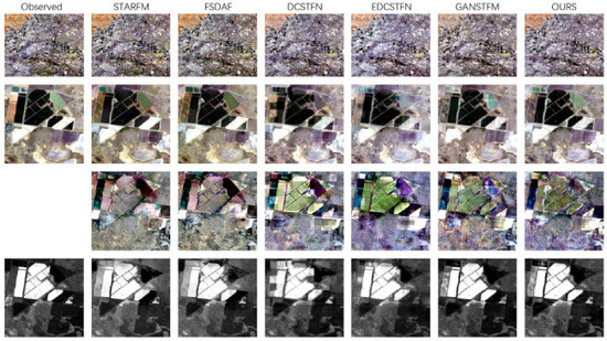
Figure 11.
Local magnification of the LGC dataset shows the results.
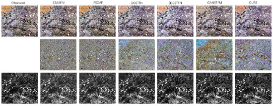
Figure 12.
Global rendering result of the LGC dataset.
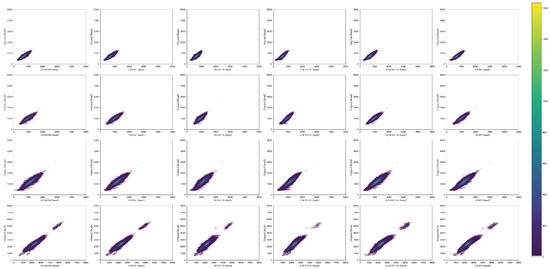
Figure 13.
The results are shown in the thermal scatter plot of the LGC dataset.
5. Conclusions
This paper proposes a spatiotemporal fusion model MCBAM-GAN based on multi-scale and CBAM convolutional attention. The proposed model consists of a generator discriminator. The generator backbone network is a U-NET network divided into three stages: multi-feature extraction, feature fusion, and image reconstruction. The idea of multi-scale and CBAM is introduced into the generator. First, the features are extracted at different levels by different scales. Then, the CBAM module enhances meaningful features in channel and spatial axis dimensions by sequentially applying channel and spatial attention modules with negligible computational load to prepare the later fusion. We use the AFF fusion module to replace the previous channel cascade method in the fusion phase. Finally, image reconstruction is performed using multiple loss functions to comprehensively consider the reconstruction of image features, vision and other aspects. In the experimental part, we performed quantitative and qualitative analyzes using ablation experiments and the classical SSTARFM, FSDAF, EDCSTFN, and GAN-STFM models. The results showed that our proposed model is more robust. Spatiotemporal fusion is always a difficult problem in super-resolution remote sensing reconstruction. Next, we will study it from two aspects. First, we will develop and propose a lightweight and universal model from the model perspective to reduce the constraints of the model to the input image. Second, we will analyze the unique attributes of each data set and investigate each kind of dataset that can finally be applied to the actual scene.
Author Contributions
Conceptualization, H.L. and Y.Q.; methodology, H.L.; software, H.L., and G.Y.; validation, H.L., G.Y. and F.D.; formal analysis, H.L.; investigation, H.L. and G.Y.; resources, Y.Q.; data curation, H.L. and Y.F.; writing—original draft preparation, H.L.; writing—review and editing, F.D.; visualization, H.L. and G.Y.; supervision, Y.Q.; project administration, H.L.; funding acquisition, Y.Q. All authors have read and agreed to the published version of the manuscript.
Funding
This work was supported by the National Natural Science Foundation of China (61966035, 62266043), the National Science Foundation of China under Grant (U1803261), the Natural Science Foundation of the XinJiang Uygur Autonomous Region (2021D01C077), the Autonomous Region Graduate Innovation Project (XJ2019G069, XJ2021G062 and XJ2020G074).
Data Availability Statement
Data sharing is not applicable to this article.
Acknowledgments
The authors would like to thank all of the reviewers for their valuable contributions to our work.
Conflicts of Interest
The authors declare no conflict of interest.
Abbreviations
The following abbreviations are used in this manuscript:
| HTHS | high-temporal and high-spatial |
| CBAM | convolutional block attention module |
| MCBAM | multiscale and convolutional block attention module |
| MODIS | moderate-resolution imaging spectroradiometer |
| CNN | convolutional neural network |
| GAN | generative adversarial network |
| CIA | coleambally irrigation area |
| LGC | lower gwydir catchments |
| STARFM | spatio-temporal adaptive reflection fusion model |
| FSDAF | flexible spatio-temporal data fusion |
| SPSTFM | spatiotemporal reflectance fusion model |
| STFDCNN | spatiotemporal fusion algorithm based on CNN |
| DCSTFN | depth convolution spatiotemporal fusion network |
| BiaSTF | bias-driven spatio-temporal fusion models |
| SSTSTF | spatial, sensor, and temporal spatio-temporal fusion |
| LSGAN | least squares GAN |
| ResNet | residual network |
| AFF | attention feature fusion |
| LeakyReLU | leaky recognized linear unit |
| PSNR | peak signal-to-noise ratio |
| SSIM | structural similarity |
| SAM | spectral angle mapper |
| ERGAS | relative dimensionless global error in synthesis |
| CC | spatial correlation coefficient |
| RMSE | root mean square error |
| NDVI | normalized vegetation index |
References
- Liu, H.; Qian, Y.; Zhong, X.; Chen, L.; Yang, G. Research on super-resolution reconstruction of remote sensing images: A comprehensive review. Opt. Eng. 2021, 60, 100901. [Google Scholar] [CrossRef]
- Li, W.; Zhang, X.; Peng, Y.; Dong, M. Spatiotemporal fusion of remote sensing images using a convolutional neural network with attention and multiscale mechanisms. Int. J. Remote Sens. 2021, 42, 1973–1993. [Google Scholar] [CrossRef]
- Walker, J.; Beurs, K.D.; Wynne, R.; Gao, F. Evaluation of Landsat and MODIS data fusion products for analysis of dryland forest phenology. Remote Sens. Environ. 2012, 117, 381–393. [Google Scholar] [CrossRef]
- Cheng, G.; Yang, C.; Yao, X.; Guo, L.; Han, J. When Deep Learning Meets Metric Learning: Remote Sensing Image Scene Classification via Learning Discriminative CNNs. IEEE Trans. Geosci. Remote Sens. 2018, 56, 2811–2821. [Google Scholar] [CrossRef]
- Yao, X.; Feng, X.; Han, J.; Cheng, G.; Guo, L. Automatic Weakly Supervised Object Detection from High Spatial Resolution Remote Sensing Images via Dynamic Curriculum Learning. IEEE Trans. Geosci. Remote Sens. 2021, 59, 675–685. [Google Scholar] [CrossRef]
- Hong, D.; Yao, J.; Meng, D.; Xu, Z.; Chanussot, J. Multimodal GANs: Toward Crossmodal Hyperspectral-Multispectral Image Segmentation. IEEE Trans. Geosci. Remote Sens. 2021, 59, 5103–5113. [Google Scholar] [CrossRef]
- Lees, K.; Quaife, T.; Artz, R.; Khomik, M.; Clark, J. Potential for using remote sensing to estimate carbon fluxes across northern peatlands—A review. Sci. Total. Environ. 2018, 615, 857–874. [Google Scholar] [CrossRef]
- Galford, G.L.; Mustard, J.F.; Melillo, J.; Gendrin, A.; Cerri, C.C.; Cerri, C.E. Wavelet analysis of MODIS time series to detect expansion and intensification of row-crop agriculture in Brazil. Remote Sens. Environ. 2008, 112, 576–587. [Google Scholar] [CrossRef]
- Deng, M.; Di, L.; Han, W.; Yagci, A.L.; Peng, C.; Heo, G. Web-service-based monitoring and analysis of global agricultural drought. Photogramm. Eng. Remote Sens. 2013, 79, 929–943. [Google Scholar] [CrossRef]
- Li, J.; Li, Y.; He, L.; Chen, J.; Plaza, A. Spatio-temporal fusion for remote sensing data: An overview and new benchmark. Sci. China Inf. Sci. 2020, 63, 140301. [Google Scholar] [CrossRef]
- Roy, D.P.; Wulder, M.A.; Loveland, T.R.; Woodcock, C.E.; Allen, R.G.; Anderson, M.C.; Helder, D.; Irons, J.R.; Johnson, D.M.; Kennedy, R.; et al. Landsat-8: Science and product vision for terrestrial global change research. Remote Sens. Environ. 2014, 145, 154–172. [Google Scholar] [CrossRef]
- Justice, C.; Vermote, E.F.; Townshend, J.R.; DeFries, R.S.; Roy, D.P.; Hall, D.K.; Salomonson, V.V.; Privette, J.L.; Riggs, G.A.; Strahler, A.H.; et al. The Moderate Resolution Imaging Spectroradiometer (MODIS): Land remote sensing for global change research. IEEE Trans. Geosci. Remote Sens. 1998, 36, 1228–1249. [Google Scholar] [CrossRef]
- Goodfellow, I.J.; Pouget-Abadie, J.; Mirza, M.; Xu, B.; Warde-Farley, D.; Ozair, S.; Courville, A.C.; Bengio, Y. Generative Adversarial Nets. In Proceedings of the Advances in Neural Information Processing Systems 27: Annual Conference on Neural Information Processing Systems 2014, Montreal, QC, Canada, 8–13 December 2014; pp. 2672–2680. [Google Scholar]
- Zhu, J.; Krähenbühl, P.; Shechtman, E.; Efros, A.A. Generative Visual Manipulation on the Natural Image Manifold. In Proceedings of the Computer Vision—ECCV 2016—14th European Conference, Amsterdam, The Netherlands, 11–14 October 2016; Volume 9909, pp. 597–613. [Google Scholar]
- Liu, G.; Reda, F.A.; Shih, K.J.; Wang, T.; Tao, A.; Catanzaro, B. Image Inpainting for Irregular Holes Using Partial Convolutions. In Proceedings of the Computer Vision—ECCV 2018—15th European Conference, Munich, Germany, 8–14 September 2018; Volume 11215, pp. 89–105. [Google Scholar]
- Ledig, C.; Theis, L.; Huszar, F.; Caballero, J.; Cunningham, A.; Acosta, A.; Aitken, A.P.; Tejani, A.; Totz, J.; Wang, Z.; et al. Photo-Realistic Single Image Super-Resolution Using a Generative Adversarial Network. In Proceedings of the 2017 IEEE Conference on Computer Vision and Pattern Recognition, CVPR 2017, Honolulu, HI, USA, 21–26 July 2017; pp. 105–114. [Google Scholar]
- Zhang, H.; Song, Y.; Han, C.; Zhang, L. Remote Sensing Image Spatiotemporal Fusion Using a Generative Adversarial Network. IEEE Trans. Geosci. Remote Sens. 2021, 59, 4273–4286. [Google Scholar] [CrossRef]
- Tan, Z.; Gao, M.; Li, X.; Jiang, L. A Flexible Reference-Insensitive Spatiotemporal Fusion Model for Remote Sensing Images Using Conditional Generative Adversarial Network. IEEE Trans. Geosci. Remote Sens. 2022, 60, 5601413. [Google Scholar] [CrossRef]
- Chen, J.; Wang, L.; Feng, R.; Liu, P.; Han, W.; Chen, X. CycleGAN-STF: Spatiotemporal Fusion via CycleGAN-Based Image Generation. IEEE Trans. Geosci. Remote Sens. 2021, 59, 5851–5865. [Google Scholar] [CrossRef]
- Arjovsky, M.; Chintala, S.; Bottou, L. Wasserstein Generative Adversarial Networks. In Proceedings of the 34th International Conference on Machine Learning, ICML 2017, Sydney, NSW, Australia, 6–11 August 2017; Volume 70, pp. 214–223. [Google Scholar]
- Zhukov, B.; Oertel, D.; Lanzl, F.; Reinhäckel, G. Unmixing-based multisensor multiresolution image fusion. IEEE Trans. Geosci. Remote Sens. 1999, 37, 1212–1226. [Google Scholar] [CrossRef]
- Wu, M.; Niu, Z.; Wang, C.; Wu, C.; Wang, L. Use of MODIS and Landsat time series data to generate high-resolution temporal synthetic Landsat data using a spatial and temporal reflectance fusion model. J. Appl. Remote Sens. 2012, 6, 063507. [Google Scholar]
- Zhang, W.; Li, A.; Jin, H.; Bian, J.; Zhang, Z.; Lei, G.; Qin, Z.; Huang, C. An Enhanced Spatial and Temporal Data Fusion Model for Fusing Landsat and MODIS Surface Reflectance to Generate High Temporal Landsat-Like Data. Remote Sens. 2013, 5, 5346–5368. [Google Scholar] [CrossRef]
- Lu, M.; Chen, J.; Tang, H.; Rao, Y.; Yang, P.; Wu, W. Land cover change detection by integrating object-based data blending model of Landsat and MODIS. Remote Sens. Environ. 2016, 184, 374–386. [Google Scholar] [CrossRef]
- Gao, F.; Masek, J.G.; Schwaller, M.R.; Hall, F.G. On the blending of the Landsat and MODIS surface reflectance: Predicting daily Landsat surface reflectance. IEEE Trans. Geosci. Remote Sens. 2006, 44, 2207–2218. [Google Scholar]
- Zhu, X.; Chen, J.; Gao, F.; Chen, X.; Masek, J.G. An enhanced spatial and temporal adaptive reflectance fusion model for complex heterogeneous regions. Remote Sens. Environ. 2010, 114, 2610–2623. [Google Scholar] [CrossRef]
- Hilker, T.; Wulder, M.A.; Coops, N.C.; Linke, J.; McDermid, G.; Masek, J.G.; Gao, F.; White, J.C. A new data fusion model for high spatial-and temporal-resolution mapping of forest disturbance based on Landsat and MODIS. Remote Sens. Environ. 2009, 113, 1613–1627. [Google Scholar] [CrossRef]
- Weng, Q.; Fu, P.; Gao, F. Generating daily land surface temperature at Landsat resolution by fusing Landsat and MODIS data. Remote Sens. Environ. 2014, 145, 55–67. [Google Scholar] [CrossRef]
- Li, A.; Bo, Y.; Zhu, Y.; Guo, P.; Bi, J.; He, Y. Blending multi-resolution satellite sea surface temperature (SST) products using Bayesian maximum entropy method. Remote Sens. Environ. 2013, 135, 52–63. [Google Scholar] [CrossRef]
- Liao, L.; Song, J.; Wang, J.; Xiao, Z.; Wang, J. Bayesian Method for Building Frequent Landsat-Like NDVI Datasets by Integrating MODIS and Landsat NDVI. Remote Sens. 2016, 8, 452. [Google Scholar] [CrossRef]
- Shen, H.; Meng, X.; Zhang, L. An Integrated Framework for the Spatio-Temporal-Spectral Fusion of Remote Sensing Images. IEEE Trans. Geosci. Remote Sens. 2016, 54, 7135–7148. [Google Scholar] [CrossRef]
- Xue, J.; Leung, Y.; Fung, T. A Bayesian Data Fusion Approach to Spatio-Temporal Fusion of Remotely Sensed Images. Remote Sens. 2017, 9, 1310. [Google Scholar] [CrossRef]
- Huang, B.; Song, H. Spatiotemporal Reflectance Fusion via Sparse Representation. IEEE Trans. Geosci. Remote Sens. 2012, 50, 3707–3716. [Google Scholar] [CrossRef]
- Song, H.; Huang, B. Spatiotemporal Satellite Image Fusion Through One-Pair Image Learning. IEEE Trans. Geosci. Remote Sens. 2013, 51, 1883–1896. [Google Scholar] [CrossRef]
- Wu, B.; Huang, B.; Zhang, L. An Error-Bound-Regularized Sparse Coding for Spatiotemporal Reflectance Fusion. IEEE Trans. Geosci. Remote Sens. 2015, 53, 6791–6803. [Google Scholar] [CrossRef]
- Gevaert, C.M.; García-Haro, F.J. A comparison of STARFM and an unmixing-based algorithm for Landsat and MODIS data fusion. Remote Sens. Environ. 2015, 156, 34–44. [Google Scholar] [CrossRef]
- Li, X.; Ling, F.; Foody, G.M.; Ge, Y.; Zhang, Y.; Du, Y. Generating a series of fine spatial and temporal resolution land cover maps by fusing coarse spatial resolution remotely sensed images and fine spatial resolution land cover maps. Remote Sens. Environ. 2017, 196, 293–311. [Google Scholar] [CrossRef]
- Zhu, X.; Helmer, E.H.; Gao, F.; Liu, D.; Chen, J.; Lefsky, M.A. A flexible spatiotemporal method for fusing satellite images with different resolutions. Remote Sens. Environ. 2016, 172, 165–177. [Google Scholar] [CrossRef]
- Li, X.; Foody, G.M.; Boyd, D.S.; Ge, Y.; Zhang, Y.; Du, Y.; Ling, F. SFSDAF: An enhanced FSDAF that incorporates sub-pixel class fraction change information for spatio-temporal image fusion. Remote Sens. Environ. 2020, 237, 111537. [Google Scholar] [CrossRef]
- Guo, D.; Shi, W.; Hao, M.; Zhu, X. FSDAF 2.0: Improving the performance of retrieving land cover changes and preserving spatial details. Remote Sens. Environ. 2020, 248, 111973. [Google Scholar] [CrossRef]
- Ma, Y.; Wang, L.; Liu, P.; Ranjan, R. Towards building a data-intensive index for big data computing—A case study of Remote Sensing data processing. Inf. Sci. 2015, 319, 171–188. [Google Scholar] [CrossRef]
- Song, H.; Liu, Q.; Wang, G.; Hang, R.; Huang, B. Spatiotemporal Satellite Image Fusion Using Deep Convolutional Neural Networks. IEEE J. Sel. Top. Appl. Earth Obs. Remote Sens. 2018, 11, 821–829. [Google Scholar] [CrossRef]
- Tan, Z.; Yue, P.; Di, L.; Tang, J. Deriving High Spatiotemporal Remote Sensing Images Using Deep Convolutional Network. Remote Sens. 2018, 10, 1066. [Google Scholar] [CrossRef]
- Tan, Z.; Di, L.; Zhang, M.; Guo, L.; Gao, M. An Enhanced Deep Convolutional Model for Spatiotemporal Image Fusion. Remote Sens. 2019, 11, 2898. [Google Scholar] [CrossRef]
- Liu, X.; Deng, C.; Chanussot, J.; Hong, D.; Zhao, B. StfNet: A Two-Stream Convolutional Neural Network for Spatiotemporal Image Fusion. IEEE Trans. Geosci. Remote Sens. 2019, 57, 6552–6564. [Google Scholar] [CrossRef]
- Li, Y.; Li, J.; He, L.; Chen, J.; Plaza, A. A new sensor bias-driven spatio-temporal fusion model based on convolutional neural networks. Sci. China Inf. Sci. 2020, 63, 140302. [Google Scholar] [CrossRef]
- Ma, Y.; Wei, J.; Tang, W.; Tang, R. Explicit and stepwise models for spatiotemporal fusion of remote sensing images with deep neural networks. Int. J. Appl. Earth Obs. Geoinf. 2021, 105, 102611. [Google Scholar] [CrossRef]
- Wang, X.; Wang, X. Spatiotemporal Fusion of Remote Sensing Image Based on Deep Learning. J. Sens. 2020, 2020, 8873079:1–8873079:11. [Google Scholar] [CrossRef]
- Li, W.; Zhang, X.; Peng, Y.; Dong, M. DMNet: A network architecture using dilated convolution and multiscale mechanisms for spatiotemporal fusion of remote sensing images. IEEE Sens. J. 2020, 20, 12190–12202. [Google Scholar] [CrossRef]
- Peng, M.; Zhang, L.; Sun, X.; Cen, Y.; Zhao, X. A Fast Three-Dimensional Convolutional Neural Network-Based Spatiotemporal Fusion Method (STF3DCNN) Using a Spatial-Temporal-Spectral Dataset. Remote Sens. 2020, 12, 3888. [Google Scholar] [CrossRef]
- Song, B.; Liu, P.; Li, J.; Wang, L.; Zhang, L.; He, G.; Chen, L.; Liu, J. MLFF-GAN: A Multi-Level Feature Fusion with GAN for Spatiotemporal Remote Sensing Images. IEEE Trans. Geosci. Remote Sens. 2022, 60, 4410816. [Google Scholar] [CrossRef]
- He, K.; Zhang, X.; Ren, S.; Sun, J. Deep Residual Learning for Image Recognition. In Proceedings of the 2016 IEEE Conference on Computer Vision and Pattern Recognition, CVPR 2016, Las Vegas, NV, USA, 27–30 June 2016; pp. 770–778. [Google Scholar]
- Goodfellow, I.; Pouget-Abadie, J.; Mirza, M.; Xu, B.; Warde-Farley, D.; Ozair, S.; Courville, A.; Bengio, Y. Generative adversarial networks. Commun. ACM 2020, 63, 139–144. [Google Scholar] [CrossRef]
- Ronneberger, O.; Fischer, P.; Brox, T. U-Net: Convolutional Networks for Biomedical Image Segmentation. In Proceedings of the Medical Image Computing and Computer-Assisted Intervention—MICCAI 2015—18th International Conference, Munich, Germany, 5–9 October 2015; Volume 9351, pp. 234–241. [Google Scholar]
- Zhong, X.; Qian, Y.; Liu, H.; Chen, L.; Wan, Y.; Gao, L.; Qian, J.; Liu, J. Attention_FPNet: Two-Branch Remote Sensing Image Pansharpening Network Based on Attention Feature Fusion. IEEE J. Sel. Top. Appl. Earth Obs. Remote Sens. 2021, 14, 11879–11891. [Google Scholar] [CrossRef]
- Luo, P.; Ren, J.; Peng, Z.; Zhang, R.; Li, J. Differentiable Learning-to-Normalize via Switchable Normalization. In Proceedings of the 7th International Conference on Learning Representations, ICLR 2019, New Orleans, LA, USA, 6–9 May 2019. [Google Scholar]
- Nwankpa, C.; Ijomah, W.; Gachagan, A.; Marshall, S. Activation functions: Comparison of trends in practice and research for deep learning. arXiv 2018, arXiv:1811.03378. [Google Scholar]
- Emelyanova, I.V.; McVicar, T.R.; van Niel, T.G.; Li, L.T.; Dijk, A.I.V. Assessing the accuracy of blending Landsat—MODIS surface reflectances in two landscapes with contrasting spatial and temporal dynamics: A framework for algorithm selection. Remote Sens. Environ. 2013, 133, 193–209. [Google Scholar] [CrossRef]
Disclaimer/Publisher’s Note: The statements, opinions and data contained in all publications are solely those of the individual author(s) and contributor(s) and not of MDPI and/or the editor(s). MDPI and/or the editor(s) disclaim responsibility for any injury to people or property resulting from any ideas, methods, instructions or products referred to in the content. |
© 2023 by the authors. Licensee MDPI, Basel, Switzerland. This article is an open access article distributed under the terms and conditions of the Creative Commons Attribution (CC BY) license (https://creativecommons.org/licenses/by/4.0/).