Estimation of Tropical Cyclone Intensity Using Multi-Platform Remote Sensing and Deep Learning with Environmental Field Information

Abstract

Accurate tropical cyclone (TC) intensity estimation is crucial for prediction and disaster prevention. Currently, significant progress has been achieved for the application of convolutional neural networks (CNNs) in TC intensity estimation. However, many studies have overlooked the fact that the local convolution used by CNNs does not consider the global spatial relationships between pixels. Hence, they can only capture limited spatial contextual information. In addition, the special rotation invariance and symmetry structure of TC cannot be fully expressed by convolutional kernels alone. Therefore, this study proposes a new deep learning-based model for TC intensity estimation, which uses a combination of rotation equivariant convolution and Transformer to address the rotation invariance and symmetry structure of TC. Combining the two can allow capturing both local and global spatial contextual information, thereby achieving more accurate intensity estimation. Furthermore, we fused multi-platform satellite remote sensing data into the model to provide more information about the TC structure. At the same time, we integrate the physical environmental field information into the model, which can help capture the impact of these external factors on TC intensity and further improve the estimation accuracy. Finally, we use TCs from 2003 to 2015 to train our model and use 2016 and 2017 data as independent validation sets to verify our model. The overall root mean square error (RMSE) is 8.19 kt. For a subset of 482 samples (from the East Pacific and Atlantic) observed by aircraft reconnaissance, the root mean square error is 7.88 kt.

1. Introduction

Tropical cyclones (TCs) are catastrophic weather phenomena that can significantly impact human life. The strong winds and heavy rainfall that accompany these systems can cause substantial damage to property and hinder social and economic development in the affected regions. Therefore, accurately estimating the intensity of TC is of great significance for both theoretical research and practical applications.

The most widely used method for estimating TC intensity is the Dvorak technique [1], which relates the rotation, eye shape, and thunderstorm activity of a TC to its strengthening or weakening. This technique assumes that cyclones with similar intensities often have similar patterns and requires expert analysis of visible and infrared satellite images of the TC’s cloud structures. Once relevant patterns are detected, the technique further analyzes cloud organization characteristics, core features, curvature radius, and rainfall rates to estimate the storm intensity [2,3]. As this method relies heavily on the experience of professionals, it is highly subjective. Olander et al. [4] further improved the Dvorak technique by creating a method called advanced Dvorak technique (ADT) version 9. ADT reduces subjectivity by determining the storm center, using computer-based cloud feature recognition algorithms and applying linear regression to estimate TC intensity. However, it is not suitable for estimating the intensity of weak TCs. Due to the requirement for strong vortical structures within the cyclone, the advanced Dvorak technique is not suitable for accurately estimating the intensity of weak TCs, as their weak vortical structures make accurate estimation difficult.

The deviation angle variance technique (DAVT) [5] is based on direction gradient statistical analysis of infrared satellite images to estimate the TC intensity over the North Atlantic [6] and North Pacific [7]. This method requires information about the TC center. Although the DAVT technique can automatically locate the TC center, positioning errors may lead to uncertainties in the intensity estimation.

Since the proposal of AlexNet in 2012 [8,9], deep learning algorithms have flourished. Convolutional neural networks (CNNs) consist of convolutional layers and fully connected layers, with the former extracting spatial features from input images and the latter having simple computing units. By learning to recognize features that improve the prediction of target phenomena without relying on experts in the relevant field to identify which features are the most important [10], CNNs can be applied to extract features from satellite infrared images, much like how meteorologists identify cloud patterns (e.g., hurricane eyes) associated with TCs within certain intensity ranges. These features can then be used as predictors to estimate TC intensity. Some researchers have applied CNNs for TC intensity classification. Pradhan et al. [11] proposed a deep CNN TC intensity classification model using a long time series of TC infrared cloud images, achieving an RMSE of 10.18 kt for intensity level estimation. Wimmers et al. [12] summarized the advantages of high- and low-frequency microwave bands in extracting structural information from TC, with the 85–92 GHz (89 GHz) band capturing almost all important structural information at a relatively low resolution (5 km) for the eye wall. They used a CNN model for TC intensity estimation, achieving an RMSE of 14.3 kt. Dawood et al. [13] and Combinido et al. [14] used CNN-based models as regression tasks to estimate TC intensity. However, the simplicity and directness of the regression method make it difficult for these single models to fully cover TC variability, especially when there is an imbalance in the samples of TCs of different intensities. Existing CNN-based TC intensity estimation models only focus on basic and relatively simple deep learning network structures.

Transformer is an attention-based encoder-decoder architecture and is the main deep learning model for natural language processing (NLP). Inspired by this significant achievement, some pioneering work has recently been done on applying Transformer-like structures to the field of computer vision (CV). For example, Dosovitskiy et al. [15] proposed a pure Transformer, using image patches as input for image classification and achieving outstanding performance on many image classification benchmarks. In addition, Visual Transformers have achieved excellent performance in other computer vision tasks such as detection [16], segmentation [17], tracking [18], image classification [19], and augmentation [20].

The successful application of Transformers in image recognition [21] has led us to apply Transformers to TC intensity estimation. TC intensity classification is different from that of traditional rigid objects such as cars and animals. The structure of a TC changes significantly at different development stages due to continuous rotation and translation. The features of adjacent TC intensity categories are very similar, making it difficult to distinguish between adjacent intensity categories. Additionally, TC cloud images with different cloud band structures may belong to the same intensity category. On the other hand, cloud images with similar structures may belong to two different intensity categories. For these reasons, a structurally simple CNN is insufficient to capture TC structural features. Although the convolutional kernel continuously extracts abstract high-level features, theoretically covering the entire image, many studies [22] have shown that the actual receptive field is much smaller than the theoretical receptive field, which hinders the network’s ability to fully utilize contextual information to capture TC features. The Transformer network, based on self-attention mechanisms, can capture long-range dependency relationships and global spatial relationships, and has stronger spatial context modeling capabilities. Compared to traditional CNNs, the Transformer network can capture more spatial context information, thereby improving the accuracy and generalization ability of intensity estimation. Furthermore, the self-attention mechanism of the Transformer network can help the network better understand the dependencies and differences between TCs, leading to more accurate intensity estimates.

This study proposes a model that combines rotation equivariant convolution with Transformer and incorporates environmental factors to estimate TC intensity using multi-platform remote sensing data fusion. Multi-platform remote sensing data fusion [23,24] can provide more structural features to TC. While CNN have been successful in estimating TC intensity, they have some limitations, particularly in terms of spatial context modeling. By combining convolution with Transformer networks, the limitations of using CNN alone for TC intensity estimation can be overcome. Additionally, rotation equivariant convolution can handle the rotational invariance and symmetry of TC, as they should have the same intensity regardless of their orientation. At the same time, multi-platform remote sensing satellite data fusion was used to input into the model to provide more comprehensive TC feature information. This type of convolution can detect the same features in different orientations and generate features unaffected by rotation. Finally, incorporating environmental factors such as the R35 knot wind radius (R35), sea surface temperature (SST), and TC center position can help capture the influence of external factors on TC intensity, further improving the accuracy of the estimation.

The remainder of the paper is organized as follows. Section 2 introduces the dataset and data preprocessing. Section 3 presents the methodology, and Section 4 provides the experimental setup and analysis. Section 5 presents the conclusion.

2. Data and Preprocessing

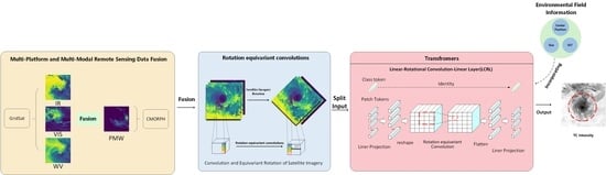
The satellite data used in this study are a fusion of multi-platform remote sensing data obtained from the publicly available Tropical Cyclone for Image-to-intensity Regression dataset (TCIR; [25]). The dataset contains satellite data from four platforms, namely infrared (IR), water vapor (WV), visible light (VIS), and passive microwave rainrate (PMW). IR, WV, and VIS data can be obtained from GridSat [26,27], which has been collecting data at a temporal resolution of 3 h and a spatial resolution of 0.07° since 1981. PMW channel data were obtained from the CMORPH [28] open source data through low-orbit microwave satellites, with a time resolution of 3 h and a spatial resolution of 0.25°. The details are shown in

Table 1. Detailed description of the four channels of the benchmark dataset.

Channel	Wavelength	Temporal Resolution (h)	Spatial Resolution (°)	Sorce	Temporal Coverage
IR	11 μm	3	0.07	GridSat	2003–2017
WV	6.7 μm	3	0.07	GridSat	2003–2017
VIS	0.6 μm	3	0.07	GridSat	2003–2017
PMW	85 Ghz	3	0.25	CMORPH	2003–2017

. To make all channels the same size, the PMW channels are rescaled to be about four times larger by linear interpolation. The IR channel contains the most useful features for TC intensity estimation, the PMW channel can address convective features under cold cloud shielding, and the WV channel can reflect the overall structure and features of TC. The VIS channel is not considered because it is only available during daylight hours. In this study, we fused three satellite remote sensing data from different platforms as input data to the model. Fusing the satellite remote sensing data from different platforms allowed for obtaining more comprehensive and specific information on TC features, which can improve the accuracy of TC intensity estimation.

The satellite remote sensing data of different platforms correspond to different depths of TC in space, and more vertical and three-dimensional atmospheric information of TC can be extracted through the fusion of satellite remote sensing data of different platforms in space, especially the structural information of the low-level atmospheric convection area. This has an important effect on the intensity, and the cloud image fusion of multi-platform remote sensing data is shown in Figure 1.

The data labels used in the study are obtained from the Joint Typhoon Warning Center [29] and the revised Atlantic hurricane database (HURDAT2). The labels are determined by experienced meteorologists from various institutions using the Dvorak method, ground observations, scatterometry, depth-based intensity estimates, objective and subjective passive microwave and infrared techniques, and SAR data in subsequent years and are continuously revised based on the entire life cycle of the TC.

We train our model using TC data from 2003 to 2014 and 2016 to avoid the influence of time-series correlation on the independent validation set. We use the Saffir–Simpson Hurricane Wind Scale (SSHWS) [11] for intensity classification (

Table 2. Saffir–Simpson Hurricane Wind Scale and associated categories.

Category	Symbol	Wind Speed (kt)
No Category	NC	≤20
Tropical depression	TD	21–33
Tropical storm	TS	34–63
One	H1	64–82
Two	H2	83–95
Three	H3	96–112
Four	H4	113–136
Five	H5	≥137

). TC data from 2003 to 2014 and 2016 are divided into training and validation datasets at a ratio of 9:1. The TC data from 2015 and 2017 are used as an independent test dataset. Reconnaissance-assisted best-track intensity in 2017 is available for TCs from the Eastern Pacific (EP) and Atlantic (AL) basins. The specific number of each dataset is shown in

Table 3. TC sample sizes for different dataset in different basins.

DataSet	Frame	Years	Basins
Training	58,447	2003–2014, 2016	Global
Validation	6495	2003–2014, 2016	Global
Testing	10,118	2015, 2017	Global
Reconnaissance assistance	482	2017	East Pacific, Atlantic

. The training dataset is used to fit the weights that best match the track intensity in the CNN model. The validation dataset is used to identify the best hyperparameters in the model. Finally, the best performance scheme determined using the validation dataset is applied to the independent test dataset for independent performance evaluation. Before training the input model, three processing steps are performed, namely center cropping, random rotation, and normalization. Random rotation relative to the TC center is used to prevent overfitting. Then, z-score normalization is applied to improve computational efficiency. Finally, the images of TCs in the southern hemisphere are horizontally flipped to train with the same TC rotation direction as in the northern hemisphere.

3. Methodology

TCICVIT is an improvement of CeiT [30], which has demonstrated good performance in intensity estimation. The CNNs use local convolutions, which do not consider the global spatial relationships between pixels. Therefore, they can only capture limited spatial context information. In contrast, Vision Transformers can process spatial and temporal information through self-attention mechanisms, allowing them to capture remote dependencies and global spatial relationships.

TC can be viewed as tropical mesoscale convective systems with rotational invariance. Rotational invariance is important for identifying arbitrarily oriented objects. Sending rotated images to conventional CNN results in different feature maps than those from the original images. Compared to traditional CNNs, group equivariant CNNs (GECNNs) [31] have stronger rotational equivariance and can better handle object recognition in any direction. This is because GECNNs extend the convolution operation from only having translational equivariance to having rotational equivariance, while CNNs can only handle translational equivariance. This extension is achieved by introducing the concept of group theory, using a group to act on the input data so that while the input data undergoes group operations, the output data can also undergo corresponding group operations, thus ensuring equivariance. Given a transformation group G and a function $\Phi$: X → Y, the equivalence can be expressed as follows.

$$\Phi \left[T_g^x\left(x\right)\right]=T_g^Y\left[\Phi \left(x\right)\right]\forall \left(x,g\right)\in \left(X,G\right)$$

(1)

where $T_g$ represents a group action in space. The CNN translational equivariance can be represented as:

$$\left[\left[T_{t}f\right]\ast \psi \right]\left(x\right)=\left[T_t\left[f\ast \psi \right]\right]\left(x\right)$$

(2)

where $T_t$ represents the action of the translation group $\left(R^2,+\right)$ in space, which we apply to a K-dimensional feature map $f:Z^2\to R^k$. The convolutional filter can be represented as $\psi$:$Z^2$→$R^k$, and ∗ denotes the convolution operation. The rotation equivariant layer is based on the cyclic group $C_N$ with discrete rotations with $\frac{2\pi }{N}$ angles. The rotation equivariant convolution can be defined as follows:

$$\left[\left[T_{g}f\right]\ast \psi \right]\left(g\right)=\left[T_g\left[f\ast \psi \right]\right]\left(g\right)$$

(3)

where g is the semidirect product of the translation and rotation groups. We improve the convolution in the CeiT model to a rotation equivariant convolution to extract TC symmetry structural features. A very important component in CeiT is the locally enhanced feed-forward layer, which promotes the correlation between adjacent tokens in the spatial dimension. We improve this component based on TC characteristics, replacing the depth-wise separable convolution with rotation equivariant convolution. The improved component plays an important role in TC intensity estimation. First, it allows the model to capture finer local features, which may be important for identifying small-scale features related to TC intensity. Secondly, it selectively focuses on different input regions to better process spatial information, which is useful for capturing the three-dimensional structure of TCs. This component is called linear–rotational convolution–linear (LRCL) in our model, and its process formula is shown as:

$$x_c^h,x_p^h=\mathrm{Split}\left(x_t^h\right)$$

(4)

$$x_p^{l_1}=\mathrm{GELU}\left(BN\left(\mathrm{Linear}1(x_p^h)\right)\right)$$

(5)

$$x_p^s=\mathrm{SpatialRestore}\left(x_p^{l_1}\right)$$

(6)

$$x_p^d=\mathrm{GELU}\left(BN\left(\mathrm{RTConv}\left(x_p^s\right)\right)\right)$$

(7)

$$x_p^f=\mathrm{Flatten}\left(x_p^d\right)$$

(8)

$$x_p^{l_2}=\mathrm{GELU}\left(BN\left(\mathrm{Linear}2(x_p^f)\right)\right)$$

(9)

$$x_t^{h+1}=\mathrm{Concat}\left(x_c^h,x_p^h\right)$$

(10)

$x_c^h$ represents the class token, $x_p^h$ denotes the patch token, $x_p^{l_1}$ indicates the patch token projected to a higher dimension, $x_p^s$ represents the patch token on the spatial dimension relative to the original image, $x_p^d$ refers to the patch token with enhanced correlation achieved by performing rotation equivariant convolution, and $x_p^f$ is the flattened sequence. $x_p^{l_2}$ is the linear projection of the patch token to the initial dimension, which is finally concatenated with the class patch token. BatchNorm and GELU are added after each linear projection and rotation equivariant convolution. BatchNorm can normalize and regularize the network, avoid the occurrence of gradient vanishing and exploding problems, accelerate network training, and improve model performance and generalization ability. Meanwhile, GELU can improve the model’s non-linear expression ability and generalization performance, adapt to deep network training, and enhance model stability and accuracy.

The training process of the model is as follows. First, features are extracted through rotation equivariant convolutions and increased in channels before being segmented into patches for vectorization. These patches are extracted from the feature maps rather than the original input image. The learned feature maps are extracted as a sequence of patches in the spatial dimension, fully utilizing the advantages of rotation equivariant convolutions in extracting low-level features while reducing the number of parameters. Secondly, the token generated by the multi-head self-attention (MSA) module is split into corresponding patch tokens and a class token. MSA can perform global information interaction and adaptive feature extraction on various meteorological elements, thereby improving the accuracy and stability of intensity estimation. The patch tokens are projected into higher dimensions and, based on their position relative to the original image, the patch tokens are restored to an “image” in the spatial dimension and subjected to rotation equivariant convolution operations, enhancing the correlation between adjacent tokens and learning the three-dimensional structure features of TCs. Finally, the class token undergoes the same mapping and is concatenated with the patch token. This is shown in the LRCL module in Figure 2. The specific parameter settings for the model are shown in

Table 4. Parameters of the TCICVIT model. “k3s2” represents a convolutional kernel size of 3 and a stride of 2; “REConv” rotation equivariant convolution; “e” represents the expansion ratio, and “k” represents the kernel size of the REConv in the corresponding module.

Model	Convolution Layers						Heads	LRCL
	REConv1	REConv2	REConv3	Maxpool	Channels	Encoder Blocks		e	k
TCICVIT	K3s2	K3s2	K3s2	K3s2	32	8	3	4	3

, where one block consists of one MSA and one LRCL.

In addition to multi-platform satellite image data, we incorporate environmental factors, including SST and TC center position and size, into the model. These factors are shown to have a significant impact on TC intensity. We add these factors as additional inputs to the model, allowing it to capture the influence of external factors on TC intensity. SST provides information on the energy required for TC growth, while the TC center position and size can provide insights into the structure and features of the system.

For the predicted values, mean squared error (MSE) is used to estimate the loss function. MSE is commonly used to determine the deviation between the predicted values of a regression task model and the best-track intensity (label data), as shown below:

$$MSE=\frac{1}{n}\sum _{i=1}^n(Y_i-Y_{predict})$$

(11)

where n is the number of samples, $Y_{predict}$ is the predicted value, and $Y_i$ is the corresponding “best track” value. In this study, root mean square error (RMSE) is used to evaluate the model performance, as shown below:

$$RMSE=\sqrt{\frac{1}{n}\sum _{i=1}^n{(Y_i-Y_{predict})}^2}$$

(12)

4. Experiments and Discussion

4.1. Experimental Settings and Analysis of Ablation Study

Chen et al. [25] showed that the combination of IR, PMW, and WV was only slightly better than that of IR and PMW, possibly because the network was not deep enough. However, our network design is deep enough to capture the combination of three channels. Therefore, in this study, we conduct a series of ablation experiments to investigate the effects of fusion combinations of satellite remote sensing data from different platforms and environmental factors on the performance of the TC intensity estimation. Specifically, we use the TCICVIT model (with the first layer being a regular convolution) as the baseline and test the following combinations of input fused data: IR; IR and PMW; and IR, PMW, and WV. We also test the impact of incorporating rotation equivariant convolution and three environmental factors (SST, TC center position, and R35) on model performance. The specific results are shown in

Table 5. Impact of using rotation equivariant convolution (REConv) and different combinations of environmental factors on estimation performance for IR remote sensing data, where $\Delta$ indicates improvement relative to the baseline network.

Model	Module	Input Channel	RMSE (kt)	$\mathbf{\Delta }$ (%)
M1	TCICVit (Baseline)	IR	9.14	-
M2	+REConv	IR	8.92	2.41
M3	+REConv/SST	IR	8.66	5.25
M4	+REConv/R35	IR	8.81	3.61
M5	+REConv/Center position	IR	8.84	3.28
M6	+REConv/Center position/R35	IR	8.79	3.83
M7	+REConv/Center position/SST	IR	8.63	5.58
M8	+REConv/R35/SST	IR	8.60	5.91
M9	+REConv/R35 /SST/Center position	IR	8.43	7.77

,

Table 6. Same as Table 5 but for fusion of IR and PMW remote sensing data.

Model	Module	Input Channel	RMSE (kt)	$\mathbf{\Delta }$ (%)
M1	TCICVit (Baseline)	IR, PMW	8.93	-
M2	+REConv	IR, PMW	8.79	1.57
M3	+REConv/SST	IR, PMW	8.52	4.59
M4	+REConv/R35	IR, PMW	8.64	3.25
M5	+REConv/Center position	IR, PMW	8.69	2.69
M6	+REConv/Center position/R35	IR, PMW	8.72	2.35
M7	+REConv/Center position/SST	IR, PMW	8.59	3.91
M8	+REConv/R35/SST	IR, PMW	8.57	4.03
M9	+REConv/R35 /SST/Center position	IR, PMW	8.21	8.06

and

Table 7. Same as Table 5 but for fusion of IR, PMW, and WV remote sensing data.

Model	Module	Input Channel	RMSE (kt)	$\mathbf{\Delta }$ (%)
M1	TCICVit (Baseline)	IR, PMW, WV	9.02	-
M2	+REConv	IR, PMW, WV	8.83	2.11
M3	+REConv/SST	IR, PMW, WV	8.61	4.55
M4	+REConv/R35	IR, PMW, WV	8.75	2.99
M5	+REConv/Center position	IR, PMW, WV	8.78	2.66
M6	+REConv/Center position/R35	IR, PMW, WV	8.73	3.22
M7	+REConv/Center position/SST	IR, PMW, WV	8.49	5.88
M8	+REConv/R35/SST	IR, PMW, WV	8.51	5.65
M9	+REConv/R35 /SST/Center position	IR, PMW, WV	8.19	9.20

. Figure 3 shows the loss function curves of the best results for the three funsion data settings.

Our results show that adding rotation equivariant convolution and environmental factors significantly improves the performance of deep learning models for TC intensity estimation. The model combining IR, PMW, and WV fusion with rotation equivariant convolution and all three environmental factors achieves the best performance. WV channel data reflects the distribution of water content in the atmosphere and, therefore, can reflect the overall structure and characteristics of TC. In the WV channel data, TCs typically exhibit a symmetrical bending structure, which is distinct from that of their surrounding environment and helps improve the accuracy and reliability of the model.

This suggests that combining local and global spatial context information along with environmental field information is crucial for accurately estimating TC intensity. At the same time, it also shows that multi-platform remote sensing data fusion can further improve the accuracy of intensity estimation. The fusion of satellite remote sensing data from three different platforms enables the model to obtain more comprehensive TC characteristic information. The IR channel contains the most useful features for TC intensity estimation, the PMW channel can distinguish convective features under cold cloud cover, and the WV channel can reflect the overall structure and characteristics of TC. The above data can be combined to solve the problem of limitations using only one type of satellite remote sensing data. Incorporating environmental field information helps capture the impact of external factors on TC intensity. SST is a key environmental factor that affects TC intensity. High SST provides more energy for TC growth, while low SST leads to a decrease in TC intensity. By incorporating SST into the model, we can capture the impact of this environmental factor on TC intensity, thereby improving the model’s accuracy. In addition, the TC intensity and position may be influenced by various factors such as SST, atmospheric humidity, and wind shear. Among them, the center position and R35 of a TC can provide useful information about its structure and characteristics. The center position can tell us the direction and rotation of the cyclone, while the wind radius can reflect its size and structure, which are essential for correctly estimating the intensity of a TC.

Traditional CNNs often only consider local spatial information in images when estimating TC intensity and cannot effectively utilize TC structure and environmental features. However, rotation equivariant convolution and Vision Transformer (VIT) can simultaneously consider local and global spatial information in images, further extracting TC structure and environmental features, thus improving the accuracy of TC intensity estimation.

4.2. Performance Analysis

In this study, we propose a new method for estimating TC intensity using the TCICVIT model, which combines environmental field information and rotation equivariant convolution with VIT. Our model achieves satisfactory results in estimating TC intensity. Figure 4a,b show the scatter plots of the best-track and estimated intensity for 2015 and 2017, with RMSE values of 8.21 and 8.18 kt, respectively. The red lines represent the linear fits of the estimated and best-track intensity, with equations y = 0.9092x + 3.813 and y = 0.922x + 2.815, respectively, and R2 values of 0.92 and 0.94, demonstrating the high accuracy and stability of our model. Finally, we analyze the overall estimation performance for these two years. From Figure 4c, we obtain satisfactory results with an RMSE value of 8.19 kt, a linear fit equation of y = 0.9488x + 2.044, and an R2 value of 0.92. Figure 4d shows the reconnaissance assistance data, with an RMSE of 7.88 kt, R2 of 0.93, and a fitting curve of y = 0.9364x + 6.186. We discuss these years separately because meteorological data have unique properties such as seasonality and yearly variations, which often require consideration of correlation and trend. Moreover, different years may have significant differences in the data. Therefore, we need to analyze data from different years to ensure the robustness and stability of the model in estimating TC intensity. Additionally, from the perspective of deep learning, discussing the results of different years separately can help us better understand the model’s learning and generalization abilities. We can observe the model’s performance on different years of data, identify possible overfitting or underfitting problems, and further optimize the model’s architecture and parameters. Furthermore, by estimating the data from 2015 and 2017 together, we can further examine whether the model can capture the correlation between time-series data and its generalization ability on multi-year data. Therefore, for time-series problems such as estimating TC intensity, discussing the results of different years separately and the overall performance on multi-year data can help us better understand the model’s performance advantages.

Integrating environmental field information can provide a more comprehensive understanding of the TC surroundings, which helps to better understand their behavior and evolution. At the same time, the combination of rotation equivariant convolution and VIT can effectively capture the symmetric structure of TCs and local and global features, thus enhancing the model’s ability to extract and represent information from input data and achieving better performance than traditional CNNs. Therefore, our TCICVIT model shows great potential in the field of TC intensity estimation.

4.3. Different Categories of Tc Intensity Estimation Analysis

Figure 5 shows the results of TCICVIT on eight TC categories, with RMSE, Bias, and standard deviation (i.e., error bars) presented for each category. The standard deviation reflects the degree of difference between the estimated and actual values. A larger standard deviation indicates a greater degree of difference between the estimated and actual values (i.e., lower accuracy), while a smaller standard deviation indicates a smaller degree of difference (i.e., higher accuracy).

The performance of TCICVIT varies across different intensity levels. The model performs best at the TD level with an RMSE of 4.63 kt, Bias of 1.36 kt, and standard deviation of 4.43 kt. The model performs worst at the H5 level with an RMSE of 9.91 kt, Bias of −6.09 kt, and standard deviation of 7.70 kt. H5 is the highest TC intensity level. These extremely intense storms are relatively rare and often exhibit complex and irregular structures in their cloud patterns. Transfer learning methods could be used to optimize the model’s performance at this level. At other levels, the RMSE ranges from 6.61 to 9.46 kt, the Bias ranges from −2.54 to 6.89 kt, and the standard deviation ranges from 2.23 to 7.70 kt. Figure 5 shows the uncertainty in the distribution of estimation results and the variability between the estimated values of each level using error bars, providing a more comprehensive description of the experimental results. Overall, TC intensity estimation based on the TCICVIT model shows satisfactory results across all intensity levels. The specific values are shown in

Table 8. RMSE, Bias, and Std for different TC categories.

Category	All Samples	RMSE (kt)	Bias (kt)	Std (kt)
NC	704	8.61	6.89	3.43
TD	2621	4.63	1.36	4.43
TS	3952	6.61	−2.54	2.23
H1	1147	8.94	−2.09	5.72
H2	679	9.15	−1.35	5.84
H3	465	9.30	−1.14	6.13
H4	455	9.46	−1.96	6.26
H5	95	9.91	−6.09	7.70

.

4.4. Tc Environmental Factor Correlation Analysis

Figure 6 shows the correlation coefficient matrix of TC intensity and three environmental factors, including SST, R35, and the TC center location, using the TC intensity and environmental information data in 2015 and 2017. By observing the correlation coefficient matrix, we can understand the correlation between different variables. Incorporating the TCICVIT model with these three environmental factors shows that SST has a positive correlation with TC intensity, with coefficients of 0.35 and 0.34 for 2015 and 2017, respectively, indicating that SST is one of the main factors affecting TC intensity. On the other hand, R35 has a negative correlation with TC intensity, with coefficients of −0.51 and −0.42, respectively. R35 is an important environmental factor that can reflect the size and structure of the TC. Finally, the TC center location positively correlates with TC intensity, with coefficients of 0.1 and 0.42. As the center of the TC moves and is more precisely located, the TC intensity is usually accordingly increased. This is because the environmental conditions around the center of the TC, such as temperature, humidity, and pressure, can affect the TC intensity. These environmental conditions usually change with the movement and TC center location. Therefore, the TC center location is also an important environmental factor. By incorporating these three environmental factors, the TCICVIT model can estimate the TC intensity more comprehensively and accurately.

4.5. Hierarchical Analysis of Tcicvit Model Performance

In this study, we conduct a hierarchical analysis of the TCICVIT model performance from two aspects: latitude range and TC intensity, in order to explore its performance. Latitude range (Figure 7b,d,f) refers to the range of latitude where the TC occurs, which may lead to differences in model performance. We evaluate the model performance in the latitude range of 0–47°. The results show that the RMSE and MAE are the lowest in the range of 2–7° but are higher in the ranges of 12–17° and 32–47°. The possible reason is that in these two latitude ranges, the TC path may be more affected by interference, resulting in increased uncertainty of TC intensity estimation, which affects the training effect of the model. There may also be insufficient training data in these two ranges. Transfer learning techniques can be implemented to utilize data from other latitude ranges to improve the model’s generalization ability and prediction accuracy. The bias level is not significant and remains nearly 0 (Figure 7d). Overall, the results are satisfactory. We also analyze the model performance for different TC intensities (Figure 7c). TCs with intensities between 15 and 30 kt have a positive bias, while those with intensities between 30 and 180 kt have a negative bias. The importance of SST, TC center location, and R35 wind radius features may differ across different intensity ranges, resulting in different impacts on the prediction results. In the 15–30 kt range, the environmental field information may have a greater effect on the prediction results, while in other ranges, the impact may be less significant, resulting in negative biases. In the 15–45 kt range, where the sample size is large (Figure 7a), the RMSE and MAE are low (Figure 7e), while in the 90–180 kt range with a small sample size (Figure 7a), the RMSE and MAE are high (Figure 7e). From a feasibility perspective, transfer learning can also be used to address this issue.

It can be seen that the TCICVIT model can maintain satisfactory performance in different latitude ranges and TC levels, but its performance slightly declines at high latitudes and strong TC levels, although the error is still within the acceptable range. These analytical results can help us better understand the model performance characteristics and thus better apply the model for TC intensity estimation.

4.6. Individual Case Analysis

In this study, we evaluate the TCICVIT model performance on TC cases in different ocean basins. We randomly select five TC cases from different ocean basins in 2015, including 201501C, 201501L, 201503E, 201506S, and 201506W, and use the TCICVIT model to estimate their intensities, comparing the results with the ground truth. The experimental results (Figure 8a) show that the TCICVIT model can accurately estimate the intensity even for strong TCs with intensities greater than 100 kt. We observe that TC 201506S is overestimated in the early stages and overall unstable. We further analyze the reasons for this. Figure 9 shows the time evolution of estimated and best-track intensities for TC 201506S, with RMSE and MAE of 5.819 and 4.751 kt, respectively. We further observe satellite cloud images at two time points of overestimation and find that one has quality loss while the other has blurred features, making it difficult to distinguish the TC center eye and cloud layers. These factors may have contributed to the inaccurate intensity estimation.

At the same time, we conduct a case study of the TCICVIT model on five different ocean basins in 2017, including 201701L, 201703E, 201704S, 201706W, and 201712L. The TC intensity estimation results are compared with the true values. The experimental results show that (Figure 8b) the TCICVIT model could also accurately estimate the intensity in these cases. The meteorological environment and features vary in different ocean basins, which also affects the formation and development of TCs. However, our model still achieves satisfactory performance, indicating that our model could also adapt to different ocean basins.

4.7. Comparison to Other Satellite Estimation Methods

In this study, satellite data from three global channels are used, making the TCICVIT model more widely applicable than other methods. Compared to previous studies (

Table 9. Comparison of RMSE and MAE for TC intensity estimation for TCDBNet and other satellite-based models. Performance metrics are directly taken from the corresponding.

Models	Data	Year	RMSE
DeepMicroNet [12]	MINT	2007, 2012	10.60
FASI [32]	IR	1989–2004	12.70
Y. Zhao [3]	IR	2008, 2009	12.01
TI index [33]	IR	2011	9.34
CNN(VGG19) [14]	IR	2015	10.49
Deep CNN [11]	IR	1999–2014	10.18
Improved DAV-T [26]	IR	2007	12.70
CNN classification and regression [34]	IR	2017–2019	9.59
TCICVIT	IR	2015, 2017	8.43
ADT (smooth)[25]	IR, VIS, PMW	2018	11.79
SATCON (smooth) [35]	ADT, AMSU, SSMIS, ATMS	2017	9.21
TCIENet model [36]	IR, WV	2017	9.98
CNN-TC (nosmoothed) [37]	IR, PMW	2015–2016	10.38
CNN-TC (nosmoothed) [37]	IR, PMW	2015–2016	8.39
TCICVIT	IR, PMW	2015, 2017	8.21
TCICVIT	IR, PMW, WV	2015, 2017	8.19
TCICVIT (reconnaissance assistance)	IR, PMW, WV	2017	7.88

), the TCICVIT model has a lower RMSE of only 8.43 kt when using only the IR channel data, showing a more precise performance than other methods using only IR channel data. In addition, in the combination of IR and PMW, its performance exceeded that of Chen’s method, which was still subjected to smoothing, whereas our model achieves even better accuracy without smoothing (RMSE of 8.21 kt). The optimal accuracy is obtained with the combination of IR, PMW, and WV channels, where the RMSE reaches 8.19 kt, indicating that the depth of the TCICVIT model is sufficient to capture the features of all three channels and achieve higher accuracy. Figure 10 shows a homogenous comparison with ADT and SATCON, indicating that our model outperforms ADT and SATCON. Overall, the TCICVIT model performs well, with higher accuracy and broader applicability.

In this study, satellite data from three global channels were used, making the TCICVIT model more widely applicable than other methods. Compared to previous studies (Figure 10), the TCICVIT model had a lower RMSE of only 8.43 kt when using only IR channel data, showing more precise performance than other methods that also use only IR channel data. In addition, in the combination of IR and PMW, its performance exceeded that of Chen’s method, which was still subjected to smoothing, whereas our model achieved even better accuracy without smoothing, with an RMSE of 8.21 kt. The optimal accuracy was obtained with the combination of IR, PMW, and WV channels, where the RMSE reached 8.19 kt, indicating that the depth of the TCICVIT model is sufficient to capture the features of all three channels and achieve higher accuracy. Figure 10 shows a homogenous comparison with ADT and SATCON, indicating that our model outperforms them, as ADT and SATCON may fail to estimate at times. Overall, the TCICVIT model performs well, with higher accuracy and broader applicability.

5. Conclusions

This study proposes a novel TCICVIT model for TC intensity estimation using fusion of IR, PMW, and WV satellite data. The fusion of satellite remote sensing data from three different platforms can enable the model to obtain more comprehensive and specific TC characteristic information. The IR channel contains the most useful features for TC intensity estimation, the PMW channel can resolve the convective features under the cover of cold clouds, and the WV channel can reflect the overall structure and characteristics of the TC. By comprehensively using these three remote sensing data, the limitations of using a single type can be compensated for and the estimation accuracy improved. The model combines environmental field information with rotation equivariant convolution and Transformer networks to improve the accuracy of TC intensity estimation. Compared with traditional CNN, the TCICVIT model can capture more spatial contextual information, thus improving the accuracy and generalization ability of intensity estimation. At the same time, rotation equivariant convolution can handle the rotational invariance and symmetric structure of TC, improving the model’s ability for detecting TCs. Finally, incorporating environmental factors into the model can help capture the impact of external factors on TC intensity, further improving estimation accuracy. We also conduct experiments using IR and IR/PMW channel combinations and compare them with other methods that also use these channel combinations. The results show that our TCICVIT model outperforms other methods in estimation accuracy. Therefore, our research has significant implications for improving the accuracy and reliability of TC intensity estimation and can provide strong support for related fields such as meteorological forecasting and disaster prevention.

References

1. Dvorak, V.F. Tropical Cyclone Intensity Analysis Using Satellite Data; US Department of Commerce, National Oceanic and Atmospheric Administration: Washington, DC, USA, 1984; Volume 11. [Google Scholar]
2. Jaiswal, N.; Kishtawal, C.; Pal, P. Cyclone intensity estimation using similarity of satellite IR images based on histogram matching approach. Atmos. Res. 2012, 118, 215–221. [Google Scholar] [CrossRef]
3. Zhao, Y.; Zhao, C.; Sun, R.; Wang, Z. A multiple linear regression model for tropical cyclone intensity estimation from satellite infrared images. Atmosphere 2016, 7, 40. [Google Scholar] [CrossRef] [Green Version]
4. Olander, T.L.; Velden, C.S. The advanced Dvorak technique (ADT) for estimating tropical cyclone intensity: Update and new capabilities. Weather Forecast. 2019, 34, 905–922. [Google Scholar] [CrossRef]
5. Piñeros, M.F.; Ritchie, E.A.; Tyo, J.S. Estimating tropical cyclone intensity from infrared image data. Weather Forecast. 2011, 26, 690–698. [Google Scholar] [CrossRef]
6. Piñeros, M.F.; Ritchie, E.A.; Tyo, J.S. Objective measures of tropical cyclone structure and intensity change from remotely sensed infrared image data. IEEE Trans. Geosci. Remote Sens. 2008, 46, 3574–3580. [Google Scholar] [CrossRef]
7. Ritchie, E.A.; Wood, K.M.; Rodríguez-Herrera, O.G.; Piñeros, M.F.; Tyo, J.S. Satellite-derived tropical cyclone intensity in the North Pacific Ocean using the deviation-angle variance technique. Weather Forecast. 2014, 29, 505–516. [Google Scholar] [CrossRef] [Green Version]
8. Krizhevsky, A. Learning Multiple Layers Ofmul Features from Tiny Images; University of Toronto: Toronto, ON, Canada, 2012. [Google Scholar]
9. Ahn, B.; Park, J.; Kweon, I.S. Real-time head orientation from a monocular camera using deep neural network. In Proceedings of the Computer Vision–ACCV 2014: 12th Asian Conference on Computer Vision, Singapore, 1–5 November 2014; Revised Selected Papers, Part III. Springer: Berlin/Heidelberg, Germany, 2015; pp. 82–96. [Google Scholar]
10. He, K.; Zhang, X.; Ren, S.; Sun, J. Deep residual learning for image recognition. In Proceedings of the IEEE Conference on Computer Vision and Pattern Recognition, Las Vegas, NV, USA, 27–30 June 2016; pp. 770–778. [Google Scholar]
11. Pradhan, R.; Aygun, R.S.; Maskey, M.; Ramachandran, R.; Cecil, D.J. Tropical cyclone intensity estimation using a deep convolutional neural network. IEEE Trans. Image Process. 2017, 27, 692–702. [Google Scholar] [CrossRef]
12. Wimmers, A.; Velden, C.; Cossuth, J.H. Using deep learning to estimate tropical cyclone intensity from satellite passive microwave imagery. Mon. Weather Rev. 2019, 147, 2261–2282. [Google Scholar] [CrossRef]
13. Dawood, M.; Asif, A.; Minhas, F.u.A.A. Deep-PHURIE: Deep learning based hurricane intensity estimation from infrared satellite imagery. Neural Comput. Appl. 2020, 32, 9009–9017. [Google Scholar] [CrossRef]
14. Combinido, J.S.; Mendoza, J.R.; Aborot, J. A convolutional neural network approach for estimating tropical cyclone intensity using satellite-based infrared images. In Proceedings of the 2018 24th International Conference on Pattern Recognition (ICPR), Beijing, China, 20–24 August 2018; pp. 1474–1480. [Google Scholar]
15. Dosovitskiy, A.; Beyer, L.; Kolesnikov, A.; Weissenborn, D.; Zhai, X.; Unterthiner, T.; Dehghani, M.; Minderer, M.; Heigold, G.; Gelly, S.; et al. An image is worth 16×16 words: Transformers for image recognition at scale. arXiv 2020, arXiv:2010.11929. [Google Scholar]
16. Carion, N.; Massa, F.; Synnaeve, G.; Usunier, N.; Kirillov, A.; Zagoruyko, S. End-to-end object detection with transformers. In Proceedings of the Computer Vision–ECCV 2020: 16th European Conference, Glasgow, UK, 23–28 August 2020; Proceedings, Part I 16. Springer: Berlin/Heidelberg, Germany, 2020; pp. 213–229. [Google Scholar]
17. Wang, H.; Zhu, Y.; Adam, H.; Yuille, A.; Chen, L.C. Max-deeplab: End-to-end panoptic segmentation with mask transformers. In Proceedings of the IEEE/CVF Conference on Computer Vision and Pattern Recognition, Nashville, TN, USA, 20–25 June 2021; pp. 5463–5474. [Google Scholar]
18. Chen, X.; Yan, B.; Zhu, J.; Wang, D.; Yang, X.; Lu, H. Transformer tracking. In Proceedings of the IEEE/CVF Conference on Computer Vision and Pattern Recognition, Nashville, TN, USA, 20–25 June 2021; pp. 8126–8135. [Google Scholar]
19. Jiang, Y.; Chang, S.; Wang, Z. Transgan: Two pure transformers can make one strong gan, and that can scale up. Adv. Neural Inf. Process. Syst. 2021, 34, 14745–14758. [Google Scholar]
20. Chen, H.; Wang, Y.; Guo, T.; Xu, C.; Deng, Y.; Liu, Z.; Ma, S.; Xu, C.; Xu, C.; Gao, W. Pre-trained image processing transformer. In Proceedings of the IEEE/CVF Conference on Computer Vision and Pattern Recognition, Nashville, TN, USA, 20–25 June 2021; pp. 12299–12310. [Google Scholar]
21. Chen, Z.M.; Cui, Q.; Zhao, B.; Song, R.; Zhang, X.; Yoshie, O. Sst: Spatial and semantic transformers for multi-label image recognition. IEEE Trans. Image Process. 2022, 31, 2570–2583. [Google Scholar] [CrossRef]
22. Luo, W.; Li, Y.; Urtasun, R.; Zemel, R. Understanding the effective receptive field in deep convolutional neural networks. Adv. Neural Inf. Process. Syst. 2016, 29. [Google Scholar]
23. Sun, L.; Cheng, S.; Zheng, Y.; Wu, Z.; Zhang, J. SPANet: Successive pooling attention network for semantic segmentation of remote sensing images. IEEE J. Sel. Top. Appl. Earth Obs. Remote Sens. 2022, 15, 4045–4057. [Google Scholar] [CrossRef]
24. Sun, L.; Fang, Y.; Chen, Y.; Huang, W.; Wu, Z.; Jeon, B. Multi-structure KELM with attention fusion strategy for hyperspectral image classification. IEEE Trans. Geosci. Remote. Sens. 2022, 60, 5539217. [Google Scholar] [CrossRef]
25. Chen, B.; Chen, B.F.; Lin, H.T. Rotation-blended CNNs on a new open dataset for tropical cyclone image-to-intensity regression. In Proceedings of the 24th ACM SIGKDD International Conference on Knowledge Discovery & Data Mining, London, UK, 19–23 August 2018; pp. 90–99. [Google Scholar]
26. Inamdar, A.K.; Knapp, K.R. Intercomparison of independent calibration techniques applied to the visible channel of the ISCCP B1 data. J. Atmos. Ocean. Technol. 2015, 32, 1225–1240. [Google Scholar] [CrossRef]
27. Knapp, K.R.; Ansari, S.; Bain, C.L.; Bourassa, M.A.; Dickinson, M.J.; Funk, C.; Helms, C.N.; Hennon, C.C.; Holmes, C.D.; Huffman, G.J.; et al. Globally gridded satellite observations for climate studies. Bull. Am. Meteorol. Soc. 2011, 92, 893–907. [Google Scholar] [CrossRef]
28. Joyce, R.J.; Janowiak, J.E.; Arkin, P.A.; Xie, P. CMORPH: A method that produces global precipitation estimates from passive microwave and infrared data at high spatial and temporal resolution. J. Hydrometeorol. 2004, 5, 487–503. [Google Scholar] [CrossRef]
29. Chu, J.H.; Sampson, C.R.; Levine, A.S.; Fukada, E. The Joint Typhoon Warning Center Tropical Cyclone Best-Tracks, 1945–2000; Ref. NRL/MR/7540-02; Joint Typhoon Warning Center: Honolulu, HI, USA, 2002; Volume 16. [Google Scholar]
30. Yuan, K.; Guo, S.; Liu, Z.; Zhou, A.; Yu, F.; Wu, W. Incorporating convolution designs into visual transformers. In Proceedings of the IEEE/CVF International Conference on Computer Vision, Montreal, BC, Canada, 11–17 October 2021; pp. 579–588. [Google Scholar]
31. Cohen, T.; Welling, M. Group equivariant convolutional networks. In Proceedings of the International Conference on Machine Learning, New York, NY, USA, 19–24 June 2016; pp. 2990–2999. [Google Scholar]
32. Fetanat, G.; Homaifar, A.; Knapp, K.R. Objective tropical cyclone intensity estimation using analogs of spatial features in satellite data. Weather Forecast. 2013, 28, 1446–1459. [Google Scholar] [CrossRef]
33. Liu, C.C.; Liu, C.Y.; Lin, T.H.; Chen, L.D. A satellite-derived typhoon intensity index using a deviation angle technique. Int. J. Remote Sens. 2015, 36, 1216–1234. [Google Scholar] [CrossRef]
34. Zhang, C.J.; Wang, X.J.; Ma, L.M.; Lu, X.Q. Tropical cyclone intensity classification and estimation using infrared satellite images with deep learning. IEEE J. Sel. Top. Appl. Earth Obs. Remote Sens. 2021, 14, 2070–2086. [Google Scholar] [CrossRef]
35. Velden, C.S.; Herndon, D. A consensus approach for estimating tropical cyclone intensity from meteorological satellites: SATCON. Weather Forecast. 2020, 35, 1645–1662. [Google Scholar] [CrossRef]
36. Zhang, C.J.; Luo, Q.; Dai, L.J.; Ma, L.M.; Lu, X.Q. Intensity estimation of tropical cyclones using the relevance vector machine from infrared satellite image data. IEEE J. Sel. Top. Appl. Earth Obs. Remote Sens. 2019, 12, 763–773. [Google Scholar] [CrossRef]
37. Chen, B.F.; Chen, B.; Lin, H.T.; Elsberry, R.L. Estimating tropical cyclone intensity by satellite imagery utilizing convolutional neural networks. Weather Forecast. 2019, 34, 447–465. [Google Scholar] [CrossRef]
Figure 1. Multi-platform remote sensing data fusion.
Remotesensing 15 02085 g001
Figure 2. Overall architecture of the model used in this study.
Remotesensing 15 02085 g002
Figure 3. Learning curves of the best-performing model in the three ablation experiments in terms of RMSE.
Remotesensing 15 02085 g003
Figure 4. Scatter plot of the best-track intensity versus estimated intensity using the TCICVIT model in (a) 2015; (b) 2017; and (c) 2015 and 2017. (d) Scatter plot of best-track intensity and estimated intensity using the TCICVIT model for reconnaissance assistance data.
Remotesensing 15 02085 g004
Figure 5. RMSE and Bias with different TC categories.
Remotesensing 15 02085 g005
Figure 6. Correlation matrix of environmental factors and TC intensity values in (a) 2015 and (b) 2017. Each cell in the matrix represents the correlation coefficient between two variables, and the color of the cell indicates the magnitude of the correlation coefficient. The diagonal cells represent the correlation coefficient between the variable and itself, which is always 1.
Remotesensing 15 02085 g006
Figure 7. (a) Sample size at 15 kt intervals; (c) box plots at 15 kt intervals, and (e) RMSE and MAE of TCICVIT at 15 kt intervals. (b) Sample size at 5° latitude intervals, (d) box plots at 5° latitude intervals, and (f) RMSE and MAE of TCICVIT at 5° latitude intervals.
Remotesensing 15 02085 g007
Figure 8. TC cases in 2015 and 2017, with the intensity on the y-axis and the TC names on the x-axis. The blue line represents the best track, and the red line represents the TCICVIT model estimates.
Remotesensing 15 02085 g008
Figure 9. (a) Evolution of TC 201506S’s estimated and best-track intensity; (b) satellite cloud image at 2015011603; and (c) satellite cloud image at 2015011609.
Remotesensing 15 02085 g009
Figure 10. Comparison of TC intensity from best-track data and TCICVIT, ADT, and SATCON.
Remotesensing 15 02085 g010