Article

A High-Resolution Global Moho Model from Combining Gravimetric and Seismic Data by Using Spectral Combination Methods

by
Arash Dashtbazi
1,†,
Behzad Voosoghi
1,
Mohammad Bagherbandi
2,3,*,† and
Robert Tenzer
4
1
Faculty of Geodesy and Geomatics Engineering, K. N. Toosi University of Technology, Tehran 19967-15433, Iran
2
Division of Surveying-Geodesy, Land Law and Real Estate Planning, Royal Institute of Technology (KTH), SE-10044 Stockholm, Sweden
3
Department of Computer and Spatial Sciences, University of Gävle, SE-80176 Gävle, Sweden
4
Department of Land Surveying and Geo-Informatics, The Hong Kong Polytechnic University, Hong Kong
*
Author to whom correspondence should be addressed.
These authors contributed equally to this work.
Remote Sens. 2023, 15(6), 1562; https://doi.org/10.3390/rs15061562
Submission received: 28 November 2022 / Revised: 17 February 2023 / Accepted: 11 March 2023 / Published: 13 March 2023
(This article belongs to the Special Issue Geodesy of Earth Monitoring System)

Abstract

:
The high-resolution Moho depth model is required in various geophysical studies. However, the available models’ resolutions could be improved for this purpose. Large parts of the world still need to be sufficiently covered by seismic data, but existing global Moho models do not fit the present-day requirements for accuracy and resolution. The isostatic models can relatively reproduce a Moho geometry in regions where the crustal structure is in an isostatic equilibrium, but large segments of the tectonic plates are not isostatically compensated, especially along active convergent and divergent tectonic margins. Isostatic models require a relatively good knowledge of the crustal density to correct observed gravity data. To overcome the lack of seismic data and non-uniqueness of gravity inversion, seismic and gravity data should be combined to estimate Moho geometry more accurately. In this study, we investigate the performance of two techniques for combining long- and short-wavelength Moho geometry from seismic and gravity data. Our results demonstrate that both Butterworth and spectral combination techniques can be used to model the Moho geometry. The results show the RMS of Moho depth differences between our model and the reference models are between 1.7 and 4.7 km for the Butterworth filter and between 0.4 and 4.1 km for the spectral combination.

1. Introduction

The Mohorovičić discontinuity, usually called the Moho, is the Earth’s crust–mantle boundary. Isostatic, gravimetric, seismic, and combined methods have been used to detect this density interface. In 1909, Andrija Mohorovičić was the first scientist who identified its presence in seismic images. The Moho separates the oceanic as well as continental crust from the underlying mantle. In other words, the Moho is simply a physical/chemical boundary between the crust and the mantle, which can cause significant changes in geophysical properties, such as seismic wave velocity, density, pressure, and temperature [1,2].
Precise and high-resolution Moho depth models are important in many geological and geophysical disciplines. We could mention here, for instance, applications in geodynamic modelling, seismic tomography, seismic hazard assessments, or understanding earthquake source mechanisms [3,4]. A determination of the Moho depth variations under different geological units also contributes to a better understanding of tectonic and geological processes that control their formation and evolution. Furthermore, the Moho and crustal structure models are required to recover the upper mantle structure, which is relevant for constructing and analyzing gravity, geothermal, and magnetic data [5]. In addition, precise crustal structure models are used in the dynamic topography modelling for understanding of a global mantle flow pattern [6,7]. There are several global and regional crustal structure models that can be used for the aforementioned purposes, but their accuracy and resolution are not yet satisfactory in many parts of the world [8].
Generally, the Moho depth estimates from seismic, gravimetric, and isostatic methods differ significantly. Seismic data processing techniques are preferably used to detect the Moho interface, but many parts of the world still have a poor coverage by seismic surveys because the establishment and maintenance of a high-density network of seismometers are expensive. This inadequate seismic data coverage affects the resolution of seismic models and causes a significant trade-off between well and poorly resolved portions of the Earth’s crust. To partially mitigate this problem, the gravity data and isostatic models have been used to determine the Moho geometry in regions where seismic data coverage is sparse or irregular [8,9,10].
A comprehensive review of gravimetric and isostatic methods applied for a Moho modelling can be found in [8]. By employing Archimedes’ principle, the Moho depth can be estimated by using an isostatic equilibrium principle, most notably according to Airy’s [11] and Pratt’s [12] theories. Both theories assume different isostatic principles to interpret a crustal thickness, particularly by assuming a variable compensation density (i.e., the crust–mantle density contrast) in the Pratt model vs. a variable compensation depth in the Airy isostatic model. Reference [13] modified the Airy isostatic theory by considering a regional isostatic compensation mechanism based on a thin plate lithospheric flexure model. The main difference between Airy’s and Vening Meinesz’s models is the consideration of local versus regional compensation mechanisms. Reference [14] utilized the Vening Meinesz’s isostatic theory to determine the Moho depth, and [15] reformulated the Moritz’s problem, calling it the Vening Meinesz–Moritz (VMM) inverse problem of isostasy. The VMM model has been used extensively to determine a Moho depth globally and regionally [8,16,17,18,19].
Reference [20] investigated shortcomings of the VMM model and introduced non-isostatic effects as a major problem in the Moho depth determination by using gravity inversion methods. Nevertheless, these models are, in some cases, not able to determine the Moho geometry realistically, especially along active convergent and divergent tectonic margins where the crustal structure is not in an isostatic equilibrium. A method was introduced by [21] to combine seismic and gravimetric Moho depth estimates in order to overcome a lack of seismic data and non-uniqueness of gravity inversions and non-isostatic effects, see also [16,22]. In addition, ref [23] applied a similar approach to compile a higher resolution Moho depth model (0.5° × 0.5°) by combining the CRUST2.0 seismic Moho model with the Moho depth estimates from the GOCE gravitational gradiometry data.
In this study, we examined the possibility of using a new method of combining gravity and seismic data in order to deliver a high-resolution global Moho model. For this purpose, we applied two techniques by employing the Butterworth filter [24] and by applying the spectral combination [8,25]. Gravimetric and isostatic Moho results generally differ from seismic Moho depth estimates due to several reasons, such as uncertainties of density models used in the gravimetric forward modelling [8,17] and the remaining (unmodelled) gravitational contribution of mantle density heterogeneities [26]. To reduce these uncertainties, we integrated seismic and gravity data in the spectral domain in order to optimally separate the long-wavelength Moho geometry obtained from seismic estimates, while using gravity data to model more detailed Moho features that are often not depicted in seismic results due to low and irregular seismic data coverage. The performance of applied methods was then validated by comparing our results with published continental and regional Moho depth models in different parts of the world obtained mainly from seismic data analyses.
Numerical approaches adopted in this study follow the work presented by [26]. They combined seismic and isostatic models by using the Butterworth filter to compile the Moho depth model globally on a 1° × 1° grid. In this study, we assessed the performance of the Butterworth and spectral combination techniques for the isostatic–seismic Moho depth modelling on a global scale. More importantly, however, we focused particularly on the possibility of developing a global Moho depth model with high resolution based on the principle that the gravity information could be used to interpolate the Moho geometry in regions where seismic data coverage is sparse, irregular, or otherwise insufficient. Despite that the idea of using the gravity data to interpolate a detailed Moho pattern between irregularly or sparsely distributed seismic stations and profiles is not new, until now it has been applied exclusively in local, regional, and (some) continental-scale studies. In this study, we applied it globally and assessed the performance of two techniques by comparing our results with the high-quality seismic Moho depth estimates in the United States and Eurasia as well as in some other parts of the world characterized by a complex tectonic configuration (i.e., the Makran subduction zone).

2. Materials

Input data and models used to compile and validate a high-resolution combined Moho model are briefly reviewed in this section.

2.1. Seismic Models

We used the CRUST1.0 global seismic crustal model [27] to combine it with the VMM gravimetric–isostatic Moho model. The CRUST1.0 is an upgraded version of the previous the CRUST2.0 and CRUST5.1 models [2,28]. It comprises layers of water, ice, sediments (upper, middle, and lower), and consolidated crust (upper, middle, and lower) that are provided on a 1° × 1° grid.
We used different regional and point-wise seismic data to validate our results, specifically the regional crustal model of Eurasia and adjacent regions [5], the Moho depth model of the European Plate [29], the point-wise seismic profiles in Fennoscandia [30], the Moho depth model of the Makran subduction zone [31], and the Moho model of United States [32].
Reference [5] compiled the Moho model of Eurasia by using more than 250 datasets of individual seismic profiles, 3-D models obtained by body and surface waves, receiver function results, and maps of seismic and/or gravity data compilations [5]. The original resolution of the crustal model is 1° × 1°. It consists of one layer of sediments and three crustal layers, which cover the area within 10°W–180°E and 20°S–75°N. The Moho model of the European Plate [29] extends from the latitude 28°N to 88°N and the longitude 40°W to 70°E, with a 0.1° × 0.1° resolution. The Moho model of Fennoscandia [30] was obtained from the analysis of refraction and wide-angle reflection results along seismic profiles consisting of 308 points in the Fennoscandian Shield. It is worth noting that [33] updated the Moho results but only for the northern part of the Fennoscandian Shield. Moreover, the differences between the two models are not that significant. We, therefore, used only the model [30] for the validation. The Makran Moho depth model was presented by [31]. They applied a new method of iterative, sequential inversion of the gravity anomaly together with the Rayleigh wave group velocity data to determine the crust and upper mantle structure. Additionally, [32] compiled the crustal model of the United States by applying the method of [34] to estimate the Moho depth from the analysis of seismic wave velocities acquired by the Earth Scope Automated Receiver Survey (EARS) and by using constraints from gravity data [32].

2.2. XGM2019 Combined Global Gravity Field Model

We used the XGM2019e [35] global gravitational model with a spectral resolution complete up to degree and order 5399 (corresponding to a 2’ × 2’ spatial resolution, ~4 km) to calculate the gravimetric–isostatic Moho depth by using the VMM method. It is worth noting that the use of other high-resolution gravitational models, such as the EIGEN6C4 [36] or the EGM2008 [37], does not affect Moho solutions because differences between results from different models are negligible (see Figure A1, Table A1 and Table A2).

2.3. Earth2014

We used the Earth2014 model [38] for gravimetric forward modelling of the refined Bouguer gravity disturbances (see Section 3). This model consists of topography, bathymetry, inland bathymetry (major lakes), and glacier bedrock datasets, with a 1′ × 1′ global coverage. The Earth2014 was constructed on the basis of the latest data releases of the SRTM30_PLUSv9, the SRTMv4.1, the BEDMAP2, and the Greenland Bedrock Topography GBTv3.

3. Methods

Methods applied to compile a high-resolution combined Moho model are briefly summarized below.

3.1. VMM Method

According to the Vening Meinesz hypothesis, the Moho depth D can be determined by adding the compensating attraction A C to the refined Bouguer gravity disturbance [15], so that
δ g I ( φ , λ ) = δ g R ( φ , λ ) + A C ( φ , λ ) 0
Assuming an isostatic equilibrium, the sum of the refined Bouguer gravity disturbance and the compensation attraction should be zero. Existing differences between them are then interpreted as the non-isostatic effect [8,20]. The refined Bouguer gravity disturbance in Equation (1) is computed from
δ g R = δ g ( δ g t + δ g b + δ g i + δ g s )
where δ g is the free-air gravity disturbance; δ g t is the topographic gravity correction; δ g b , δ g i , and δ g s are the stripping gravity corrections due to density contrasts of the ocean (bathymetry), ice, and sediments, respectively; and φ and λ denote the latitude and longitude of a computation point, respectively. In this study, we used gravity disturbances instead of gravity anomalies due to reasons explained in detail by [8].
The compensation attraction in Equation (1) can be divided into two terms, namely the normal and residual compensation attractions [15], so that
A C = A C 0 + Δ A C = A C 0 + RG Δ ρ σ [ n = 0 n + 1 n + 3 [ 1 ( 1 τ ) n + 3 ] P n ( cos ψ ) ] d σ
where R is the Earth’s mean radius, G is the gravitational constant, Δ ρ is the crust–mantle density contrast ( Δ ρ = ρ m a n t l e ρ c r u s t ) that can be obtained from a seismic model (e.g., the CRUST1.0), σ is the unit sphere, τ = D / R , the normal compensation attraction is A C 0 4 π G Δ ρ D 0 , D 0 is the mean Moho depth, P n are the Legendre polynomials, and ψ is the geocentric angle between computation and integration points. As seen in Equation (3), the Moho depth parameter D is implicitly defined in A C .
Inserting from Equation (3) back to Equation (1), the (non-linear) Fredholm integral equation of the first kind is obtained in the following form:
R σ [ n = 0 n + 1 n + 3 [ 1 ( 1 τ ) n + 3 ] P n ( cos ψ ) ] d σ = ( δ g R + A C 0 ) / ( G Δ ρ )
Reference [15] presented the solution of Equation (4) in the following forms:
D ( φ , λ ) = D 1 ( φ , λ ) + D 1 2 ( φ , λ ) R 1 32 π R σ [ D 1 2 ( φ , λ ) D 1 2 ( φ , λ ) sin 3 ( ψ / 2 ) ] d σ
and
D 1 ( φ , λ ) = 1 4 π G Δ ρ n = 0 ( 2 1 n + 1 ) m = 0 n ( δ g n m R C cos m λ + δ g n m R S sin m λ ) P n m ( sin φ )
where δ g n m R C and δ g n m R S are the (fully-normalized) spherical harmonic coefficients (or the Stokes coefficients) of the refined Bouguer gravity disturbances of degree n and order m, respectively, P n m ( sin φ ) are the (fully-normalized) harmonics of the Legendre function, and ( φ , λ ) and ( φ , λ ) are the computation and integration coordinates, respectively.

3.2. Butterworth Filter

A method was proposed by [39] that can be used to combine two different datasets with different resolutions in a spectral domain. His method has already been used and tested for constructing Earth’s synthetic gravitational models by integrating gravity and topographic data [20,39,40,41,42].
As aforestated, seismic, gravimetric, and isostatic methods for a Moho modelling have some deficiencies. Global and continental-scale seismic models have a low resolution due to insufficient seismic data coverage in many parts of the world. Although one can determine a high-resolution Moho model by using gravimetric or isostatic methods, the unmodelled non-isostatic effect influences model uncertainties [20]. Moreover, the gravity data inversion is non-unique. The combination of gravity and seismic data is, therefore, essential to overcome these practical limitations (a lack of seismic data) and theoretical deficiencies (non-uniqueness of a gravity inversion).
To determine a Moho depth model with a high resolution by using the Butterworth filter, we used the approach proposed by [40] based on combining the VMM result with the seismic Moho depth estimates (e.g., CRUST1.0 model). The global seismic model provides the information about the long-wavelength Moho depth undulations, while the gravity information is used to recover more detailed features in the Moho geometry [26].
In the first step, we fitted a linear function to the logarithmic power–degree variance ( c n i ) of the seismic and isostatic models:
log ( c n i ) = a i + b i n + ε i   ;   i = V M M , s e i s m i c
where a i and b i are the fitted parameters to the power–degree variance of the seismic and VMM Moho depths, respectively, and ε i denotes residuals between the linear regression model and the degree variances of seismic and VMM Moho depths. The power–degree variances of the seismic and VMM Moho depths in Equation (7) are given by [43]
c n j = m = 0 n [ ( c n m j ) 2 + ( s n m j ) 2 ] j = V M M , s e i s m i c
where
[ c n m j s n m j ] = 1 4 π σ D j ( φ , λ ) [ cos m λ sin m λ ] P n m ( sin φ ) d σ j = V M M , s e i s m i c
In the second step, the corrected degree variance of the combined Moho depth estimates is determined by
log ( c n c o r r e c t e d ) = log ( c n V M M ) + Δ a + Δ b n
where Δ a = a s e i s m i c a V M M and Δ b = b s e i s m i c b V M M . The corrected VMM harmonic coefficients are obtained from (cf. [24])
[ c n m c o r r e c t e d s n m c o r r e c t e d ] = [ c n m V M M s n m V M M ] 10 ( Δ a + Δ b n ) / 2
In the third step, a high-resolution combined Moho model was determined by merging seismic and VMM models and taking advantage of each model, i.e., using the long-wavelength Moho geometry from a seismic model and the high-resolution harmonics from the VMM model. The remaining question is the choice of an optimum spatial combination by means of finding the maximum degree of spherical harmonics of the seismic model in the context of recovering a detailed Moho geometry from the gravity data. In other words, it is important to find the best harmonic degree to combine two models in the spatial domain. In addition, a proper filter should be employed to avoid any synthetic jump at this degree. One of the most frequently used techniques is the application of low-pass/high-pass filters such as the Butterworth filter [24].
By utilizing the Butterworth filter coefficients ( β n ), the combined spherical harmonic coefficients of the Moho model are given by
[ c n m H R C M s n m H R C M ] = { β n [ c n m s e i s m i c s n m s e i s m i c ] + 1 β n 2 [ c n m c o r r e c t e d s n m c o r r e c t e d ] 1 β n 2 [ c n m c o r r e c t e d s n m c o r r e c t e d ] n = 0 , , M n = ( M + 1 ) , , n max
where HRCM denotes the high-resolution combined Moho model, and the spectral amplitude filter coefficients β n due to [39] are given by
β n ( n b , k ) = [ 1 + ( n / n b ) 2 k ] 1 / 2
where k is the order of a filter that controls decreasing speed and steepness of a filter, and n b is the degree at which the power is halved (cut-off degree). For example, if one considers k = 0, the spherical harmonic coefficients will not be filtered, and by considering a high number for k, the coefficients smaller than n b are preserved and the rest become zero [26].
Finally, the high-resolution combined Moho model is determined from
D H R C M ( φ , λ ) = n = 0 n max m = 0 n ( c n m H R C M cos ( m λ ) + s n m H R C M sin ( m λ ) ) P n m ( sin φ )
where the power degree variances are defined by
c n H R C M = m = 0 n [ ( c n m H R C M ) 2 + ( s n m H R C M ) 2 ]  

3.3. Spectral Combination

Assuming that the seismic and VMM Moho models are affected only by random errors, the generalized high-resolution combined Moho estimator from these datasets is defined by [8,16,25]
D ˜ = n = 0 M A n D n s e i s m i c + n = 0 M B n D n V M M + n = M + 1 n max D n V M M
D n j = m = 0 n ( c n m j cos ( m λ ) + s n m j sin ( m λ ) ) P n m ( sin φ ) j = V M M   ,   s e i s m i c
where D ˜ denotes the combined Moho depth, A n and B n are arbitrary spectral weights, and M and n max are the maximum degrees of seismic and VMM models, respectively. For the CRUST1.0, we set M = 180.
By assuming D as the true value of the Moho depth, the error of the combined Moho estimator becomes
ε = { D ˜ } D = n = 0 M [ A n ε D n s e i s m i c + B n ε D n V M M + ( A n + B n 1 ) D n ] + n = M + 1 [ D n V M M + ε D n V M M D n ]
where ε D n s e i s m i c and ε D n V M M are random errors for D n s e i s m i c and D n V M M , respectively. Assuming that ε D n s e i s m i c and ε D n V M M are uncorrelated with expectations zero and expected error-degree variances σ D n V M M 2 and σ D n s e i s m i c 2 , respectively, the global MSE of D ˜ is defined by
M S E 2 = 1 4 π σ E { ε 2 } d σ = n = 0 M [ A n 2 σ D n s e i s m i c 2 + B n 2 σ D n V M M 2 + ( A n + B n 1 ) 2 c n ] + n = M + 1 [ c n V M M + σ D n V M M 2 c n ]
The expression in Equation (19) is biased because the degree variance of true Moho depth c n is unknown. Therefore, for unbiased estimation of A n and B n the following condition has to be applied [25]:
A n + B n 1 = 0
If we also assume D n D n V M M for n M + 1 , the MSE is found to be
M S E 2 = n = 0 M [ ( 1 B n ) 2 σ D n s e i s m i c 2 + B n 2 σ D n V M M 2 ] + n = M + 1 σ D n V M M 2
Differentiating Equation (20) with respect to B n and setting the equation to zero, we obtain
B ^ n = σ D n s e i s m i c 2 σ D n s e i s m i c 2 + σ D n V M M 2
By inserting from Equation (22) to Equation (20), we arrive at
A ^ n = σ D n V M M 2 σ D n s e i s m i c 2 + σ D n V M M 2
Finally, the Butterworth filter is used for a soft combination of the seismic and VMM harmonic coefficients as discussed in the previous subsection. We then write
D H R C M = n = 0 M A ^ n β n D n s e i s m i c + n = 0 M B ^ n 1 β n 2 D n V M M + n = M + 1 n max 1 β n 2 D n V M M

4. Results

Results obtained by applying the proposed methods for a combined determination of a high-resolution global Moho depth model from gravity and seismic data are presented in this section. In addition, the accuracy of compiled Moho models is assessed by comparing them with selected (primarily seismic) continental and regional Moho depth models.

4.1. Global Combined High-Resolution Moho Depth Model

We solved the VMM inverse problem of isostasy to determine the Moho depth globally on a 5’ × 5’ grid. According to our estimates, the VMM Moho depth varies between 76.3 and 4.3 km, with a mean of 24.6 km and a standard deviation of 10.9 km. We then combined the VMM Moho depth model with the CRUST1.0 global seismic Moho model that is provided on a 1° × 1° grid. The CRUST1.0 Moho depth varies globally between 74.8 and 7.4 km, with a mean of 22.9 km and a standard deviation of 12.4 km.
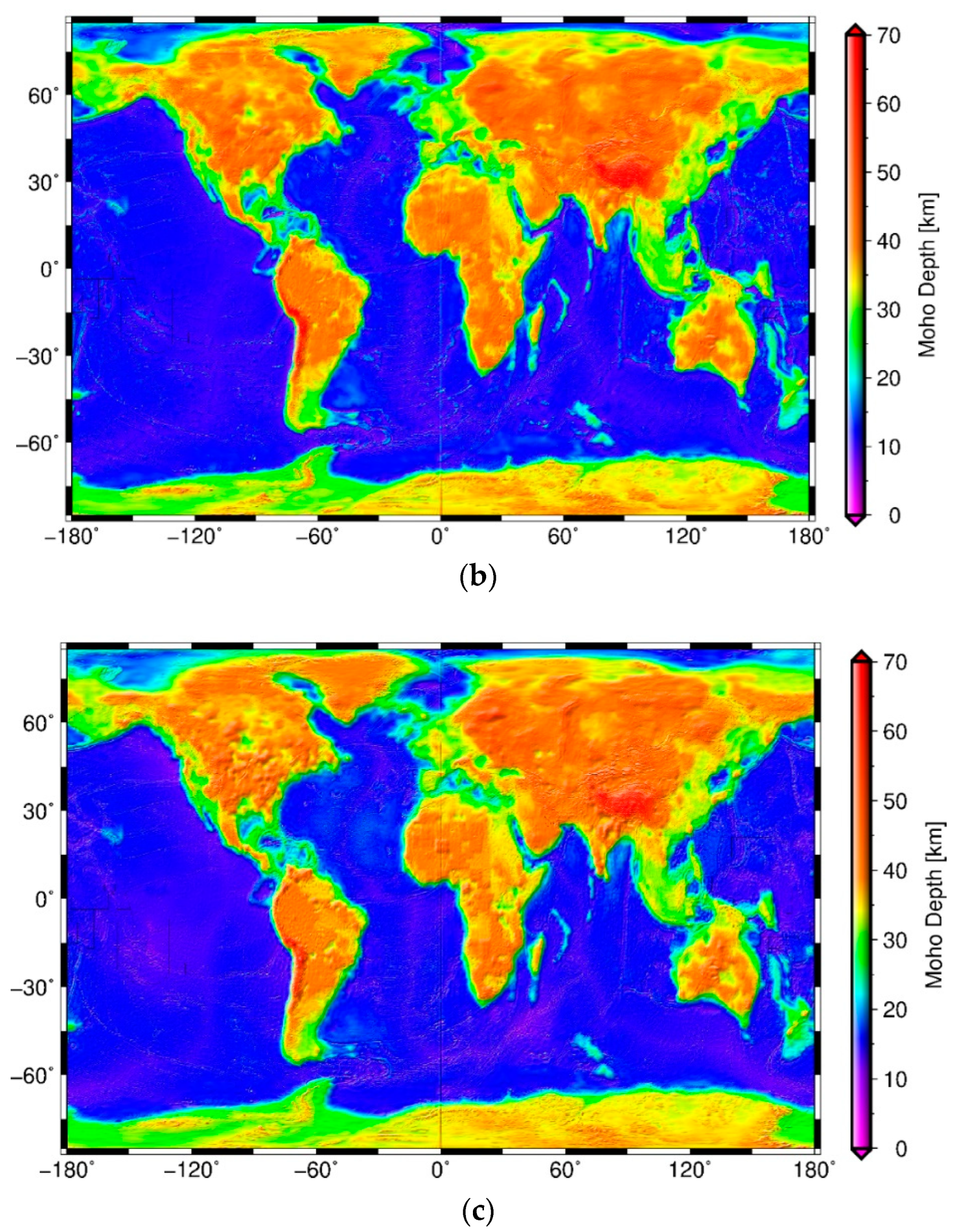
We applied the Butterworth filtering and spectral combination techniques to compile two global high-resolution combined Moho (HRCM) models on a 5’ × 5’ grid by integrating the CRUST1.0 seismic and VMM Moho depth models according to Equations (14) and (24). The parameters n b and k of the Butterworth filter were selected carefully. The value n b = 78 was obtained on the basis of the analysis of power–degree variances of the CRUST1.0 model, where n b defines the degree at which the power is halved (cut-off degree). In addition, we checked the sensitivity of HRCM results for different values of the k parameter. For this purpose, we used the continental and regional Moho depth models that were later used to validate our HRCMs. As seen in Table 1, different choice of the k-value does not significantly affect the RMS fit of the HRCMs with the continental/regional Moho models. Hence, we used only the result of the Butterworth filter for k = 1 in the spectral combination.
It is worth noting that despite the value n b = 78 being found to be optimal for combining the CRUST1.0 and VMM Moho depth models globally, it is very likely that such spectral resolution of the CRUST1.0 Moho model might not realistically reproduce the Moho geometry in many parts of the world that are characterized by a sparse or irregular seismic data coverage, particularly in Africa and South America. In regional studies, therefore, this parameter has to be selected specifically from gravity and seismic datasets available for a particular study area.
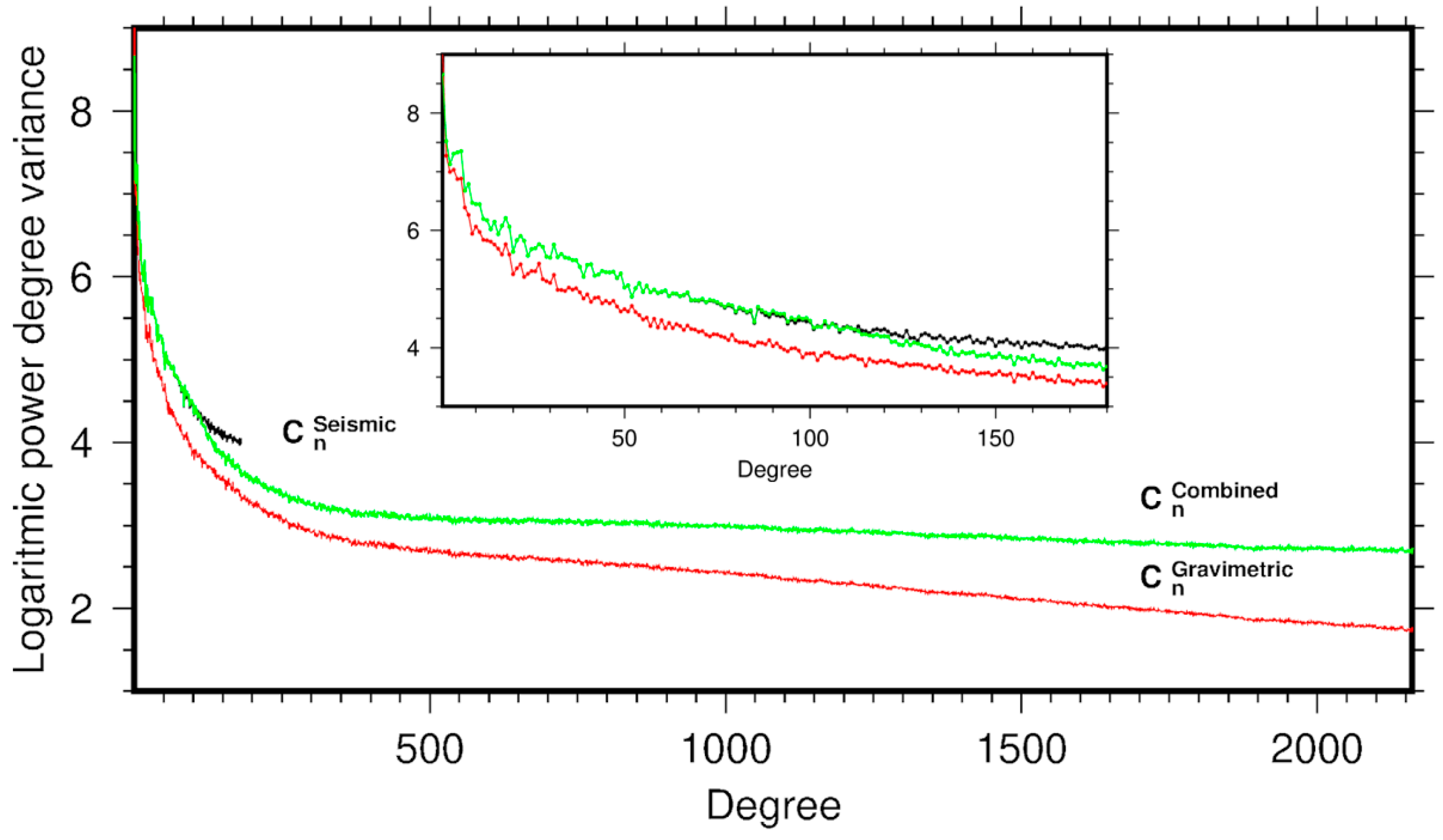
The HRCM model compiled by applying the Butterworth filter was obtained by fitting the linear regression to the logarithmic power–degree variances of the CRUST1.0 and VMM models (see Figure 1). The lines were fitted between degrees 25 and 180 (which is the maximum degree of the CRUST1.0 model) by using the least-squares analysis because the Butterworth filter assigns higher weights to lower degrees of the CRUST1.0 model [39]. By applying this principle, the results are expected to be reasonably close to the seismic model (reality in this case). It is important to mention that we did not consider degrees below 25 in the linear regression model because they provide unrealistic results. As seen in Figure 1 and Figure 2, the curves (power–degree variances of the CRUST1 and VMM models) are vertically sharp (large slope) for degrees less than 25, and fitting lines to the power–degrees provide large differences (bias) with respect to the reference Moho models. In addition, we rely more on the CRUST1 model (by considering higher weights) up to degree of 78 (i.e., at long to medium wavelengths). According to Figure 1, we see that a shift can be computed (between blue and green lines) by considering fitted regression lines to degrees 25 and 180, and the fitted lines are parallel.
We obtained the fitted line equations of log ( c n s e i s m i c ) = 5.63 0.0105 n and log ( c n G r a v i m e t r i c ) = 5.18 0.0111 n for the CRUST1.0 and VMM models, respectively, by using the least-squares analysis. After calculating Δ a = a s e i s m i c a V M M and Δ b = b s e i s m i c b V M M in Equation (10), the HRCM model was computed according to Equations (11) and (14). The logarithmic power–degree variances of the HRCM model obtained from Equation (15) are presented in Figure 2. As seen, after the degree of 78 the HRCM model smoothly deviates from the CRUST1.0 model, and the Butterworth filter assigns higher weights to the corrected VMM Moho depth model. In other words, it uses the corrected short wavelengths of the VMM model (up to 2160 degrees) to model the detailed Moho pattern in the HRCM result. The CRUST1.0 Moho depth and the HRCM result obtained by applying the Butterworth filter are shown in Figure 3a,b, respectively.
To model the HRCM by using the spectral combination method, the coefficients of A ^ n and B ^ n were determined according to Equations (22) and (23). This procedure required the a priori information about uncertainties of the CRUST1.0 and VMM models. Since the uncertainty of the CRUST1.0 model is not officially provided, we considered 10% uncertainties of the CRUST1.0 model to determine σ D n s e i s m i c [44]. We further determined σ D n V M M by using the standard error of the spherical harmonic coefficients obtained from the XGM2019e model. The HRCM result obtained according to Equation (24) is presented in Figure 3c.
The HRCM Moho depth obtained by applying the Butterworth filter varies between 75 and 3.5 km, with a mean of 26.5 km and a standard deviation of 12.5 km. The corresponding continental and oceanic mean Moho depths are 37.2 and 15.8 km, respectively. For the spectral combination method, the Moho depth variations are between 75.6 and 4.5 km, with a mean of 24.7 km and a standard deviation of 11.0 km. The corresponding continental and oceanic mean Moho depths are 37.3 and 18.7 km, respectively. The presented results in Figure 3b,c are satisfactory and close to the regional Moho depth models that we used for the validation (see Table 1 as well as Section 4.2). As aforestated, the newly developed HRCMs could be used, for instance, to study subduction zones, where the geometry and physical characteristics (such as a crust–mantle density contrast) of the Moho interface vary significantly, even on a local scale. It is also worth noting that both HRCMs solutions (Figure 3b,c) have been computed with a spatial resolution that is much higher than a spatial resolution of the CRUST1.0 (Figure 3a).
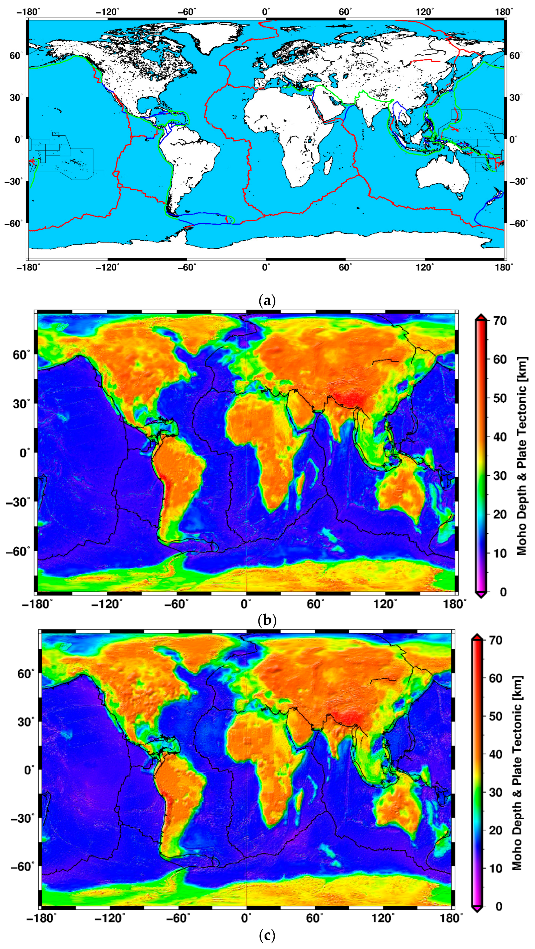
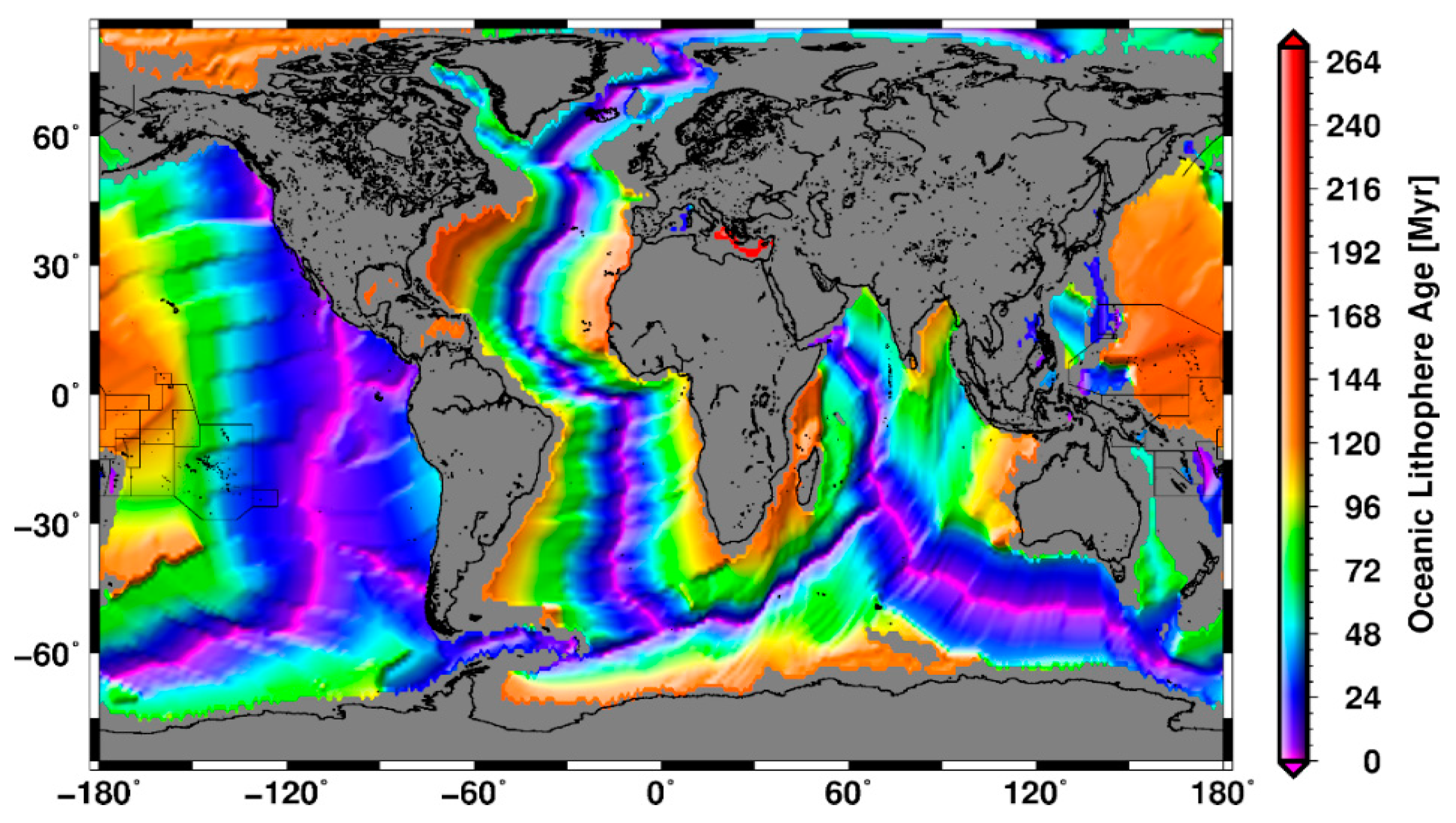
As expected, the HRCM solutions provide a thin crustal thickness along oceanic ridges characterized by a young oceanic lithosphere; see Figure 4. The oceanic lithosphere age dataset was provided by [45]. It is worth noting that the relationship between the ocean-floor spreading (i.e., the oceanic lithosphere age) and the Moho parameters (i.e., the Moho depth and density contrast) can be used to further analyze geodynamic processes associated with the oceanic lithospheric cycle [17]. Under the continental crust, the HRCM Moho depth maxima are seen along active convergent tectonic margins (Figure A4) that formed major orogenic belts of Himalaya and Tibet Plateau (with the maximum Moho depth of 77 km) and Andes (with the maximum Moho depth of 71 km).

4.2. Validation

We used the Moho models [5,29,30,31,32] to assess the accuracy of HRCM solutions obtained by applying the Butterworth filtering and spectral combination techniques. Table 2 summarizes statistics of the Moho depth differences between both results and validation models. The comparison shows that the RMS of Moho depth differences varies between 1.7 and 4.7 km when using the Butterworth filter and between 0.41 and 4.1 km when employing the spectral combination. We note that both HRCM solutions were resampled from a 5’ × 5’ to 1° × 1° grid in order to become compatible with the models of [5,29,30,31,32] used for the validation. It is important to note that there are some substantial differences in Europe between the Eurasian Moho model [5] and the European Plate Moho model [29]. These differences (shown in Figure A2) are due to applying different methods and partially due to some differences between seismic datasets used to compile these two models. We, therefore, used both models in our comparison.
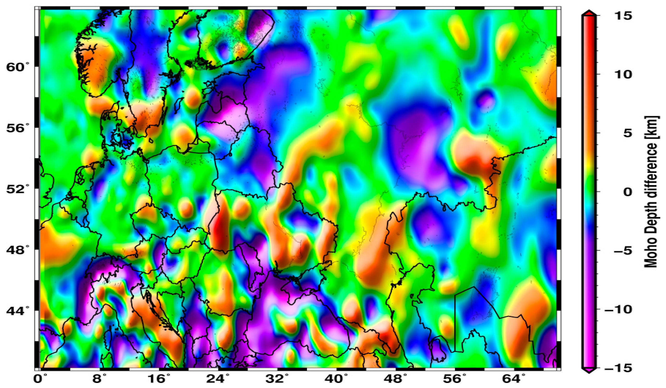
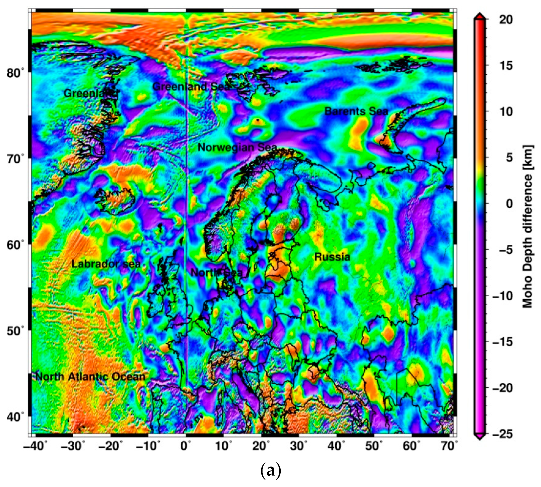
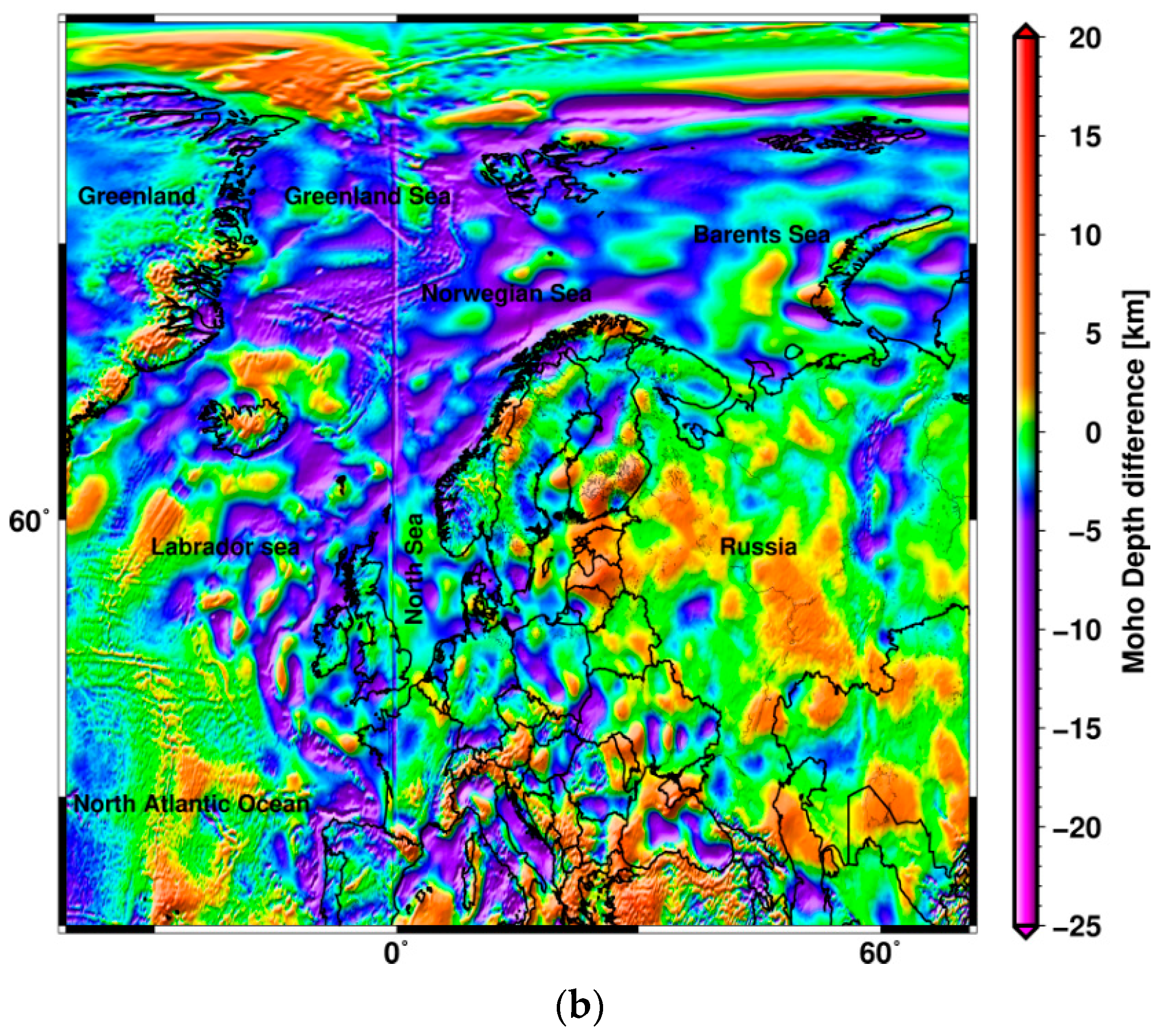
Figure 5 shows the Moho depth differences between the HRCMs and the Eurasian Moho model [5]. As already mentioned, this comparison was performed after resampling the HRCM models to a 1° × 1° grid. The RMS of the Moho depth differences is 2.9 and 2.4 km for the Butterworth filtering and spectral combination techniques, respectively (see Table 2). Most of these differences (86%) in Eurasia are within ±5 km (see Table 3). The best compliance was obtained in the European region. The same comparison was conducted by using the European Plate Moho model [29] in Figure 6. Despite a generally good agreement between the HRCMs and European Plate Moho models, some large Moho depth differences could also be recognized in areas without a regional seismic or gravity data coverage (usually along margins of the European Plate) that were filled by data from more general low-resolution global models [46,47]; for more information see [29].
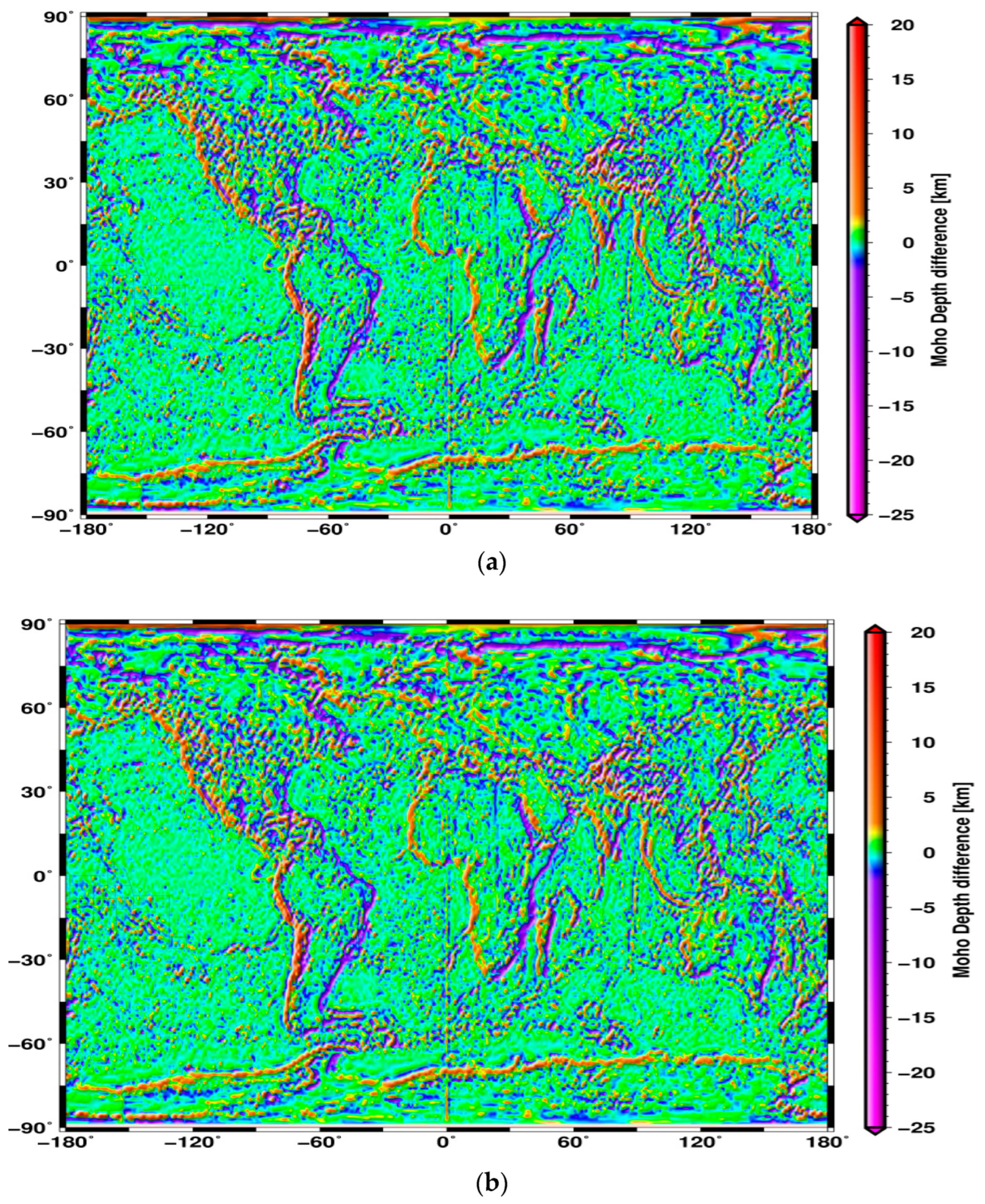
In Appendix A, we compared the Moho depth differences of both HRCM solutions with respect to the CRUST1.0 Moho depths (see Figure A3). Large differences, in this case, are seen along continental margins and oceanic ridges. There are some areas where large differences are likely due to unmodelled density variations within the lithospheric crust. Elsewhere, the Moho depth results are generally consistent. Part of these differences (in Table 2) could be due to the selection of the uncertainty value in the used data (assuming 10% uncertainty for the CRUST1.0) and models in our algorithm.
As seen in Figure 5 and Figure 6, large Moho depth differences between the HRCM solutions and the Eurasian and European Plate Moho models are detected along continental margins and in polar regions. These large differences might be explained by large sedimentary basins and rigidity variations of the crustal plate [48]. In addition, it is worth noting that the CRUST1.0 datasets, particularly sediment and consolidated (crystalline) crust datasets used to compute the Bouguer gravity data, often have a low accuracy and resolution.
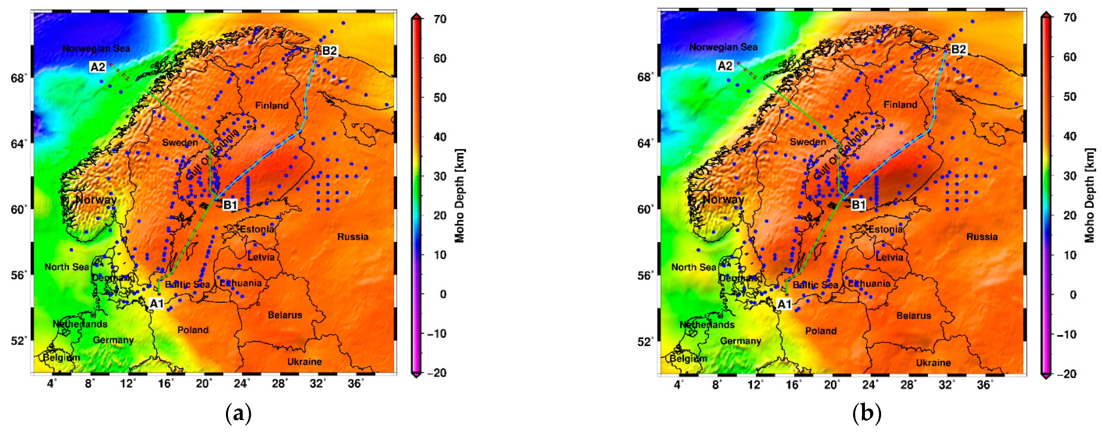
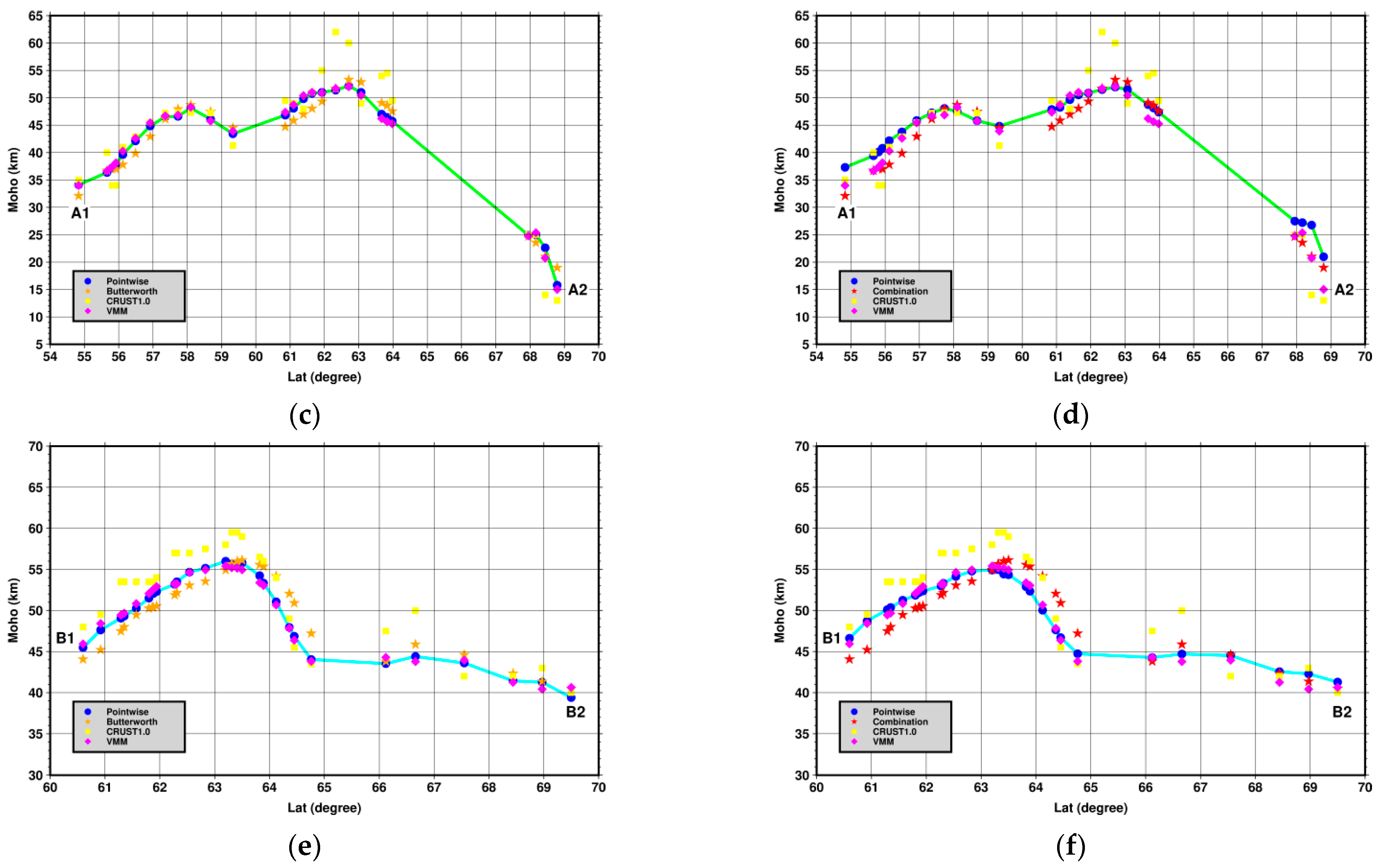
We further compared the HRCM solutions with the point-wise seismic Moho depth estimates at 308 stations in the Fennoscandia Shield [30]. Figure 7a,b depict the detailed Moho geometry in Fennoscandia according to our two HRCM models. For a more detailed analysis, we selected two profiles, A1–A2 and B1–B2 (see Figure 7a, b and Table 4), so that they cross the lowest and highest altitudes of the region as well the sea and the land. The HRCM solutions are compared with the point-wise data along both profiles in Figure 7c,d. Along the A1–A2 profile crossing the Baltic Sea, we see larger Moho depth differences between the HRCMs and the point-wise seismic data at the beginning of the profile. A better agreement of our results with seismic estimates is seen along the B1-B2 profile that intersects the largest Moho depths in Fennoscandia. The RMS of differences along the A1-A2 and B1-B2 profiles is 2.9 km (for the HRCM Butterworth filter solution) and 2.2 km (for the HRCM spectral combination solution).
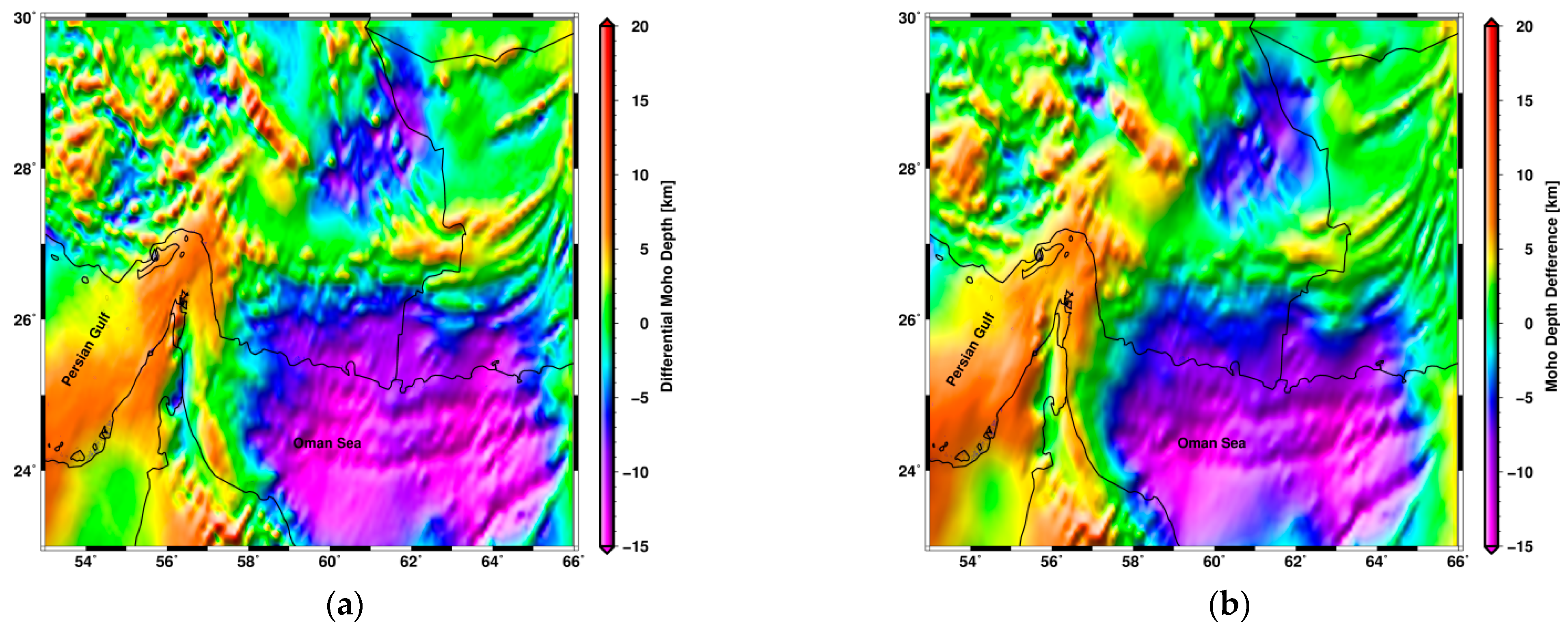
To inspect the performance of our two methods for a region characterized by a complex tectonic configuration, we compared the HRCM solutions with the Moho depth estimates in the Makran subduction zone [31]. The Moho depth differences are plotted in Figure 8. The RMS of Moho depth differences are 4.7 and 4.1 km for the HRCM solutions obtained by applying the Butterworth filter and spectral combination techniques, respectively (see Table 1). As seen, both HRCM solutions have been able to depict relatively closely the Moho geometry derived from the regional model [31] in the study area. One of our goals in developing HRCM models is to model the Moho in regions with specific tectonics. Makran is a subduction zone that is very unknown due to the low number of seismic mapping stations, and few studies have been conducted in this area. As a result, we attempted to show the HRCM model discrepancy with respect to other models in Makran. It is obvious that there are many subduction zones in the world, but Makran has a high tectonic complexity and suffers from a lack of proper study and data [49]. However, the obtained RMS values are acceptable compared with the state of the complexity of subduction in Makran. It is also worth mentioning that we used a recently published data set [31] in Makran for our comparison.
Finally, we validated the HRCM models by using the United States Moho model [32]. The Moho depth differences are plotted in Figure 9. The RMS of Moho depth differences are 1.0 and 2.1 km for the HRCM results obtained by applying the Butterworth filter and spectral combination techniques, respectively (see Table 1). The eastern Cascadia subduction zone, which also effects of subduction procedure in the U.S., is included in the dataset [32] for comparison in this paper.

5. Conclusions

The existing global seismic Moho depth models (e.g., CRTUST1.0) have a limited resolution as well as the accuracy in large parts of the world where the seismic data coverage is insufficient. Global gravitational models, on the other hand, provide the homogenous information about the gravity field globally and with a spatial resolution that allows estimation of the Moho depth with a high resolution. The gravimetric forward and inverse methods developed for a Moho modelling are, however, not unique due to large uncertainties of existing global crustal structure models as well as typically (unmodelled) mantle density heterogeneities that also affect results of a gravimetric Moho modelling, especially at medium and long wavelengths. Moreover, the gravimetric inversion procedure is ill-posed. The solution is non-unique unless additional constraints are applied or assumptions are adopted. Classical isostatic theories, such as Airy’s and Pratt’s hypotheses, do not require directly the gravity information. However, their application is restricted by many theoretical limitations, such as the consideration of a localized instead of regional compensation mechanism, the fact that the isostatic balance takes place at depths within the mantle lithosphere rather than within the crust only, and the existence of isostatically uncompensated lithospheric structures particularly along active convergent and divergent tectonic margins.
The most effective way to overcome practical limitations associated with a sparse and irregular seismic data coverage and theoretical deficiencies of gravimetric and isostatic models is based on an optimal combination of seismic and gravity data. As aforestated, global seismic models provide relatively realistic information about the global Moho geometry, while gravity data could be used as supplementary information to replicate a more detailed Moho pattern as well as to interpolate the Moho geometry where seismic data is sparse or missing.
In this study, we compared the performance of two methods for combining seismic and gravity data, particularly by applying the Butterworth filtering and spectral combination techniques. We applied both methods to combine the long-wavelength information about the Moho geometry from the CRUST1.0 global seismic model with the detailed gravity information about the Moho geometry obtained by solving the VMM inverse problem of isostasy. The results of this procedure were presented as the HRCM solutions and provided on a 5’ × 5’ global grid. Such high-resolution global Moho models are required in many disciplines in geology and geophysics for a better understanding of tectonic and geological processes. In addition, these models could provide more detailed information about upper mantle heterogeneities. Since the refined Bouguer gravity data used to estimate the VMM Moho depths were obtained by applying the topographic gravity correction together with additional gravity corrections due to crustal density heterogeneities (of ice, ocean, and sediments), we addressed a non-uniqueness of a gravimetric inversion by considering actual crustal density heterogeneities (up to the level of uncertainties of the CRUST1.0 crustal structure data). The combination of the gravimetric–isostatic result with seismic data further reduced additional errors in the long-wavelength Moho geometry attributed mainly to a deep mantle density structure controlled by a global mantle flow. In this way, the HRCMs have a much higher resolution than existing seismic and gravimetric Moho models, while also achieving the accuracy that is compatible with regional and continental Moho models.
The accuracy of the Butterworth and spectral combination techniques was assessed by using the continental and regional Moho depth models for Eurasia, Europe, Fennoscandia, the Makran subduction zone, and the United States prepared mostly from the seismic data. The validation of results revealed that the RMS of Moho depth differences is between 0.4 and 4.1 km for the HRCM spectral combination solution, while between 1.7 and 4.7 km for the HRCM Butterworth filter solution. This numerical finding indicates a better performance of the spectral combination technique. Nevertheless, the Butterworth technique provided a little better result in the United States and the Makran subduction zone. The comparison also indicates that both techniques provide results that more closely agree (by means of the RMS fit) with continental models, while larger discrepancies were found with respect to regional models used for the validation. This finding is not surprising because the parameters of the Butterworth filter and the spectral combination were set up to optimally combine the VMM and CRUST1.0 Moho depth models on a global scale.
The validation of the spectral combination technique demonstrated a good agreement of our result with Moho depth estimates over regions with sufficient coverage of high-quality seismic data, namely in parts of the United States and Europe. Much larger inconsistencies were, however, detected over regions with a low seismic data coverage.
The validation of our solutions at the Makran subduction zone confirmed the capability of the proposed techniques to model a Moho geometry quite realistically, even under the crust characterized by a complex tectonic setting. It is also possible to improve existing models locally by applying proposed techniques while using regional or local seismic data. The seismic data coverage obviously significantly affects uncertainties in estimated Moho depths. It is also worth noting that the CRUST1.0 density uncertainties propagate to errors in estimated Moho depths. Large errors were found, for instance, along continental margins of the Eurasian tectonic plate characterized by large sediment deposits that could likely be explained by uncertainties in the CRUST1.0 sediment data. Additional errors are attributed to large rigidity variations of the crustal plate that could not readily be modelled by the VMM isostatic model without using a sufficiently detailed seismic and density data.
Despite these deficiencies, the proposed techniques provided substantially improved results (at least from a resolution point of view) even in regions without sufficient seismic data coverage, specifically in parts of Afghanistan, Pakistan, Mongolia and Far East Russia, the Arabian Peninsula, and near the Afar triple junction in East Africa. Obviously, these results could further be improved by integrating multiple regional Moho depth models and employing them in the suggested techniques applied in this study. Finally, one of the issues that should be considered in future studies is the investigation of the influence of sedimentary basins on the Moho depth estimates by using a global sedimentary data [49].

Author Contributions

A.D., conceived and performed the experiments, analyzed and interpreted the data, developed the software package, and wrote the first draft of the paper; M.B., proposed, conceived, and designed the study, prepared input data, developed the software package, performed the experiments, and analyzed and interpreted the results; B.V., analyzed and interpreted the data; R.T., contributed to the design of the paper and interpreted the results. All authors have read and agreed to the published version of the manuscript.

Funding

This research received no external funding.

Data Availability Statement

The data that support the findings of this study are available from the corresponding author on request.

Acknowledgments

The unknown reviewers and editor are sincerely appreciated for their constructive comments that helped to improve the manuscript.

Conflicts of Interest

The authors declare no conflict of interest.

Appendix A

Figure A1. The differences between the VMM Moho depth estimates from the EGM2008 and EIGEN-6C4 gravitational models. Unit: km.
Remotesensing 15 01562 g0a1
Table A1. The Moho depth differences obtained by solving the VMM problem by using the EGM2008 and EIGEN-6C4 gravitational models. Unit: Percentage (%).
DifferencesPercentage (%)
Less than |±1| km100
Less than |±0.5| km 99
Less than |±0.2| km 92
Table A2. Statistics of the Moho depth differences obtained by solving the VMM problem by using the EGM2008 and EIGEN-6C4 gravitational models. Unit: km.
Statistical ParametersValue
Max−4.0
Mean−0.0
Min−3.5
STD0.1
Figure A2. The Moho depth differences between the Eurasian [5] and European [29] models within Europe. Unit: km.
Remotesensing 15 01562 g0a2
Figure A3. The Moho depth differences between (a) the HRCM Butterworth filter solution and the CRUST1.0 model [27] and (b) the HRCM spectral combination solution and the CRUST1.0 model [27]. Unit: km.
Remotesensing 15 01562 g0a3
Figure A4. The Moho geometry and global tectonic configuration: (a) The Earth’s tectonic margins (red = divergent plate boundary, green = convergence plate boundary, and blue = transform plate boundary), (b) the HRCM Butterworth filter solution including tectonic configuration, and (c) the HRCM spectral combination solution including tectonic configuration.
Remotesensing 15 01562 g0a4

References

  1. Martinec, Z. The minimum depth of compensation of topographic masses. Geophys. J. Int. 1994, 117, 545–554. [Google Scholar] [CrossRef] [Green Version]
  2. Mooney, W.D.; Laske, G.; Masters, T.G. CRUST 5.1: A global crustal model at 5 × 5. J. Geophys. Res. Solid Earth 1998, 103, 727–747. [Google Scholar] [CrossRef]
  3. Akinrinade, O.J.; Li, C.-F.; Afelumo, A.J. Geodynamic processes inferred from Moho and Curie depths in Central and Southern African Archean Cratons. Tectonophysics 2021, 815, 228993. [Google Scholar] [CrossRef]
  4. Yuan, X.; Sobolev, S.V.; Kind, R. Moho topography in the central Andes and its geodynamic implications. Earth Planet. Sci. Lett. 2002, 199, 389–402. [Google Scholar] [CrossRef]
  5. Stolk, W.; Kaban, M.; Beekman, F.; Tesauro, M.; Mooney, W.D.; Cloetingh, S. High resolution regional crustal models from irregularly distributed data: Application to Asia and adjacent areas. Tectonophysics 2013, 602, 55–68. [Google Scholar] [CrossRef]
  6. Becker, T.W.; Faccenna, C. Mantle conveyor beneath the Tethyan collisional belt. Earth Planet. Sci. Lett. 2011, 310, 453–461. [Google Scholar] [CrossRef]
  7. Richards, M.A.; Hager, B.H. Geoid anomalies in a dynamic Earth. J. Geophys. Res. Solid Earth 1984, 89, 5987–6002. [Google Scholar] [CrossRef] [Green Version]
  8. Sjöberg, L.E.; Bagherbandi, M. Gravity Inversion and Integration; Springer: Berlin/Heidelberg, Germany, 2017. [Google Scholar]
  9. Ghomsi, F.E.K.; Tenzer, R.; Njinju, E.; Steffen, R. The crustal configuration of the West and Central African Rift System from gravity and seismic data analysis. Geophys. J. Int. 2022, 230, 995–1012. [Google Scholar] [CrossRef]
  10. Shin, Y.H.; Shum, C.; Braitenberg, C.; Lee, S.M.; Na, S.-H.; Choi, K.S.; Hsu, H.; Park, Y.-S.; Lim, M. Moho topography, ranges and folds of Tibet by analysis of global gravity models and GOCE data. Sci. Rep. 2015, 5, 11681. [Google Scholar] [CrossRef] [PubMed] [Green Version]
  11. Pratt, J.H.I. On the attraction of the Himalaya Mountains, and of the elevated regions beyond them, upon the plumb-line in India. Philos. Trans. R. Soc. Lond. 1855, 145, 53–100. [Google Scholar]
  12. Airy, G.B., III. On the computation of the effect of the attraction of mountain-masses, as disturbing the apparent astronomical latitude of stations in geodetic surveys. Philos. Trans. R. Soc. Lond. 1855, 145, 101–104. [Google Scholar] [CrossRef] [Green Version]
  13. Meinesz, F. Une nouvelle methode pour la reduction isostatique regionale de l’intensite de la pesanteur. Bull. Geod. 1931, 29, 33–51. [Google Scholar] [CrossRef]
  14. Moritz, H. The Figure of the Earth: Theoretical Geodesy and the Earth’s Interior; Wichmann: Karlsruhe, Germany, 1990. [Google Scholar]
  15. Sjöberg, L.E. Solving Vening Meinesz-Moritz inverse problem in isostasy. Geophys. J. Int. 2009, 179, 1527–1536. [Google Scholar] [CrossRef] [Green Version]
  16. Bagherbandi, M.; Eshagh, M. Combined Moho Estimators. Geodyn. Res. Int. Bull. 2014, 1, 1–11. [Google Scholar]
  17. Tenzer, R.; Chen, W. Expressions for the global gravimetric Moho modeling in spectral domain. Pure Appl. Geophys. 2014, 171, 1877–1896. [Google Scholar] [CrossRef]
  18. Wan, J.; Xu, C.; Luo, Z.; Wu, Y.; Zhou, B.; Yan, J. An Approach to Moho Topography Recovery Using the On-Orbit GOCE Gravity Gradients and Its Applications in Tibet. Remote Sens. 2019, 11, 1567. [Google Scholar] [CrossRef] [Green Version]
  19. Ye, Z.; Tenzer, R.; Sneeuw, N.; Liu, L.; Wild-Pfeiffer, F. Generalized model for a Moho inversion from gravity and vertical gravity-gradient data. Geophys. J. Int. 2016, 207, 111–128. [Google Scholar] [CrossRef]
  20. Bagherbandi, M.; Sjöberg, L.E. A synthetic Earth gravity model based on a topographic-isostatic model. Stud. Geophys. Geod. 2012, 56, 935–955. [Google Scholar] [CrossRef]
  21. Sjöberg, L.E.; Bagherbandi, M. A method of estimating the Moho density contrast with a tentative application of EGM08 and CRUST2.0. Acta Geophys. 2011, 59, 502–525. [Google Scholar] [CrossRef]
  22. Eshagh, M.; Bagherbandi, M.; Sjöberg, L. A combined global Moho model based on seismic and gravimetric data. Acta Geod. Geophys. Hung. 2011, 46, 25–38. [Google Scholar] [CrossRef]
  23. Reguzzoni, M.; Sampietro, D.; Sansò, F. Global Moho from the combination of the CRUST2.0 model and GOCE data. Geophys. J. Int. 2013, 195, 222–237. [Google Scholar] [CrossRef] [Green Version]
  24. Oppenheim, A.V.; Willsky, A.; Young, I. Signals and Systems; Prentice-Hall: Englewood Cliffs, NJ, USA, 2000. [Google Scholar]
  25. Sjöberg, L.E. Geoid determination by spectral combination of an Earth gravitational model with airborne and terrestrial gravimetry—A theoretical study. Stud. Geophys. Geod. 2011, 55, 579–588. [Google Scholar] [CrossRef]
  26. Bagherbandi, M. Combination of seismic and an isostatic crustal thickness models using Butterworth filter in a spectral approach. J. Asian Earth Sci. 2012, 59, 240–248. [Google Scholar] [CrossRef]
  27. Laske, G.; Masters, G.; Ma, Z.; Pasyanos, M. Update on CRUST1. 0—A 1-degree global model of Earth’s crust. In Proceedings of the Geophysical Research Abstracts, EGU General Assembly, Vienna, Austria, 7–12 April 2013. [Google Scholar]
  28. Bassin, C. The current limits of resolution for surface wave tomography in North America. Eos Trans. AGU 2000, 81, F897. [Google Scholar]
  29. Grad, M.; Tiira, T.; Group, E.W. The Moho depth map of the European Plate. Geophys. J. Int. 2009, 176, 279–292. [Google Scholar] [CrossRef] [Green Version]
  30. Luosto, U. Structure of the Earth’s crust in Fennoscandia as revealed from refraction and wide-angle reflection studies. Geophysica 1997, 33, 3–16. [Google Scholar]
  31. Abdollahi, S.; Ardestani, V.E.; Zeyen, H.; Shomali, Z.H. Crustal and upper mantle structures of Makran subduction zone, SE Iran by combined surface wave velocity analysis and gravity modeling. Tectonophysics 2018, 747, 191–210. [Google Scholar] [CrossRef]
  32. Zhang, H.; Ravat, D.; Lowry, A.R. Crustal composition and Moho variations of the central and eastern United States: Improving resolution and geologic interpretation of EarthScope USArray seismic images using gravity. J. Geophys. Res. Solid Earth 2020, 125, e2019JB018537. [Google Scholar] [CrossRef]
  33. Silvennoinen, H.; Kozlovskaya, E.; Kissling, E.; Kosarev, G.; W.L.P Group. A new Moho boundary map for the northern Fennoscandian Shield based on combined controlled-source seismic and receiver function data. GeoResJ 2014, 1, 19–32. [Google Scholar] [CrossRef] [Green Version]
  34. Lowry, A.R.; Pérez-Gussinyé, M. The role of crustal quartz in controlling Cordilleran deformation. Nature 2011, 471, 353–357. [Google Scholar] [CrossRef]
  35. Zingerle, P.; Pail, R.; Gruber, T.; Oikonomidou, X. The combined global gravity field model XGM2019e. J. Geod. 2020, 94, 66. [Google Scholar] [CrossRef]
  36. Shako, R.; Förste, C.; Abrikosov, O.; Bruinsma, S.; Marty, J.-C.; Lemoine, J.-M.; Flechtner, F.; Neumayer, H.; Dahle, C. EIGEN-6C: A high-resolution global gravity combination model including GOCE data. In Observation of the System Earth from Space-CHAMP, GRACE, GOCE and Future Missions; Springer: Berlin/Heidelberg, Germany, 2014; pp. 155–161. [Google Scholar]
  37. Pavlis, N.K.; Holmes, S.A.; Kenyon, S.C.; Factor, J.K. The development and evaluation of the Earth Gravitational Model 2008 (EGM2008). J. Geophys. Res. Solid Earth 2012, 117, B4. [Google Scholar] [CrossRef] [Green Version]
  38. Hirt, C.; Rexer, M. Earth2014: 1 arc-min shape, topography, bedrock and ice-sheet models–Available as gridded data and degree-10,800 spherical harmonics. Int. J. Appl. Earth Obs. Geoinf. 2015, 39, 103–112. [Google Scholar] [CrossRef] [Green Version]
  39. Haagmans, R. A synthetic Earth for use in geodesy. J. Geod. 2000, 74, 503–511. [Google Scholar] [CrossRef]
  40. Bagherbandi, M.; Sjöberg, L.E. Non-isostatic effects on crustal thickness: A study using CRUST2.0 in Fennoscandia. Phys. Earth Planet. Inter. 2012, 200, 37–44. [Google Scholar] [CrossRef]
  41. Claessens, S. A Synthetic Earth Model Analysis, Implementation, Validation and Application. Master’s Thesis, Delft University of Technology, Delft, The Netherlands, 2002. [Google Scholar]
  42. Kuhn, M.; Featherstone, W. On the construction of a synthetic Earth gravity model. In Proceedings of the Proceed 3rd Meeting of the International Gravity and Geoid Commission, Hrsg. I. Tziavos, Thessaloniki, Greece, 26–30 August 2002; pp. 189–194. [Google Scholar]
  43. Heiskanen, W.A. Physical geodesy. Determ. Geoid Ground Anom. 1967, 8, 325–330. [Google Scholar] [CrossRef]
  44. Čadek, O.; Martinec, Z. Spherical harmonic expansion of the Earth’s crustal thickness up to degree and order 30. Stud. Geophys. Geod. 1991, 35, 151–165. [Google Scholar] [CrossRef]
  45. Müller, R.D.; Sdrolias, M.; Gaina, C.; Roest, W.R. Age, spreading rates, and spreading asymmetry of the world’s ocean crust. Geochem. Geophys. Geosystems 2008, 9. [Google Scholar] [CrossRef]
  46. Laske, G. Crustal Model at 2 × 2 arc-degrees. 2002. Available online: http://igppweb.ucsd.edu/~gabi/rem.html (accessed on 27 November 2022).
  47. Pasyanos, M.E.; Walter, W.R.; Flanagan, M.P.; Goldstein, P.; Bhattacharyya, J. Building and testing an a priori geophysical model for western Eurasia and North Africa. Pure Appl. Geophys. 2004, 161, 235–281. [Google Scholar] [CrossRef]
  48. Braitenberg, C.; Wienecke, S.; Wang, Y. Basement structures from satellite-derived gravity field: South China Sea ridge. J. Geophys. Res. Solid Earth 2006, 111, B5. [Google Scholar] [CrossRef]
  49. Evenick, J.C. Glimpses into Earth’s history using a revised global sedimentary basin map. Earth-Sci. Rev. 2021, 215, 103564. [Google Scholar] [CrossRef]
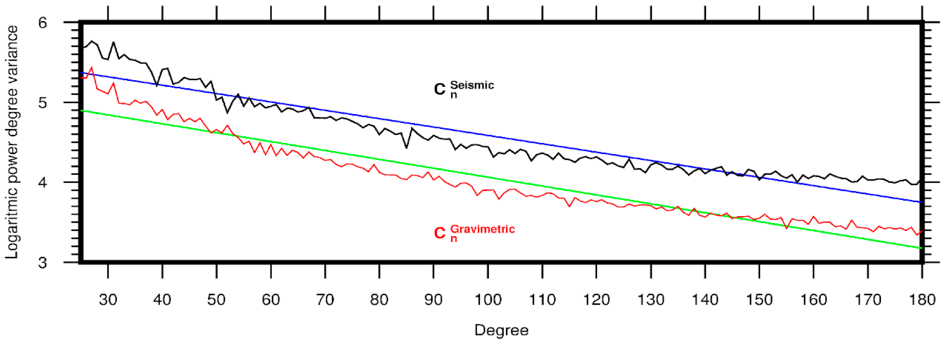
Figure 1. The logarithmic power–degree variances of the CRUST1.0 (black line), VMM (red line), and fitted regression lines between degrees 25 and 180. Blue and green lines are the fitted lines to the CRUST1 and VMM models, respectively. “Seismic” and “gravimetric” denote the CRUST1.0 and VMM models, respectively.
Remotesensing 15 01562 g001
Figure 2. The logarithmic power–degree variances of the CRUST1.0 model (black), the VMM model (red), and the HRCM solution (green) obtained by applying the Butterworth filter.
Remotesensing 15 01562 g002
Figure 3. Global Moho depth models: (a) the CRUST1.0 model (with the resolution of 1° × 1°), (b) the HRCM model obtained by applying the Butterworth filter (with the resolution of 5’ × 5’), and (c) the HRCM model obtained by using the spectral combination method (with the resolution of 5’ × 5’).
Remotesensing 15 01562 g003aRemotesensing 15 01562 g003b
Figure 4. The age of the oceanic lithosphere according to [45].
Remotesensing 15 01562 g004
Figure 5. The Moho depth differences between (a) the HRCM Butterworth filter solution and the Eurasian Moho model [5] and (b) the HRCM spectral combination solution and the Eurasian Moho model [5]. Unit: km.
Remotesensing 15 01562 g005aRemotesensing 15 01562 g005b
Figure 6. The Moho depth differences between (a) the HRCM Butterworth filter solution and the European Plate Moho model [29] and (b) the HRCM spectral combination solution and the European Plate Moho model [29]. Unit: km.
Remotesensing 15 01562 g006aRemotesensing 15 01562 g006b
Figure 7. The HRCM Moho depth solutions obtained by applying: (a) the Butterworth filter and (b) the spectral combination. Seismic profiles A1–A2 and B1–B2 are indicated by green and blue lines, respectively. Locations of seismic stations are indicated by blue dots. The Moho depth differences between the HRCM Butterworth filter solution and the point-wise seismic Fennoscandia Moho depth estimates [30] along (c) the A1–A2 and (e) B1–B2 profiles. The Moho depth differences between the HRCM spectral combination solution and the point-wise seismic Fennoscandia Moho depth estimates [30] along (d) the A1–A2 and (f) B1–B2 profiles. The HRCM Moho depth results are given on a 5’ × 5’ grid. Unit: km.
Remotesensing 15 01562 g007aRemotesensing 15 01562 g007b
Figure 8. The Moho depth differences between (a) the HRCM Butterworth filter solution and the Makran Moho model [31] and (b) the HRCM spectral combination solution and the Makran Moho model [31]. Unit: km.
Remotesensing 15 01562 g008
Figure 9. The Moho depth differences between (a) the HRCM Butterworth filter solution and the United States Moho model [32] and (b) the HRCM spectral combination solution and the United States Moho model [32]. Unit: km.
Remotesensing 15 01562 g009
Table 1. RMS of the Moho depth differences between the results obtained by applying the Butterworth and spectral combination techniques and the continental and regional Moho depth models for Eurasia [5], Europe [29], Fennoscandia [30], Makran [31], and the U.S. [32]. Unit: km.
Method n b kEurasiaEuropeFennoscandiaMakranU.S.
Butterworth7812.91.73.94.81.9
22.91.74.14.81.9
82.91.74.34.81.9
252.91.74.54.72.0
Spectral combination12.40.44.04.52.1
Table 2. Statistics of the Moho depth differences between the HRCM solutions and the continental and regional Moho depth models [5,29,30,31,32]. Unit: km.
MethodStatistics EurasiaEuropeFennoscandiaMakran U.S.
ButterworthMax37.820.78.619.539.8
Mean0.81.1−1.2−2.4−1.1
Min−23.1−27.6−15.6−46.6−13.4
RMS2.91.72.84.71.9
Spectral
Combination
Max38.115.612.814.239.5
Mean−0.7−1.1−0.1−1.01−2.0
Min−20.8−19.1−14.1−46.6−13.0
RMS2.40.42.94.12.1
Table 3. Statistics of the HRCM Moho depth differences with respect to the continental and regional Moho models [5,29,30,31,32].
MethodDifferencesEurasia
(%)
Europe
(%)
Fennoscandia
(%)
Makran
(%)
U.S.
(%)
ButterworthLess than ±5 km86 90 100 6198
Less than ±10 km9799 100 85 100
Spectral
Combination
Less than ±5 km8692956286
Less than ±10 km98 100 100 9199
Table 4. Statistics of the HRCM Moho depth differences with respect to the point-wise seismic Fennoscandia Moho depth estimates [30] along the A1-A2 and B1-B2 profiles. Unit: km.
Profiles
HRCM Models A1–A2B1–B2
ButterworthMax8.61.6
Mean−1.1−2.3
Min−10.6−5.6
RMS2.92.0
Spectral
Combination
Max12.82.6
Mean0.4−2.2
Min−10.5−5.3
RMS3.42.1
Disclaimer/Publisher’s Note: The statements, opinions and data contained in all publications are solely those of the individual author(s) and contributor(s) and not of MDPI and/or the editor(s). MDPI and/or the editor(s) disclaim responsibility for any injury to people or property resulting from any ideas, methods, instructions or products referred to in the content.