

An Efficient Channel Imbalance Estimation Method Based on Subadditivity of Linear Normed Space of Sub-Band Spectrum for Azimuth Multichannel SAR
 ,
,  , ,
, , 
Abstract
1. Introduction
2. Material
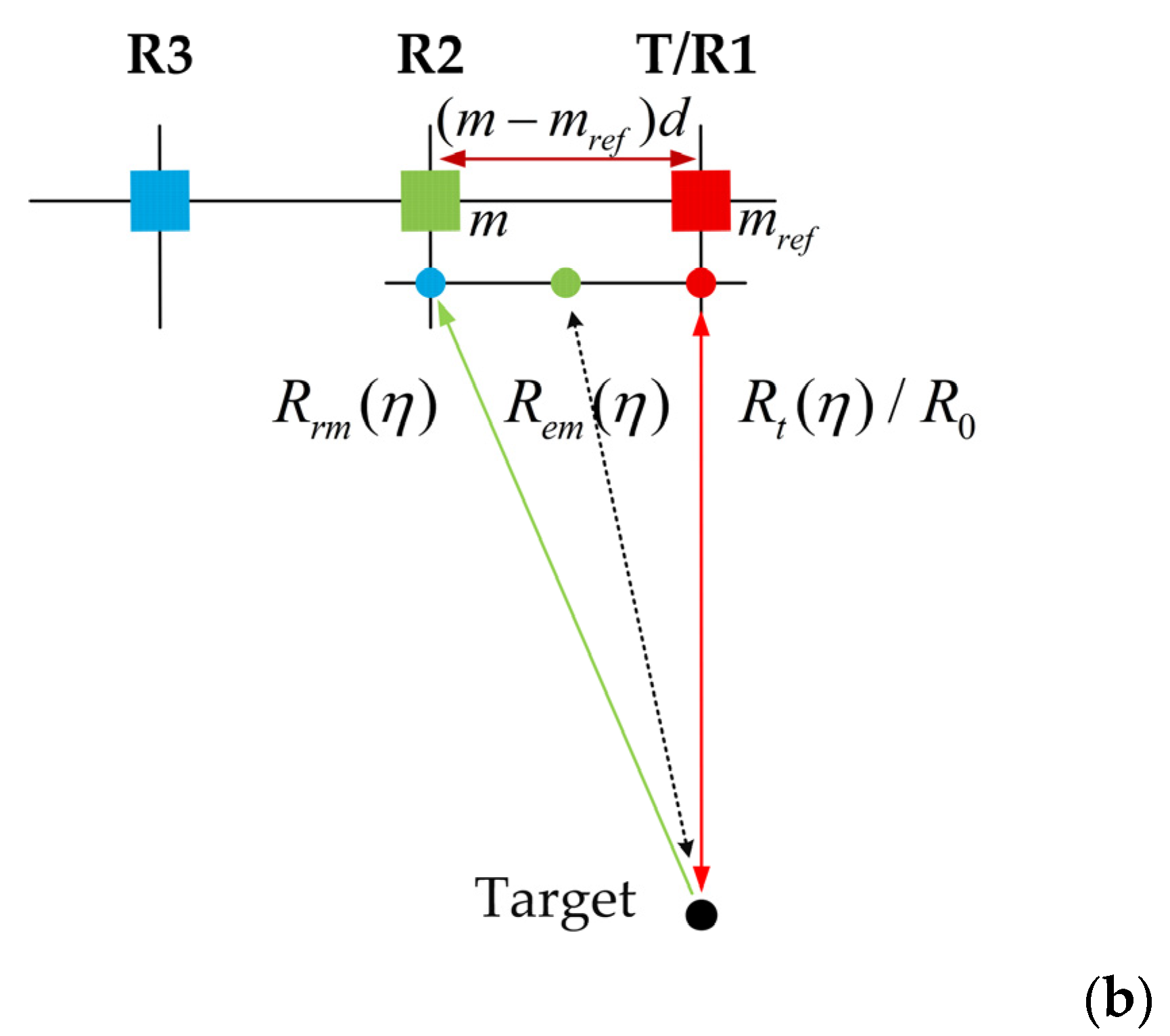
2.1. Signal Model
2.2. Signal Reconstruction
2.3. Channel Imbalance Analysis
2.3.1. Influence of Amplitude Imbalance
2.3.2. Influence of Phase Imbalance
2.3.3. Influence of RSTI
2.3.4. Influence of Antenna Position Imbalance
2.4. Precalibration Processing
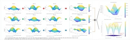
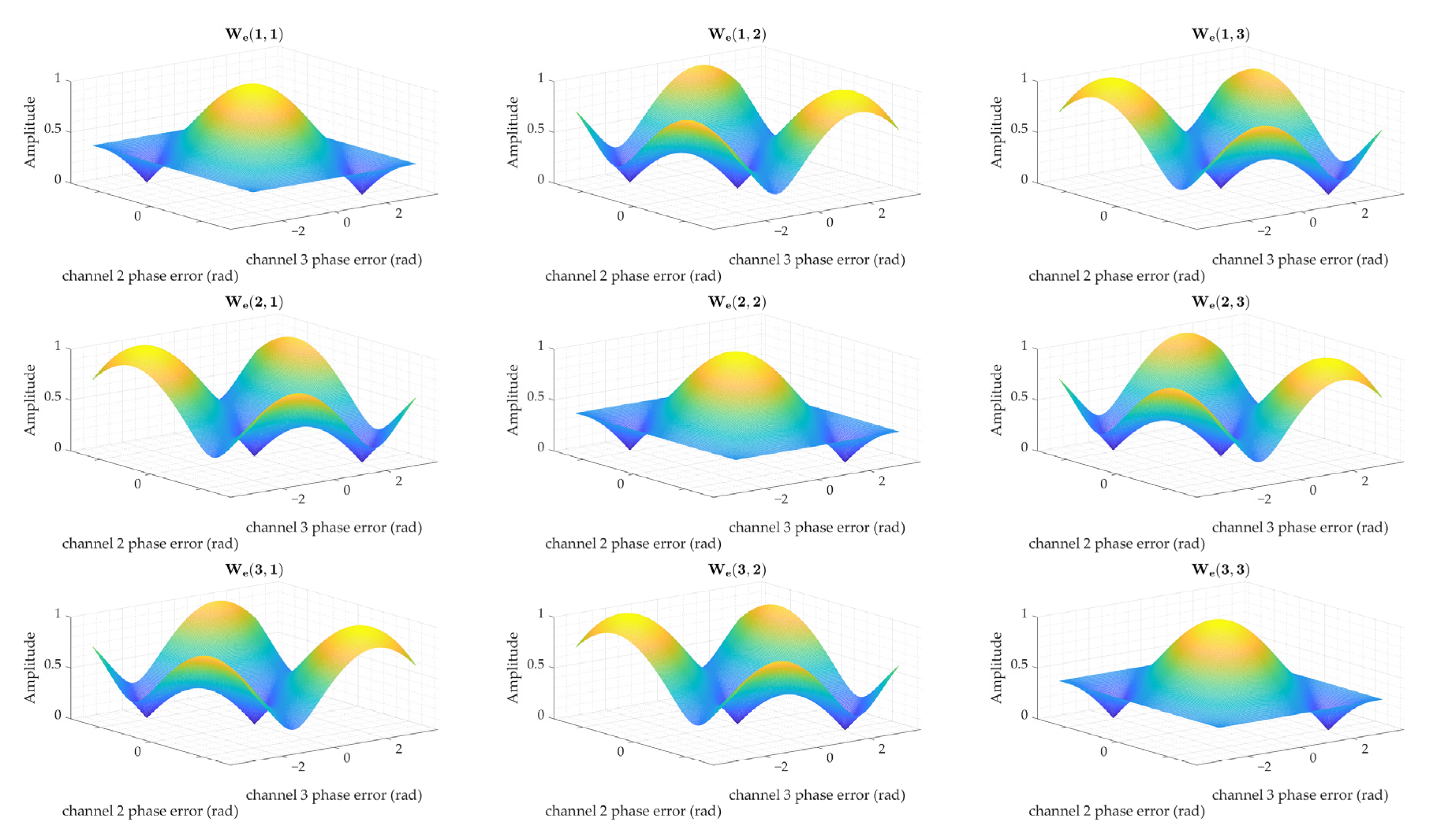
3. Method
4. Results and Discussions
4.1. Simulation Experiment and Results
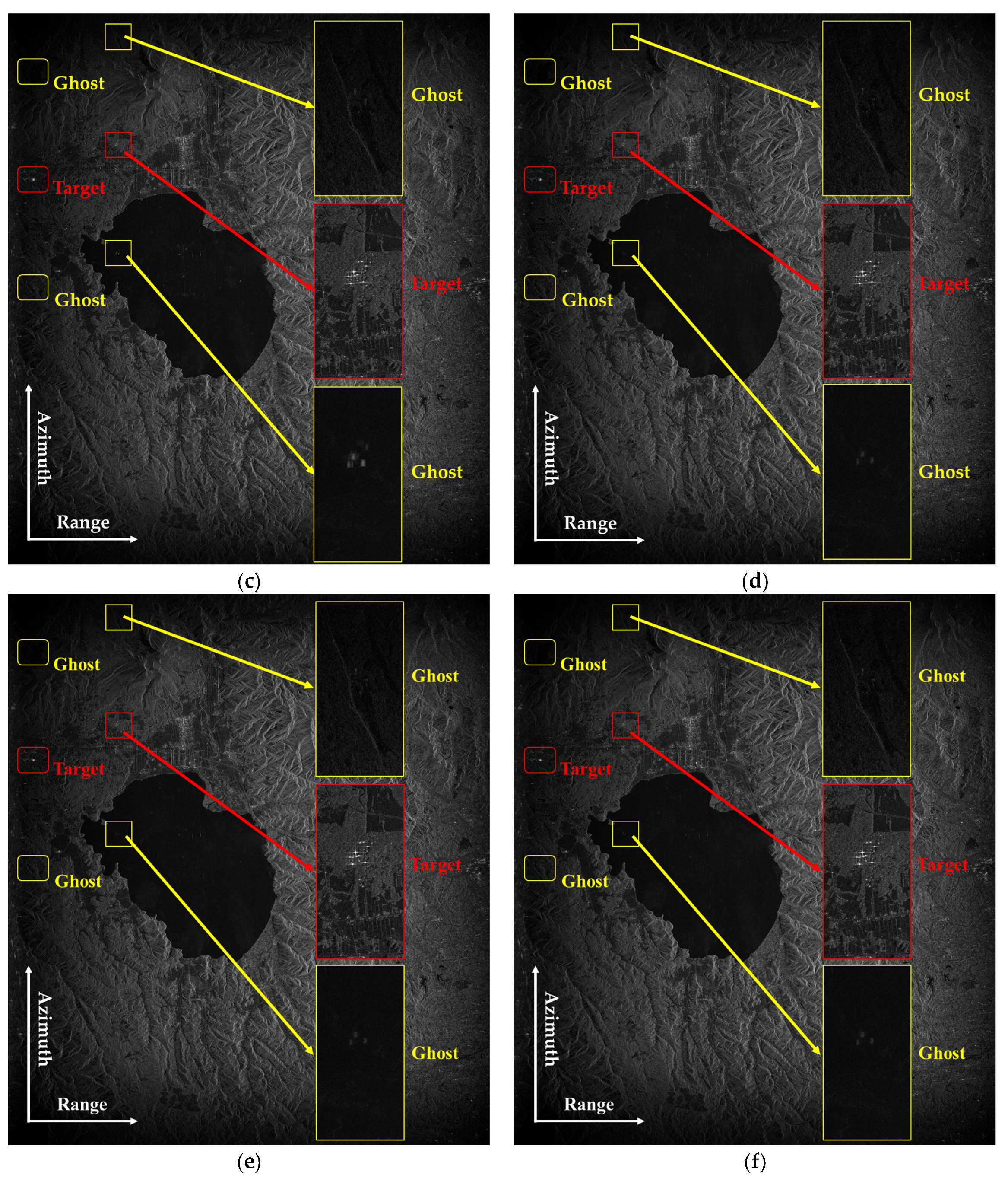
4.2. Experimental Results of GF-3 Measured Data
5. Conclusions
Author Contributions
Funding
Data Availability Statement
Conflicts of Interest
Appendix A
References
- Cumming, I.G.; Wong, F.H. Digital Processing of Synthetic Aperture Radar Data: Algorithms and Implementation; Artech House: Boston, MA, USA, 2005; Volume 1, pp. 108–110. [Google Scholar]
- Li, Z.; Wang, H.; Su, T.; Bao, Z. Generation of Wide-Swath and High-Resolution SAR Images From Multichannel Small Spaceborne SAR Systems. IEEE Geosci. Remote Sens. Lett. 2005, 2, 82–86. [Google Scholar] [CrossRef]
- Krieger, G.; Gebert, N.; Moreira, A. Unambiguous SAR Signal Reconstruction From Nonuniform Displaced Phase Center Sampling. IEEE Geosci. Remote Sens. Lett. 2004, 1, 260–264. [Google Scholar] [CrossRef]
- Krieger, G.; Gebert, N.; Moreira, A. Multidimensional waveform encoding: A new digital beamforming technique for synthetic aperture radar remote sensing. IEEE Trans. Geosci. Remote Sens. 2007, 46, 31–46. [Google Scholar] [CrossRef]
- Jing, W.; Xing, M.; Qiu, C.-W.; Bao, Z.; Yeo, T.-S. Unambiguous reconstruction and high-resolution imaging for multiple-channel SAR and airborne experiment results. IEEE Geosci. Remote Sens. Lett. 2008, 6, 102–106. [Google Scholar] [CrossRef]
- Krieger, G.; Gebert, N.; Younis, M.; Bordoni, F.; Patyuchenko, A.; Moreira, A. Advanced concepts for ultra-wide-swath SAR imaging. In Proceedings of the 7th European Conference on Synthetic Aperture Radar, Friedrichshafen, Germany, 2–5 June 2008; pp. 1–4. [Google Scholar]
- Yunkai, D.; Weidong, Y.; Heng, Z.; Wei, W.; Dacheng, L.; Robert, W. Forthcoming spaceborne SAR development. J. Radars 2020, 9, 1–33. [Google Scholar]
- Fu, Z.; Zhang, H.; Zhao, J.; Li, N.; Zheng, F. A Modified 2-D Notch Filter Based on Image Segmentation for RFI Mitigation in Synthetic Aperture Radar. Remote Sens. 2023, 15, 846. [Google Scholar] [CrossRef]
- Currie, A.; Brown, M.A. Wide-swath SAR. IEE Proc. F 1992, 139, 122–135. [Google Scholar] [CrossRef]
- Callaghan, G.; Longstaff, I. Wide-swath space-borne SAR using a quad-element array. IEE Proc.-Radar Sonar Navig. 1999, 146, 159–165. [Google Scholar] [CrossRef]
- Ender, J.H.; Klare, J. System architectures and algorithms for radar imaging by MIMO-SAR. In Proceedings of the 2009 IEEE Radar Conference, Pasadena, CA, USA, 4–8 May 2009; pp. 1–6. [Google Scholar]
- Süß, M.; Grafmüller, B.; Zahn, R. A novel high resolution, wide swath SAR system. In Proceedings of the IGARSS 2001. Scanning the Present and Resolving the Future. In Proceedings of the IEEE 2001 International Geoscience and Remote Sensing Symposium (Cat. No. 01CH37217), Sydney, Australia, 9–13 July 2001; pp. 1013–1015. [Google Scholar]
- Moore, R.K.; Claassen, J.P.; Lin, Y. Scanning spaceborne synthetic aperture radar with integrated radiometer. IEEE Trans. Aerosp. Electron. Syst. 1981, AES-17, 410–421. [Google Scholar] [CrossRef]
- Soumekh, M. Synthetic Aperture Radar Signal Processing; Wiley: New York, NY, USA, 1999; Volume 7. [Google Scholar]
- De Zan, F.; Guarnieri, A.M. TOPSAR: Terrain observation by progressive scans. IEEE Trans. Geosci. Remote Sens. 2006, 44, 2352–2360. [Google Scholar] [CrossRef]
- Naftaly, U.; Levy-Nathansohn, R. Overview of the TECSAR satellite hardware and mosaic mode. IEEE Geosci. Remote Sens. Lett. 2008, 5, 423–426. [Google Scholar] [CrossRef]
- Younis, M.; Fischer, C.; Wiesbeck, W. Digital beamforming in SAR systems. IEEE Trans. Geosci. Remote Sens. 2003, 41, 1735–1739. [Google Scholar] [CrossRef]
- Yingjie, W.; Robert, W.; Weidong, Y.; Qingchao, Z.; Kaiyu, L.; Dacheng, L.; Yunkai, D.; Naiming, O.; Xiaoxue, J.; Heng, Z.; et al. See-Earth: SAR Constellation with Dense Time-SEries for Multi-dimensional Environmental Monitoring of the Earth. J. Radars 2021, 10, 842–864. [Google Scholar]
- Kim, J.-H.; Younis, M.; Prats-Iraola, P.; Gabele, M.; Krieger, G. First spaceborne demonstration of digital beamforming for azimuth ambiguity suppression. IEEE Trans. Geosci. Remote Sens. 2012, 51, 579–590. [Google Scholar] [CrossRef]
- Luscombe, A. Image quality and calibration of RADARSAT-2. In Proceedings of the 2009 IEEE International Geoscience and Remote Sensing Symposium, Cape Town, South Africa, 12–17 July 2009; pp. II757–II760. [Google Scholar]
- Shimada, M. ALOS-2 science program. In Proceedings of the 2013 IEEE International Geoscience and Remote Sensing Symposium-IGARSS, Melbourne, Australia, 21–26 July 2013; pp. 2400–2403. [Google Scholar]
- Qingjun, Z. System design and key technologies of the GF-3 satellite. Acta Geod. Et Cartogr. Sin. 2017, 46, 269. [Google Scholar]
- Sun, J.; Yu, W.; Deng, Y. The SAR payload design and performance for the GF-3 mission. Sensors 2017, 17, 2419. [Google Scholar] [CrossRef]
- Lin, H.; Deng, Y.; Zhang, H.; Liu, D.; Liang, D.; Fang, T.; Wang, R. On the Processing of Dual-Channel Receiving Signals of the LuTan-1 SAR System. Remote Sens. 2022, 14, 515. [Google Scholar] [CrossRef]
- Gebert, N.; de Almeida, F.Q.; Krieger, G. Airborne demonstration of multichannel SAR imaging. IEEE Geosci. Remote Sens. Lett. 2011, 8, 963–967. [Google Scholar] [CrossRef]
- Yang, T.; Li, Z.; Liu, Y.; Bao, Z. Channel error estimation methods for multichannel SAR systems in azimuth. IEEE Geosci. Remote Sens. Lett. 2012, 10, 548–552. [Google Scholar] [CrossRef]
- Feng, J.; Gao, C.; Zhang, Y.; Wang, R. Phase Mismatch Calibration of the Multichannel SAR Based on Azimuth Cross Correlation. IEEE Geosci. Remote Sens. Lett. 2013, 10, 903–907. [Google Scholar] [CrossRef]
- Zhang, S.-X.; Xing, M.-D.; Xia, X.-G.; Zhang, L.; Guo, R.; Liao, Y.; Bao, Z. Multichannel HRWS SAR imaging based on range-variant channel calibration and multi-Doppler-direction restriction ambiguity suppression. IEEE Trans. Geosci. Remote Sens. 2013, 52, 4306–4327. [Google Scholar] [CrossRef]
- Shang, M.; Qiu, X.; Han, B.; Yang, J.; Zhong, L.; Ding, C.; Hu, Y. The space-time variation of phase imbalance for GF-3 azimuth multichannel mode. IEEE J. Sel. Top. Appl. Earth Obs. Remote Sens. 2020, 13, 4774–4788. [Google Scholar] [CrossRef]
- Yang, W.; Guo, J.; Chen, J.; Liu, W.; Deng, J.; Wang, Y.; Zeng, H. A Novel Channel Inconsistency Estimation Method for Azimuth Multi-channel SAR Based on Maximum Normalized Image Sharpness. IEEE Trans. Geosci. Remote Sens. 2022, 60, 1–16. [Google Scholar]
- Li, Z.; Bao, Z.; Wang, H.; Liao, G. Performance improvement for constellation SAR using signal processing techniques. IEEE Trans. Aerosp. Electron. Syst. 2006, 42, 436–452. [Google Scholar]
- Zhang, L.; Gao, Y.; Liu, X. Robust channel phase error calibration algorithm for multichannel high-resolution and wide-swath SAR imaging. IEEE Geosci. Remote Sens. Lett. 2017, 14, 649–653. [Google Scholar] [CrossRef]
- Xiang, J.; Ding, X.; Sun, G.-C.; Zhang, Z.; Xing, M.; Liu, W. An Efficient Multichannel SAR Channel Phase Error Calibration Method Based on Fine-Focused HRWS SAR Image Entropy. IEEE J. Sel. Top. Appl. Earth Obs. Remote Sens. 2022, 15, 7873–7885. [Google Scholar] [CrossRef]
- Zhang, S.-X.; Xing, M.-D.; Xia, X.-G.; Liu, Y.-Y.; Guo, R.; Bao, Z. A robust channel-calibration algorithm for multi-channel in azimuth HRWS SAR imaging based on local maximum-likelihood weighted minimum entropy. IEEE Trans. Image Process. 2013, 22, 5294–5305. [Google Scholar] [CrossRef] [PubMed]
- Cai, Y.; Deng, Y.; Zhang, H.; Wang, R.; Wu, Y.; Cheng, S. An Image-Domain Least L1-Norm Method for Channel Error Effect Analysis and Calibration of Azimuth Multi-Channel SAR. IEEE Trans. Geosci. Remote Sens. 2022, 60, 1–14. [Google Scholar]
- Ugray, Z.; Lasdon, L.; Plummer, J.; Glover, F.; Kelly, J.; Martí, R. Scatter search and local NLP solvers: A multistart framework for global optimization. INFORMS J. Comput. 2007, 19, 328–340. [Google Scholar] [CrossRef]
- Lun, M.; Guisheng, L.; Zhenfang, L. An approach for Multi-channel SAR Array Error Compension and Its Verification by Measured Data. J. Electron. Inf. Technol. 2009, 31, 1305–1309. [Google Scholar]
- Laskowski, P.; Bordoni, F.; Younis, M. Antenna pattern compensation in multi-channel azimuth reconstruction algorithm. In Proceedings of the Advanced RF Sensors and Remote Sensing Instruments (ARSI), Noordwijk, The Netherlands, 13–15 September 2011; pp. 1–10. [Google Scholar]
- Shang, M.; Qiu, X.; Han, B.; Ding, C.; Hu, Y. Channel Imbalances and Along-Track Baseline Estimation for the GF-3 Azimuth Multichannel Mode. Remote Sens. 2019, 11, 1297. [Google Scholar] [CrossRef]
- Maligranda, L. Some remarks on the triangle inequality for norms. Banach J. Math. Anal. 2008, 2, 31–41. [Google Scholar] [CrossRef]
- Zhang, Y.; Wang, W.; Deng, Y.; Wang, R. Signal reconstruction algorithm for azimuth multichannel SAR system based on a multiobjective optimization model. IEEE Trans. Geosci. Remote Sens. 2020, 58, 3881–3893. [Google Scholar] [CrossRef]


| Parameter | Symbol | Value | Unit |
|---|---|---|---|
| Platform velocity | 7563 | ||
| Carrier frequency | 5.4 | ||
| Signal bandwidth | 300 | ||
| Signal pulse duration | 2.5 | ||
| Nearest slant range | 900 | ||
| Azimuth antenna length | 3.75 × 3 | ||
| Range sampling frequency | 360 | ||
| Azimuth sampling frequency | 1429 | ||
| Number of channels | 3 | \ |
| Channel 1 | Channel 2 | Channel 3 | |
|---|---|---|---|
| No amplitude errors | 1 | 1 | 1 |
| Amplitude errors 1 | 1 | 1.3 | 1 |
| Amplitude errors 2 | 1 | 1.3 | 1.2 |
| Channel 1 | Channel 2 | Channel 3 | |
|---|---|---|---|
| No phase errors | 0 rad | 0 rad | 0 rad |
| Phase errors 1 | 0 rad | 0.2 rad | 0 rad |
| Phase errors 2 | 0 rad | 0.2 rad | 0.1 rad |
| Method | Channel 1 | Channel 2 | Channel 3 | SNR | Execution Time |
|---|---|---|---|---|---|
| Initial error | 20 dB | \ | |||
| ATC [27] | 20 dB | 0.65 s | |||
| MVDR [32] | 20 dB | 0.54 s | |||
| LLN [35] | 20 dB | 17.04 s | |||
| MSSBN-1 | 20 dB | 1.93 s | |||
| MSSBN-2 | 20 dB | 0.41 s | |||
| MSSBN-3 | 20 dB | 0.15 s | |||
| MSSBN-2 | 0 dB | 0.39 s | |||
| MSSBN-3 | 0 dB | 0.17 s |
| Channel 1 | Channel 2 | Channel 3 | |
|---|---|---|---|
| Range space variation | 0 |
| Channel 1 | Channel 2 | Channel 3 | |
|---|---|---|---|
| Azimuth time variation | 0 |
| Parameter | Symbol | Value | Unit |
|---|---|---|---|
| Platform velocity | 7563 | ||
| Carrier frequency | 5.4 | ||
| Slant angle | 0 | ||
| Nearest slant range | 900 | ||
| Azimuth antenna length | 3.75*2 | ||
| Pulse repetition frequency | 1994 | ||
| Number of channels | 2 | / |
| Method | GTER1 | GTER2 | Execution Time |
|---|---|---|---|
| Without calibration | −11.45 dB | −11.05 dB | \ |
| ATC [27] | −45.71 dB | −43.91 dB | 33.93 s |
| MVDR [32] | −34.08 dB | −32.82 dB | 41.12 s |
| LLN [35] | −49.38 dB | −44.71 dB | 318.63 s |
| MSSBN | −50.75 dB | −44.75 dB | 49.15 s |
| Range space variation Imbalance of MSSBN | −50.82 dB | −44.72 dB | 337.04 s |
| Azimuth time variation Imbalance of MSSBN | −50.19 dB | −44.76 dB | 118.19 s |
Disclaimer/Publisher’s Note: The statements, opinions and data contained in all publications are solely those of the individual author(s) and contributor(s) and not of MDPI and/or the editor(s). MDPI and/or the editor(s) disclaim responsibility for any injury to people or property resulting from any ideas, methods, instructions or products referred to in the content. |
© 2023 by the authors. Licensee MDPI, Basel, Switzerland. This article is an open access article distributed under the terms and conditions of the Creative Commons Attribution (CC BY) license (https://creativecommons.org/licenses/by/4.0/).
Share and Cite
Xu, Z.; Lu, P.; Cai, Y.; Li, J.; Yang, T.; Wu, Y.; Wang, R. An Efficient Channel Imbalance Estimation Method Based on Subadditivity of Linear Normed Space of Sub-Band Spectrum for Azimuth Multichannel SAR. Remote Sens. 2023, 15, 1561. https://doi.org/10.3390/rs15061561
Xu Z, Lu P, Cai Y, Li J, Yang T, Wu Y, Wang R. An Efficient Channel Imbalance Estimation Method Based on Subadditivity of Linear Normed Space of Sub-Band Spectrum for Azimuth Multichannel SAR. Remote Sensing. 2023; 15(6):1561. https://doi.org/10.3390/rs15061561
Chicago/Turabian StyleXu, Zongxiang, Pingping Lu, Yonghua Cai, Junfeng Li, Tianyuan Yang, Yirong Wu, and Robert Wang. 2023. "An Efficient Channel Imbalance Estimation Method Based on Subadditivity of Linear Normed Space of Sub-Band Spectrum for Azimuth Multichannel SAR" Remote Sensing 15, no. 6: 1561. https://doi.org/10.3390/rs15061561
APA StyleXu, Z., Lu, P., Cai, Y., Li, J., Yang, T., Wu, Y., & Wang, R. (2023). An Efficient Channel Imbalance Estimation Method Based on Subadditivity of Linear Normed Space of Sub-Band Spectrum for Azimuth Multichannel SAR. Remote Sensing, 15(6), 1561. https://doi.org/10.3390/rs15061561