Abstract
Parameter estimation is significant to prediction and estimation in the field of radar clutter characteristics. Therefore, it is necessary to study the problem of parameter estimation. The K-distribution is a commonly used model in sea clutter, which is a two-parameter model with shape parameters and scale parameters. The value of the shape parameters should be greater than 0. Moment estimation is usually used to estimate the parameters of the K-distribution. It overcomes the disadvantage of large computation compared with the maximum likelihood estimation method. However, the moment estimation usually uses two different order origin moments to solve the parameters. The joint solution of different order will cause large calculation errors, and sometimes the shape parameter is estimated to be less than 0. In the origin moment expression, the order k can be regarded as a continuous variable. By calculating the relationship between the k-order origin moment and its derivative, a parameter estimation method based on the origin moment derivative is proposed. The estimation efficiency and accuracy are compared with some moment estimation methods. Both simulation data and measured clutter data show that this method can achieve 100% estimation efficiency, can obtain higher estimation accuracy, and can also avoid the situation where the estimated value of the shape parameter is less than 0. Using the same idea to estimate the parameters in the two-parameter models, log–normal and Weibull distribution, we can also obtain the parameters with higher estimation accuracy. The experiments show that the higher-order origin moments are sensitive to the data, and the lower-order moments should be selected as far as possible. By selecting the appropriate order k, we can obtain ideal estimation parameters.
1. Introduction
The statistical properties of radar clutter have an influence on target detection performance [1]. To improve the performance of radar constant false alarm rate (CFAR) [2] detection, it is necessary to select the optimal clutter distribution model to analyze the characteristics of clutter [3]. Radar clutter has the characteristics of random amplitude fluctuation and implies certain statistical laws. The commonly used clutter amplitude statistical models include Rayleigh distribution, log–normal distribution, Weibull distribution [4], and K-distribution [5]. The Rayleigh distribution model is suitable for describing the echo fluctuation of low-resolution radar at a high grazing angle in stationary random environments [6,7]. The log–normal distribution model is fit for describing the clutter data at a low incidence angle in complex terrain or high-resolution clutter data on flat terrain [8]. The Weibull distribution model is suitable to represent the clutter data of the high-resolution radar at a low incident angle [9]. The K-distribution is widely used in sea clutter modeling, which can match the amplitude distribution of clutter in a wide range of conditions. It can not only well represent the long tailing characteristics in the amplitude distribution, but also can describe the correlation characteristics between an echo pulse, which is suitable for describing the non-stationary sea clutter of a high-resolution radar with a low grazing angle [10,11]. When selecting the optimal clutter distribution model to fit sea or land clutter, it is necessary to estimate the distribution parameters of the models, and then select an optimal distribution model through the goodness-of-fit criterion.
When the constant false alarm rate is given, the calculation of the CFAR target detection threshold is related to the model and its parameters. Therefore, the accurate estimation of the model parameters is very important. The commonly used parameter estimation methods include the maximum likelihood estimation (MLE) method [12] and the moment estimation (ME) method [13]. The solution of the MLE is limited by the analytic form of the likelihood function. When the likelihood function is complex, it is difficult to solve or requires a large amount of calculation. ME has the characteristic of simple calculation. However, when there is noise or a small amount of data in the observation sequence, the estimation accuracy is low, and even provides no valid solution, especially in the estimation process of the K-distribution. In the ME method, the observed moment value is used to approximate the theoretical moment value, and the observed different order moment values form a simultaneous equation to solve the parameters. The calculation of these different order moments is prone to cause approximation mistakes and makes the estimation value deviate from the true value.
To overcome the shortcomings of the ME method, a parameter estimation method based on the partial derivative of the moment estimation is proposed. The proposed method only uses a single k-order origin moment and can avoid the approximate values of multiple origin moments to participate in the operation. The method can improve the efficiency and accuracy of the parameter estimation. It also can solve the problem of outliers in the K-distribution parameter estimation and be applied to the parameter estimation of log–normal and Weibull distributions. This method not only improves the calculation accuracy, but also sacrifices the calculation time. The ME methods eliminate the complex function operation through the selection of special order operations, such as first-order, second-order, and fourth-order operations. These special order operations will eliminate the gamma function or the exponential function, so the operation time is shorter. Our method uses more general operation criteria, including the operation of the gamma function or the exponential function, so the operation time is longer.
The remainder of this paper is organized as follows: In Section 2, the parameter estimation method based on the origin moment derivation is introduced through the K-distribution. The computational complexity of the proposed method is briefly explained. Both the simulated data and the measured data are used to verify the effectiveness of the proposed method. The experiments show that the proposed method has higher estimation efficiency and better estimation accuracy. The calculation time of the proposed method is also directly analyzed through experiments. In Section 3, the proposed method is also applied to the parameter estimation of log–normal and Weibull distributions. Both the simulated data and measured data experiments show that the proposed method also has higher estimation accuracy in the log–normal and Weibull distributions. Moreover, the calculation time is analyzed through experiments. Section 4concludes the study.
2. Proposed Method
The k-order moment expression of the K-distribution [14] is defined as:
where is the mean operation, is the clutter amplitude, is the gamma function, k is the order.
The origin moment of the K-distribution is found to contain the exponential function and gamma function. The derivations of the exponential function and the gamma function are related to the origin function itself. The derivation of the origin moment is based on the following Equations (2)–(4):
where is the Psi function:
where is the exponential function and ln a is the logarithm of a.
D. R. Iskander et al. [15] generalized the integer moment method and proposed the fractional moment method. On this basis, the order k can be regarded as a continuous variable, and its partial derivative can be calculated.
2.1. The Origin Moment Derivation Method
This method can be expressed as:
Therefore, it can be obtained from Equations (4) and (5):
It is found that taking the logarithm of can also obtain the term , as follows:
By combining Equations (6) and (7), we can obtain:
When the value of k is given, Equation (8) is an equation describing the shape parameter , and can be expressed as:
The left part of Formula (9) is the function of the variable to be estimated, let:
When , is a monotone decrease function. The monotonicity is proved as follows.
The series expression of Psi function can be expressed as:
where is the Euler constant. There exist , so the first-order derivative of is:
Therefore, is a monotonic decrease function.
Equation (9) is a nonlinear equation describing the shape parameter . We use the trust-region–dogleg algorithm to solve the nonlinear equation. The estimated expression of the scale parameter can be obtained in Equation (13):
2.2. Complexity Analysis
The trust-region–dogleg method is a hybrid of the Gauss–Newton and steepest descent method. It is a classical trust-region technique for globalizing the Newton method. The convergence result of the dogleg is better than the Gauss–Newton. Reference [16] proves that the dogleg algorithm satisfies the first- and second-order stationary point convergence properties. Any mapping , differentiable at a point , the is denoted by . If as , the convergence rate is quadratic [17]. Reference [16] points out that the dogleg path algorithm is reliable and easy to implement, and that it solves unconstrained optimization problems effectively. The calculation efficiency and time are assessed through the following experiments. All of the computations were executed on an Intel (R) Core (TM) i7-10750H CPU @ 2.60GHz 2.59 GHz RAM 16.0 GB. To compare the computational time, all nonlinear equations in the following experiments are solved using the trust-region–dogleg method.
2.3. Experiments and Discussion
When there is noise or a small amount of data in the K-distribution observation sequence, the shape parameter v may be estimated to be less than 0, which is not within the defined range. The estimation efficiency and estimation accuracy are verified using the data simulated from Zero-Memory Non-Linear (ZMNL) [18] and the measured IPIX data [19].
The number of invalid estimates is defined as the number of the shape parameter whose estimated value is less than 0 in the total samples. The estimation efficiency [20] is defined as . M is the number of invalid estimates and N is the number of total estimation samples. Because the simulation data may have small deviations and the parameters of the measured data are unknown, the fitted nonparametric probability density function is used to compare with the probability density function (PDF) of the estimated parameters. The Kernel smoothing density (KSdensity) [21], also known as the Parzen window, is a nonparametric estimation method. It is often used to estimate the unknown probability density in probability theory. The root-mean-square error (RMSE) [22] between the probability density obtained using the KSdensity and the parameter estimation is defined as the estimation accuracy. The smaller the RMSE, the higher the estimation accuracy. The expression of the RMSE is as follows:
The second-/fractional-order method [23], log-III estimation method [24], second-/fourth-order method [25], first-order and second-order method of log(z) [18], expectation estimation method based on zrlog(z) [26], expectation estimation method based on zlog(z) [27], and the proposed method are used for the parameter estimation. The estimated model in references [26,27] is the power model, and the other methods are the amplitude model. The amplitude of the former is the square of the latter. When r = 1, the method of zrlog(z) degenerates to the method of zlog(z). The method of zlog(z) is equivalent to the method of log-III.
1. The simulated data experiment. The amplitude statistical models of clutter data used with different parameters are simulated using ZMNL. The scale parameter is taken randomly in the interval between 1.2 and 1.6. The shape parameter is taken in steps of 0.5 in the range of 0.5–10. The K-distribution model has 1000 groups of simulation data with a length of 256 points. When v = 3 and k = 0.5, the statistics of the estimation efficiency and estimation accuracy RMSE of the seven methods are shown in Table 1.

Table 1.
The statistics of estimation efficiency and estimation accuracy in simulated K-distribution (v = 3, k = 0.5).
As can be seen from Table 1, the estimation accuracy of the second-/fourth-order ME method is the worst. The methods of references [18,26] and ours have 100% estimation efficiency, and our method has the best estimation accuracy. Here, the samples for calculating the RMSE can meet the seven methods at the same time. The number of all effective estimated samples in this experiment is 996.
The relationship between the estimated efficiency of the seven methods and the simulation parameter v is shown in Figure 1.
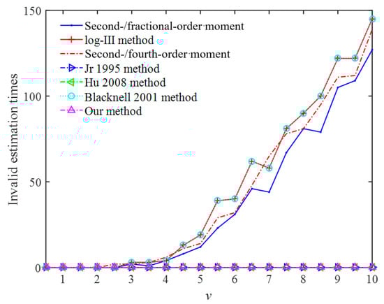
Figure 1.
The relationship between v and invalid estimation times in the data of the simulated K-distribution.
As can be seen in Figure 1, when , the invalid estimation times of all methods are 0. With the increase in , the invalid estimation times of references [18,26] and our method are still 0, and the invalid estimation times of the other methods are increasing.
When = 3 and the value of k is [0.1:0.1:3], the estimation efficiency of reference [26] and the proposed method can reach 100%, but the estimation accuracy of the proposed method is better. The relationship between k and the estimation accuracy of the RMSE is shown in Figure 2.
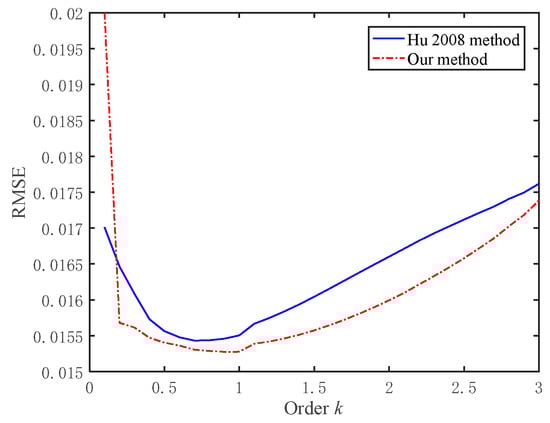
Figure 2.
The relationship between the order k and the RMSE in the data of the simulated K-distribution.
When k > 0.9, the RMSE will also increase with the increase in k. When k = 0.4, some simulation samples in the method of reference [26] begin to appear with a singular value, NaN, generated by the abnormal operation. When k = 2.9, the singular value NaN begins to appear in our method. The k is larger and the samples with singular values are greater. With the increase in k, the estimated value of in some samples will be relatively large, even greater than 100. When , Equation (1) will result in Inf/Inf, and NaN occurs. In Figure 2, the statistical result has eliminated the RMSE with a singular value. The larger the value k, the more samples will be eliminated.
The cumulative distribution function (CDF) can describe the statistical law of random variables and the tail of the K-distribution. For 1000 sets of simulation data with simulation parameters of = 3, = 1 and a sample length of 256 points, the CDF is used to further verify the fitting of each method to the trailing part of the K-distribution. Figure 3 shows the tail fitting of each method and the simulation data. According to the CDF fitting results, except for the method in [18], which has a poor tail-fitting effect, the other methods have a good tail-fitting effect. In general, the method in [18] has the worst performance, followed by the second-/fourth-order estimation method, the method used in [26], the log-III estimation method, and the method used in [27], and the second-/fractional-moment estimation method. The method in this study has the best performance.
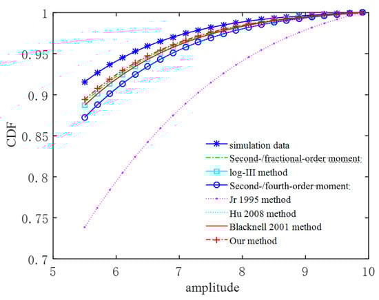
Figure 3.
The tail fitting of the K-distribution.
2. The measured data experiment. In order to further verify the effectiveness of the proposed method, 160 groups of the 256 points of measured IPIX data [19] are analyzed, and the parameters of the different methods are estimated, respectively. The IPIX data were collected on the shore of Lake Ontario in Grimsby, Ontario, Canada, including lake surface echoes on different days, at different times, and under different meteorological conditions. The measured data form is complex, including the I channel and Q channel, and the pulse repetition frequency is 1kHz.
The radar parameters are shown in Table 2.
Table 2.
The IPIX radar parameters.
The IPIX clutter data, which has a file name of 19980205_170935_ANTSTEP.CDF, includes 28 range units, with 60,000 scanning times. The 2D and 3D amplitude of the HH polarization is shown in Figure 4 and Figure 5, respectively.
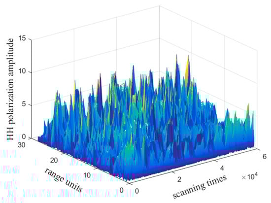
Figure 4.
Partial IPIX sea clutter 3D map of HH polarization.
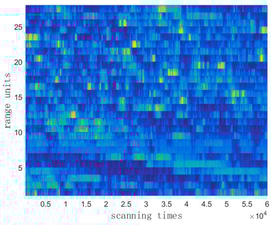
Figure 5.
Partial IPIX sea clutter 2D map of HH polarization.
The estimated effective rate is shown in Table 3.
Table 3.
The statistics of estimation efficiency and estimation accuracy in measured K-distribution (k = 0.5).
As can be seen from Table 3, the method in reference [18] has the worst performance. The performance of our proposed method is the best. The number of all effective estimated samples in this simulation experiment is 154 because there are 6 singular sample values NaN NaN in the method of reference [18]. The reason for generating singular values NaN has been explained previously.
In the measured IPIX data, when the value of k is [0.1:0.1:5], reference [26] and the proposed method can still reach 100% estimated efficiency, but the estimation accuracy of the proposed method is higher. The relationship between k and the RMSE is shown in Figure 6.
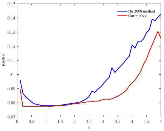
Figure 6.
The relationship between k and RMSE in the data of measured K-distribution.
When k > 0.9, the RMSE will increase with the increase in k. When k = 0.4, some simulation samples in the method of reference [26] begin to appear as the singular value, NaN, generated by the abnormal operation. When k = 4.1, the singular value NAN begins to appear in our method. The k is larger, and the samples with singular values are greater. When k = 5, 59 of the 160 samples have a singular value in the method of reference [26], more than 36%. When k = 5, 23 of the 160 samples have a singular value in our method, more than 14%. In Figure 3, the statistical result has eliminated the RMSE with a singular value.
We analyzed the calculation time of each method to illustrate the calculation complexity. Table 4 shows that the calculation time of the second-/fractional-order method is the minimum. This is because these methods use a special origin moment so that the gamma function is eliminated. The proposed method and the methods in references [18,26] contain the operation of the gamma function, but the calculation time of the proposed method is less than that in the methods of references [18,26].
Table 4.
The calculation time in simulated K-distribution (k = 0.5).
Through the experiments on the simulation data and measured data, it can be found that by selecting the appropriate order k, the estimation accuracy of the K-distribution can obtain a better value. It is necessary to select an appropriate estimation method according to the actual application.
3. The Extended Application of the Proposed Method
This method also can be applied to two-parameter models, such as log–normal distribution and Weibull distribution.
3.1. Log–Normal Distribution
The k-order origin moment of the log–normal distribution is shown in Equation (15):
The process of origin moment derivation is as follows:
Then, Equation (17) can be obtained from Equations (4) and (16).
Because:
By combining Equations (18) and (19), we can obtain:
Equation (19) can be further sorted into Equation (20).
Substituting the estimated value of the shape parameter into Equation (17), the estimated expression of the scale parameter can be obtained in Equation (21).
1. The simulated data experiment. The scale parameter is taken randomly in the interval between 0.5 and 0.9. The shape parameter is taken randomly in the range of −1.5 and −0.1. The MLE method [28], ME method [28], estimation method based on sample expectation and variance [29], and the proposed method are used for parameter estimation. The statistics of estimation accuracy of the RMSE are shown in Table 5.
Table 5.
The statistics of estimation accuracy in simulated log–normal distribution (k = 0.5).
Table 5 shows that the MLE and the proposed method have the highest estimation accuracy. In the simulation data, when the value of k is [0.1:0.1:3], the relationship between k and the RMSE is shown in Figure 7.
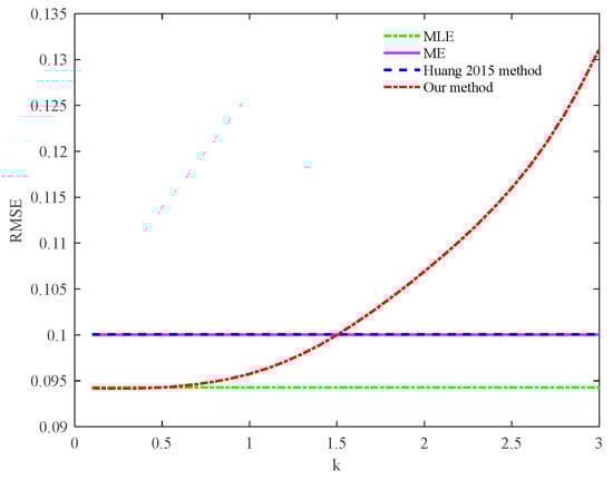
Figure 7.
The relationship between k and RMSE in the data of simulated log–normal distribution.
When k = 0.1∼0.4, the RMSE of the proposed method is smaller than that in MLE; When k = 0.5, the RMSE of the proposed method is the same as that in MLE, both of which are 0.0943. When k = 1.5, the RMSE of the proposed method is the same as that of the method in reference [29], both of which are 0.1000. When k > 0.4, with the increase in k, the RMSE will also increase. When k = 1.6, the RMSE exceeds the method in reference [29].
2. The measured data experiment. In order to further verify the effectiveness of the proposed method, 107 groups of measured IPIX data with a length of 256 points are modeled and analyzed, and the parameters of the different methods are estimated, respectively. The estimation accuracy of the RMSE is shown in Table 6.
Table 6.
The statistics of estimation accuracy in measured log–normal distribution (k = 0.5).
Table 6 shows that the proposed method has the highest estimation accuracy. In the measured data, when the value of k is [0.1:0.1:3], the relationship between k and the RMSE is shown in Figure 8.
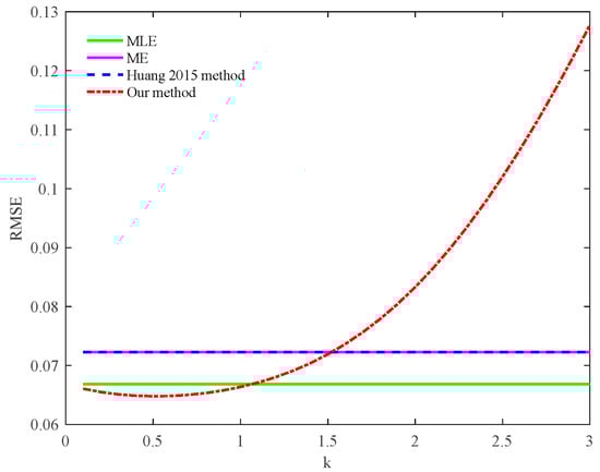
Figure 8.
The relationship between k and RMSE in the data of measured log–normal distribution.
When k = 0.1∼1, the RMSE of the proposed method is smaller than that in MLE; When k = 0.5 and 0.6, the RMSE has the minimum value of 0.0648. When k > 0.6, the RMSE will also increase with the increase in k. When k = 1.1, the RMSE of the proposed method exceeds the method in MLE.
We analyzed the calculation time of each method to illustrate the calculation complexity. Table 7 shows that the calculation time of the ME method is the minimum. The calculation time of the proposed method is longer than the other methods, but the calculation time is acceptable.
Table 7.
The calculation time in simulated log–normal distribution (k = 0.5).
Through the experiments, it can be found that when the value of k is 0.1∼1, the estimation accuracy of the log–normal distribution can obtain a better value.
3.2. Weibull Distribution
The k-order origin moment of the Weibull distribution is shown in Equation (22):
The process of the origin moment derivation is as follows:
Equation (24) can then be obtained from Equations (4) and (23):
It is found that taking the logarithm of can also obtain the term , that is:
By combining Equations (24) and (25), we can obtain:
Equation (26) is a nonlinear equation describing the shape parameter p. The estimated value of the shape parameter p can be obtained by solving Equation (26). We use the trust-region–dogleg [16] algorithm to solve the nonlinear equation. The complexity of the solution technology is provided in the following theoretical and experimental analysis. The estimated value of the shape parameter p is substituted into Equation (24), and the estimated expression of the scale parameter q can be obtained in Equation (27).
1. The simulated data experiment. The scale parameter is taken randomly in the interval between 0.3 and 3.2. The shape parameter is taken randomly in the range of 2.1–7.7. The MLE method [30], ME method [30], MENON estimation method [31], and the proposed methods are used for parameter estimation. The statistics of estimation accuracy of the RMSE are shown in Table 8.
Table 8.
The statistics of estimation accuracy in simulated Weibull distribution (k = 0.5).
Table 8 shows that the estimation accuracy of the proposed method is the highest. When the value of k is [0.3:0.1:4], the relationship between k and the RMSE is shown in Figure 9.
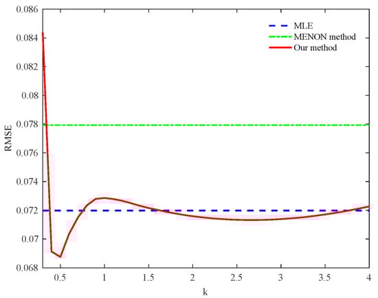
Figure 9.
The relationship between k and RMSE in the data of simulated Weibull distribution.
Through our analysis, when k = 0.4∼0.7 and k = 1.7∼3.7, the RMSE of the proposed method is slightly smaller than the MLE method. When k = 0.5, the RMSE has the minimum value of 0.0688.
2. The measured data experiment. In order to further verify the effectiveness of the proposed method, 100 groups of IPIX data with a length of 256 points are modeled and analyzed, and the parameters of the different methods are estimated, respectively. The estimation accuracy of the RMSE is shown in Table 9.
Table 9.
The statistics of estimation accuracy in measured Weibull distribution (k = 1).
Table 9 shows that the estimation accuracy of our method is the best. In the measured data, when the value of k is [0.3:0.1:4], the relationship between the RMSE and k is shown in Figure 10.
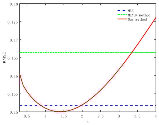
Figure 10.
The relationship between k and RMSE in the data of measured Weibull distribution.
When k = 0.9∼1.9, the RMSE of the proposed method is smaller than that of the MLE method. When k = 1.4, the RMSE has the minimum value of 0.1500. When k > 1.4, the RMSE will increase with the increase in k.
We analyzed the calculation time of each method to illustrate the calculation complexity. Table 10 shows that the calculation time of the MENON method is minimum. The calculation time of the proposed method is similar to that of the MLE method.
Table 10.
The calculation time in simulated Weibull distribution (k = 0.5).
Through the experiments using the simulation data and measured data, it can be found that the estimation accuracy of the Weibull distribution can obtain a better value by selecting an appropriate value of k.
4. Conclusions
Both the simulation and measured data experiments indicate that when the order k is an appropriate value, such as a smaller value, the origin moment derivation method can obtain an ideal estimation result and accuracy with a high probability. This conclusion is the same as that in reference [32], which points out that the high-order moment in the parameter estimation is sensitive to data, and the low-order moment should be selected as much as possible. The commonly used ME methods have the use of high-order moments, such as first-order, second-order, and fourth-order moments. These methods use different orders of k to solve simultaneous equations for convenience. The data are amplified using different orders, and the joint operation of different orders introduces different multiples of calculation errors. The derivation of the proposed method is based on a single order k; it will not introduce the error of different order operations. Thus, the calculation errors are smaller while the order k is an appropriate value. When k is given, the computational complexity of the proposed method is related to the PDF. The more complex the PDF, the greater the computational complexity, e.g., K-distribution and Weibull distribution contain complex gamma function and Psi function operations. The log–normal distribution has the operation of the square root. The proposed method is suitable for solving the parameter estimation problem in the form of the exponential function and the gamma function.
Author Contributions
Conceptualization, L.Y. and W.Y.; methodology, L.Y. and Y.L.; software, L.Y. and X.S.; validation, L.Y.; data curation, L.Y.; writing—review and editing, L.Y. and X.S.; supervision, Q.S.; All authors have read and agreed to the published version of the manuscript.
Funding
This work was supported by the National Natural Science Foundation of China (61921001, 61871384).
Data Availability Statement
Not applicable.
Conflicts of Interest
The authors declare there is no conflict of interest.
References
- Gong, M.; Cao, Y.; Wu, Q. A neighborhood-based ratio approach for change detection in SAR images. IEEE Geosci. Remote Sens. Lett. 2011, 9, 307–311. [Google Scholar] [CrossRef]
- Hakim, W.L.; Achmad, A.R.; Eom, J. Land subsidence measurement of Jakarta coastal area using time series interferometry with Sentinel-1 SAR data. J. Coast. Res. 2020, 102, 75–81. [Google Scholar] [CrossRef]
- Kang, M.S.; Baek, J.M. Efficient SAR imaging integrated with autofocus via compressive sensing. IEEE Geosci. Remote Sens. 2022, 19, 4514905. [Google Scholar] [CrossRef]
- Sayama, S.; Sekine, M. Amplitude statistics of ground clutter included town using a millimeter wave radar. IEICE Trans. Commun. 2003, 26, 829–836. [Google Scholar]
- Sayama, S.; Sekine, M. Log–Normal, Log–Weibull and K–distributed sea clutter. IEICE Trans. Commun. 2002, E85–B, 1375–1381. [Google Scholar]
- Ozgun, O.; Kuzuoglu, M. Physics-based modeling of sea clutter phenomenon by a full-wave numerical solver. Wave Motion Vol. 2022, 109, 102872. [Google Scholar] [CrossRef]
- Shao, Z.; Ji, W.; Qian, C.; Yang, Y. Ship detection for SAR images with sea clutter models estimation. In Proceedings of the 2021 2nd China International SAR Symposium, Shanghai, China, 3–5 November 2021; pp. 1–4. [Google Scholar]
- Greco, M.; Bordoni, F.; Gini, F. X–band sea–clutter nonstationarity: Influence of long waves. IEEE J. Ocean. Eng. 2004, 29, 269–283. [Google Scholar] [CrossRef]
- Chan, H.C. Radar sea—Clutter at low grazing angles. Radar Signal Process. IEEE Proc. 1990, 137, 102–112. [Google Scholar] [CrossRef]
- Walker, D. Doppler modelling of radar sea clutter. IEEE Proc.—Radar Sonar Navig. 2001, 148, 73–80. [Google Scholar] [CrossRef]
- Watts, S. Radar detection prediction in K–distributed sea clutter and thermal noise. Aerosp. Electron. Syst. 1987, 23, 40–45. [Google Scholar] [CrossRef]
- Lauritzen, S.; Uhler, C.; Zwiernik, P. Maximum likelihood estimation in Gaussian models under total positivity. Ann. Stat. 2019, 47, 1835–1863. [Google Scholar] [CrossRef]
- Du, X.; Liao, K.; Shen, X. Secondary radar signal processing based on deep residual separable neural network. In Proceedings of the 2020 IEEE International Conference on Power, Intelligent Computing and Systems, Shenyang, China, 28–30 July 2020; pp. 12–16. [Google Scholar]
- Abraham, D.A.; Lyons, A.P. Novel physical interpretations of K–distributed reverberation. Ocean. Eng. IEEE J. 2002, 27, 800–813. [Google Scholar] [CrossRef]
- Iskander, D.R.; Zoubir, A.M. Estimation of the parameters of the K-distribution using higher order and fractional moments. IEEE Transcations Aerosp. Electron. Syst. 1999, 35, 1453–1457. [Google Scholar] [CrossRef]
- Zhang, J.Z.; Xu, C.X. Trust region dogleg path algorithms for unconstrained minimization. Ann. Oper. Res. 1999, 87, 407–418. [Google Scholar] [CrossRef]
- Bellavia, S.; Macconi, M.; Pieraccini, S. Constrained Dogleg methods for nonlinear systems with simple bounds. Kluwer Acad. Publ. 2012, 53, 771–794. [Google Scholar] [CrossRef]
- Marier, L., Jr. Correlated K-Distributed clutter generation for radar detection and track. IEEE Trans. Aerosp. Electron. Syst. 1995, 31, 568–580. [Google Scholar] [CrossRef]
- Xu, X.H. Entropy metrics of radar signatures of sea surface scattering for distinguishing targets. Remote Sens. 2021, 13, 3950. [Google Scholar]
- Xu, W.; Chen, Y.S. An estimation method for K–distribution clutter parameters. Shipboard Electron. Count. Meas. 2013, 36, 82–84. (In Chinese) [Google Scholar]
- Tang, W.; He, H.; Gunzler, D. Kernel smoothing density estimation when group membership is subject to missing. J. Stat. Plan. Inference 2012, 142, 685–694. [Google Scholar] [CrossRef] [PubMed]
- Zhang, W.; Wen, A.; Wang, Q.; Li, Y.Y. Simple and flexible photonic microwave waveform generation with low RMSE of square waveform. IEEE Photonics Technol. Lett. 2019, 31, 829–832. [Google Scholar] [CrossRef]
- Ossant, F.; Patat, F.; Lebertre, M.; Teriierooiterai, M.L.; Pourcelot, L. Effective density estimators based on the K-distribution: Interest of low and fractional order moments. Ultrason. Imaging 1988, 20, 243–259. [Google Scholar] [CrossRef]
- Deng, Z.H. Statistical Modeling of Sea Clutter Based on Measured Data. Ph.D. Thesis, Xidian University, Xi’an, China, 2014. (In Chinese). [Google Scholar]
- Abraham, D.A.; Lyons, A.P. Reliable methods for estimating the K-distribution shape parameter. IEEE J. Ocean. Eng. 2010, 35, 288–302. [Google Scholar] [CrossRef]
- Hu, W.L.; Wang, Y.L.; Wang, S.Y. Estimation of the parameters of K–distribution based on zrlog(z) Expectation. J. Electron. Inf. Technol. 2008, 30, 203–205. (In Chinese) [Google Scholar] [CrossRef]
- Blacknell, D.; Tough, R. Parameter estimation for the K–distribution based on [zlog(z)]. IEEE Proc Radar Sonar Navig. 2001, 148, 309–312. [Google Scholar] [CrossRef]
- Bílková, D. Lognormal distribution and using L-moment method for estimating its parameters. Int. J. Math. Model. Methods Appl. Sci. 2012, 6, 30–44. [Google Scholar]
- Huang, C. Parameter estimation of the lognormal distribution. Stud. Coll. Math. 2015, 18, 19–20. (In Chinese) [Google Scholar]
- Bhattacharya, P.; Bhattacharjee, R. A study on Weibull distribution for estimating the parameters. J. Appl. Quant. Methods 2010, 5, 234–241. [Google Scholar] [CrossRef]
- Menon, M.V. Estimation of the shape and scale parameters of the Weibull distribution. Technometrics 1963, 15, 175–182. [Google Scholar] [CrossRef]
- Li, Q.L.; Yin, Z.Y.; Zhu, X.Q. Measurement and Modeling of Radar Clutter from Land and Sea; National Defense Industry Press: Beijing, China, 2017; pp. 262–265. (In Chinese) [Google Scholar]
Disclaimer/Publisher’s Note: The statements, opinions and data contained in all publications are solely those of the individual author(s) and contributor(s) and not of MDPI and/or the editor(s). MDPI and/or the editor(s) disclaim responsibility for any injury to people or property resulting from any ideas, methods, instructions or products referred to in the content. |
© 2023 by the authors. Licensee MDPI, Basel, Switzerland. This article is an open access article distributed under the terms and conditions of the Creative Commons Attribution (CC BY) license (https://creativecommons.org/licenses/by/4.0/).