Article

Impact of Climate Change Parameters on Groundwater Level: Implications for Two Subsidence Regions in Iran Using Geodetic Observations and Artificial Neural Networks (ANN)

by
Saeid Haji-Aghajany
1,2,
Yazdan Amerian
1 and
Alireza Amiri-Simkooei
3,*
1
Faculty of Geodesy and Geomatics Engineering, K. N. Toosi University of Technology, Tehran 1996715433, Iran
2
Institute of Geodesy and Geoinformatics, Wrocław University of Environmental and Life Sciences, Norwida 25, 50-375 Wrocław, Poland
3
Department of Geoscience and Remote Sensing, Delft University of Technology, P.O. Box 5048, 2600 GA Delft, The Netherlands
*
Author to whom correspondence should be addressed.
Remote Sens. 2023, 15(6), 1555; https://doi.org/10.3390/rs15061555
Submission received: 5 January 2023 / Revised: 3 March 2023 / Accepted: 9 March 2023 / Published: 12 March 2023
(This article belongs to the Topic Remote Sensing in Water Resources Management Models)

Abstract

:
This study aims to investigate how changes in meteorological indicators affect groundwater resources, and hence to predict groundwater levels using these indicators, particularly in regions experiencing drought and subsidence. Precipitation, temperature, evapotranspiration and precipitable water vapor (PWV) are important meteorological parameters to predict groundwater levels. Two subsidence areas with different weather conditions were selected to conduct a comprehensive study on the effect of temperature and precipitation on groundwater level changes. The correct locations of the two subsidence areas were determined by analyzing Interferometric Synthetic Aperture Radar (InSAR) images of Sentinel-1A using the small baseline subset algorithm. The interferograms were processed to correct tropospheric effects using the advanced integration method. Specifying the exact locations of the two areas, the meteorological parameters were downscaled using the Statistical DownScaling Model (SDSM), synoptic observations, meteorological data, and the General Circulation Model (GCM). An Artificial Neural Network (ANN) was then employed to predict the groundwater level changes as a function of meteorological data, including Global Positioning System (GPS)-based PWV and the evapotranspiration index. The trained ANN, along with the downscaled meteorological indicators, was used to predict groundwater level changes over two time periods. In the first period, the prediction was performed over the current years to investigate the performance of the method using the available data, whereas in the second period, the prediction was performed for the coming years, up until 2030. The results confirmed the high performance of the prediction algorithm, and the importance of including PWV and evapotranspiration in groundwater level predictions. The Pearson correlation coefficient was used to check the relationship between groundwater level changes and meteorological variables. The statistical significance of these coefficients was tested at the significance level α = 0.05 . In more than 80% of the cases, the correlation coefficients were statistically significant, reaching more than 0.70 in some of the months. It is also observed that an increase in the depth of groundwater level has an obvious relationship with an increase in temperature and a decrease in rainfall.

1. Introduction

Since the beginning of the Industrial Revolution, the increase in emissions of carbon dioxide, methane and other greenhouse gases has disturbed average weather conditions at global and local scales. Today, atmospheric levels of carbon dioxide have reached their highest levels in the last eight hundred thousand years [1]. Groundwater is considered an important resource, especially in arid and semi-arid regions, for reasons such as water potability, chemical composition, constant temperature, lower pollution coefficient and a higher level of reliability and sustainability in the water supply. The most important precipitation factors that affect nutrition, as a critical part of health and development, are the amount, distribution, intensity, duration and type of precipitation. For example, when the amount of precipitation exceeds the rate of evapotranspiration in a certain period, it is possible to feed the groundwater aquifer.
Many studies around the world have shown that temperatures are rising. Over the last 150 years, the average surface temperature in the Northern Hemisphere has increased by 0.76 degrees Celsius [2]. Since 1951, the average minimum and maximum temperatures in the world have almost doubled [3]. This increase in the average temperature has serious consequences for all biological and non-biological communities. Rising temperatures are also accompanied by a decrease in snow and ice cover, sea ice and mountain ice retreat, early spring in the Northern Hemisphere and an increase in the frequency of heavy precipitation events in the biological and physical indicators compatible with global warming [4]. Today, long-term changes in meteorological indicators studies are made possible by the output of GCMs and scenarios published by the Intergovernmental Panel. A review of past studies reveals the importance of these changes and their impact on water resources. Cohen examined the effect of precipitation and temperature change scenarios on precipitation and temperature and, consequently, changes in water levels in the Great Lakes of North America. The results showed that the water storage of large lakes will decrease in response to long-term changes in weather conditions [5]. Holman examined the effects of these changes and economic and social activities concerning groundwater recharge in the east of England and outlined solutions to its problems. The results showed that many factors such as changes in precipitation, changes in the thermal regime of coastal floods, urban development, forest lands and changes in cultivation and plowing can affect the future of groundwater resources [6]. Jykama and Sykes investigated the effects of weather changes on groundwater levels and of spatial changes on aquifer feeding in the basin Grand River in Ontario, Canada. The results showed that due to long-term changes in weather conditions, currents and feed volume of the aquifer increased [7]. Ng et al. reviewed the effect of these changes on groundwater recharge in the plains of northern Texas. The results showed that the amount of groundwater recharge will change between −75 to +35 percent [8]. Luoma and Okkonen studied the effects of future changes in weather conditions and rising Baltic Sea water levels on groundwater levels in southern Finland. The results showed that the groundwater recharge pattern has changed and that the seasonal effects of weather change on groundwater recharge will be in the form of floods in winter and droughts in summer [9]. Ertürk et al. evaluated the effects of current and long-term changes in weather conditions on groundwater resources in a small Mediterranean basin. According to the results, almost all components of the water balance have been reduced and water scarcity is expected to become an important issue in the future [10]. House et al. analyzed the impact of future weather changes on groundwater levels in a watershed in the United Kingdom. They concluded that due to changes in meteorological variables such as precipitation, temperature and evapotranspiration, the groundwater level decreases. In arid and semi-arid regions, groundwater is the main water resource for many applications. However, inappropriate use of groundwater reservoirs has caused the aquifers not to feed well. Therefore, it is important to study and predict the nutritional status of groundwater resources under the influence of weather change due to the fragility of these ecosystems [11]. Burgan checked the difference between ANN algorithms and Multiple Linear Regression for daily streamflow prediction [12]. Trabelsi et al. studied the effect of novel hybrid and benchmark machine learning algorithms to predict groundwater potentiality in drought areas [13].
The purpose of this paper is to investigate the relationship between meteorological parameters and groundwater depletion in subsidence regions. Iran is one of the countries that is severely facing the problem of declining groundwater levels. Iran, where groundwater is an important criterion for agricultural and urban-industrial development, is among the vulnerable countries in the field of water. A large number of shallow and deep wells have been drilled in the last few decades, resulting in the decline of the water table in aquifers. On the other hand, it has become apparent that groundwater prediction can help managers to manage groundwater resources. It is therefore important to study the causes of declining groundwater levels in different climate conditions within the country. In this research, we first use the InSAR technique to measure the subsidence in two study areas in Iran. Then, the meteorological indicators are downscaled and predicted on the subsidence center using the SDSM model and meteorological data. In the next step, the evapotranspiration and PWV parameters are computed based on the GPS observations. Unlike many studies, ignoring PWV and evapotranspiration, it is shown that these indicators have an important effect on a more accurate prediction of the groundwater level. The groundwater level is then predicted using an optimal ANN architecture. For this prediction, meteorological and groundwater level observations, along with PWV and evapotranspiration parameters, are considered as input to the training phase. The groundwater level prediction is performed over two time periods. In the first case, the prediction is performed for the current time so that the efficiency and accuracy of the method can fully be evaluated using the available observations. In the second case, the prediction will be made for the future. In both cases, the relationship between groundwater level changes and meteorological indicators will be investigated.

2. Background and Methodology

In the first step of processing, the subsidence points need to be carefully identified. Given that the weather conditions of the study area may result in a change in the subsidence signal position obtained from InSAR, a precise method should be used to eliminate the tropospheric effect in radar results and to obtain an accurate diagnosis of signals [14,15]. In the following, a detailed method to correct the tropospheric effect of InSAR measurements is described. After that, this section describes the downscaling and forecasting of climatic data as well as the neural network used to predict groundwater levels. We then show the required neural network data and how they are prepared. Finally, the results’ evaluation methods are presented.

2.1. Tropospheric Correction to InSAR Data

InSAR time series provides a powerful tool to detect surface displacement using a set of SAR acquisitions. The performance of this technique is affected by the accuracy and precision of the retrieved surface displacement and limited by the decorrelation of radar signals, phase-unwrapping error and atmospheric delay. Decorrelation is mainly caused by variations in the surface backscatter specifications over time and by the non-ideal acquisition strategy of SAR missions [16,17,18]. To overcome the problems related to the early SAR missions, including the large orbit separation between two acquisitions of the same track and the relatively long revisit time with non-regular images, two different types of InSAR time series techniques have been proposed: persistent scatterer and distributed scatterer algorithms. The persistent scatterer method uses phase-stable point scatterers. The distributed scatterer approach, which relaxes the strict limit on phase stability, includes regions that are affected by decorrelation through the exploitation of the redundant network of interferograms [19,20]. Based on the network of interferograms, the distributed scatterer methods can be divided into two categories: the first category uses the network of all possible interferograms [21] and the second category uses the network with small spatiotemporal baselines [22].
To reduce the tropospheric effect from the InSAR displacement field, both persistent scatterer and distributed scatterer algorithms traditionally rely on the spatiotemporal filtering of the phase by taking into account their different frequency specifications in the space and time domain [23]. Some of the previous studies used the empirical correlation between the tropospheric delay and topography [24]. Some new studies use atmospheric data, such as the Global Positioning System tropospheric delay and the Moderate Resolution Imaging Spectroradiometer [25,26], and some others use different approaches to estimate the tropospheric delay, such as 2D and 3D ray tracing as an advanced integration method based on meteorological data [27,28,29]. More information can be found in [30,31,32].
InSAR processes are performed using time delay and differential phase shift of radar acquisitions. When the radar signals propagate through the troposphere layers, their velocities are reduced, and the phase observations are affected due to spatial variations in tropospheric delays [33]. The tropospheric delay in the zenith direction is called the zenith tropospheric delay and is computed using the numerical integration as follows [33]:
Z T D = 1 0 - 6 { k 1 R d g m P ( z 0 ) + z 0 z ( ( k 2 - R d R v k 1 ) e T + k 3 e T 2 ) d z } k 1 = 0.776 K P a 1 , k 2 = 0.716 K P a 1 , k 3 = 3.75 × 10 3 K 2 P a 1
where z0 is the surface elevation, z is the highest altitude of the troposphere, Rv (461.495 Jkg−1K−1) and Rd (287.05 Jkg−1K−1) are the specific gas constants for water vapor and dry air, respectively, e is the water vapor pressure, P(z0) is the surface pressure, T is the temperature in K and gm is the averaged gravitational acceleration over the troposphere layer. To reduce the tropospheric effect from the radar phase, it is necessary to convert the zenith tropospheric delay to the line-of-sight direction. Based on the previous studies, this step is performed using a mapping function [29]. Using mapping functions can cause errors in the calculations and results. This error can even lead to a misdiagnosis of the displacement signal in the InSAR processing [29,34]. Therefore, in this study, an advanced but simple integration technique based on direct numerical integration on the line-of-sight direction is used to prevent errors related to the mapping function. As can be seen in Figure 1, this technique, like the simple integration method along the zenith direction, requires meteorological data in 3D space. The meteorological data on the signal path need to be determined using the interpolation approaches. In this study, the kriging and spline interpolations have been used in the horizontal and vertical directions, respectively [35]. More details about this technique can be found in references [29,34].

2.2. Downscaling and Long-Term Prediction

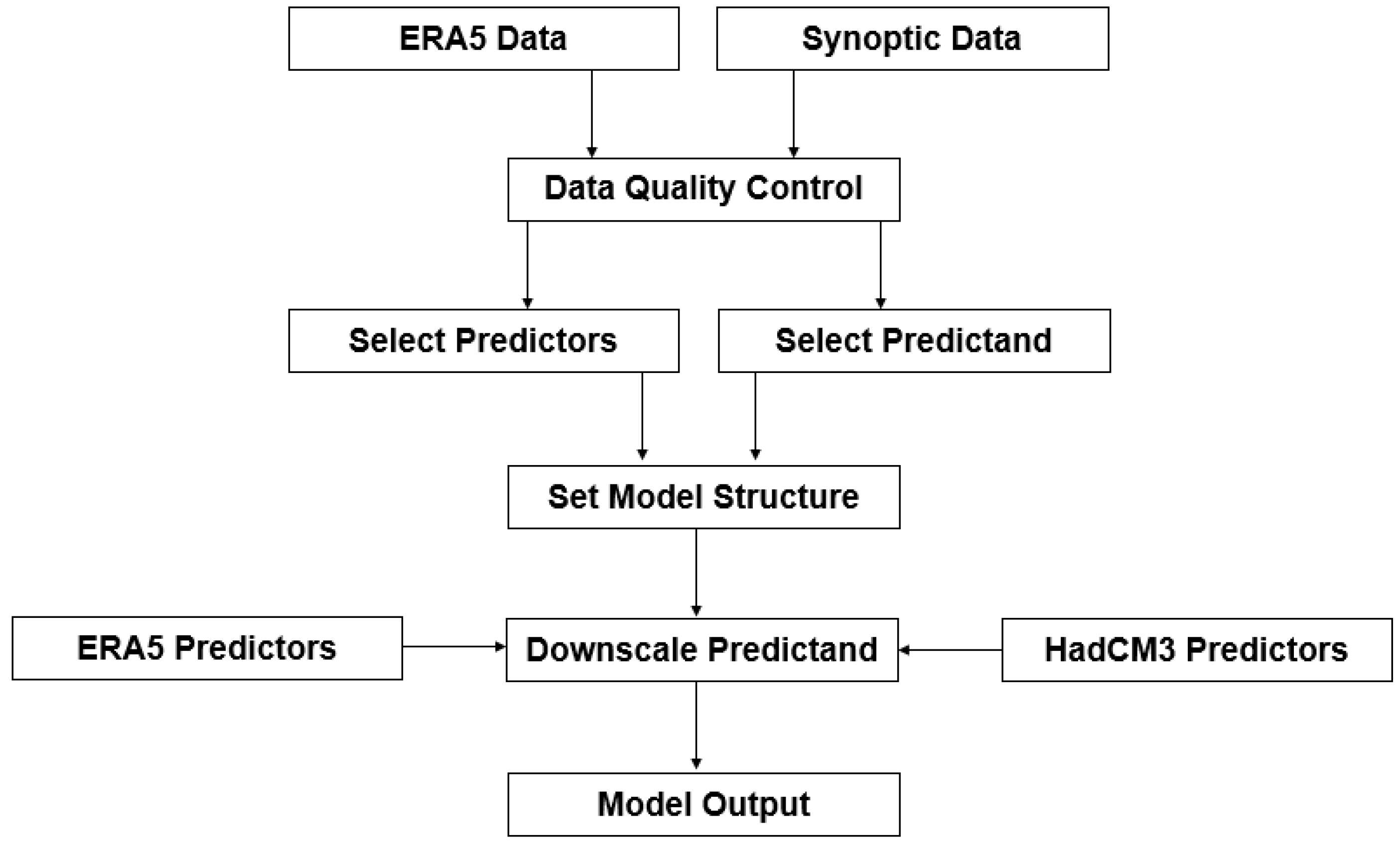
The SDSM model is used to downscale the meteorological data at a specific point in its current status and in future periods [36,37,38]. The input data of this model are time series of meteorological variables such as precipitation, minimum and maximum temperature and other atmospheric parameters. SDSM presents three different kinds of sub-models: monthly, seasonal and annual for the downscaling. The monthly sub-model is based on a special regression equation for each month, whereas the seasonal and annual sub-models generate one regression equation for each season and each year, respectively. In this study, the monthly sub-model type is preferred because of the large monthly variations in temperature and precipitation. In this mode, the SDSM generates different statistical parameters for each month. To produce and predict the data in the future, scenario A2 of the Hadley Centre coupled model-version 3 GCM [39], as well as ERA5 reanalysis data from the European Centre for Medium-range Weather Forecasts (ECMWF) along with the synoptic observations are used. Figure 2 shows the process of downscaling and production of the scenarios using SDSM.
The process of downscaling and predicting in this model consists of six steps. (1) Data gathering and quality control, (2) selection of appropriate predictor variables, (3) model training, (4) production of current meteorological data using observable variables, (5) statistical analysis of observed data, and (6) production of future meteorological data using the predictor variables [40].
It should be noted that there are three assumptions in downscaling and prediction of climate data:
      1-. Predictor and predictand data and their relationships are not affected by human-caused climate change and can be transferred to the next decades.
      2-. All downscaled parameters are obtained using the available data in the base period because it is assumed that, during the decades belonging to this time period, the data are of a higher quality and are more accessible than in other periods and, also, that the risk of instability in the relationship between predictor variables is small.
      3-. In climate simulations, it is assumed that the data follow the normal distribution.

2.3. ANN for Groundwater Level Prediction

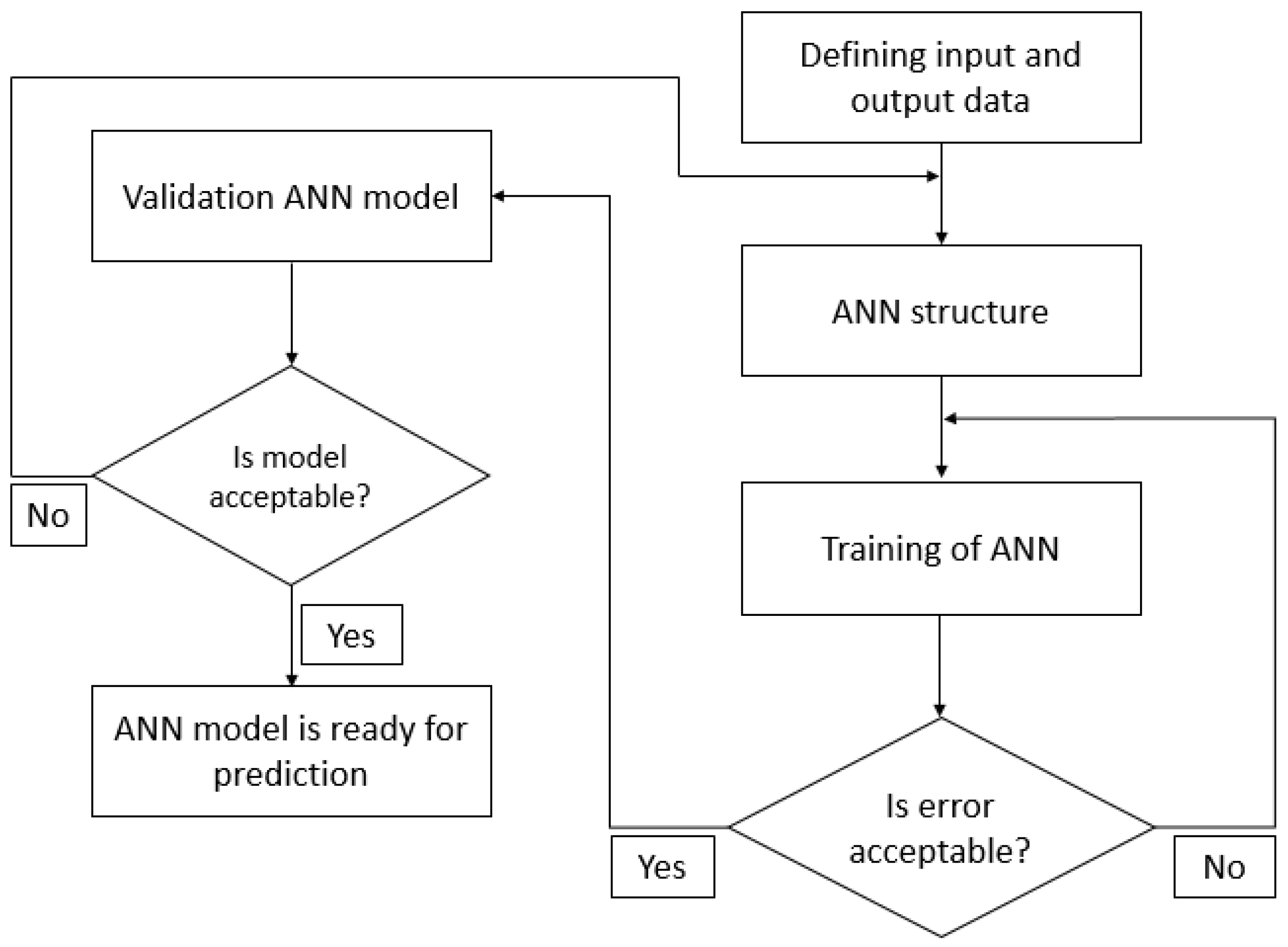
The ANN is a powerful and intelligent network that is known as a model for solving complex problems in various fields such as modeling, optimization, simulation, prediction and others. Figure 3 presents the steps of groundwater level prediction using ANN. The ANN model structure consists of three different layers: the input layer which receives data, the output layer which presents calculated outputs, and one or more hidden layers that work as the connection between the input and output layer [41]. A neuron is a basic processing unit of the ANN and performs two various operations: the reception of the inputs and the presentation of the output. The input data are prepared by connection weights and then passed through an activation function to present the output [42]. A multilayer feedforward ANN has neurons structured into layers and can pass in one direction without feedback connection. Multi-Layer Perceptrons (MLPs) are the most popular and the simplest state of ANN.
This class of approaches is widely used to create connections between the input and output data. MLPs are feedforward networks that include one or more hidden layers. MLP is a user-friendly method that gives a chance to determine any relationship between input and output data using the training algorithms. The Levenberg–Marquardt algorithm along with the Broyden–Fletcher–Goldfarb–Shanno, Gradient Descent and Conjugate Gradient Fletcher–Reeves Update methods have shown their strength and success in different ANN applications [38,41,42,43,44]. Among them, we selected the reliable and widely used Levenberg–Marquardt algorithm in order to perform the ANN training stage optimally. This method is a modified version of the classic Newton algorithm for computing a proper solution to the optimization processes [43,44].

2.4. PWV as a Key Indicator

One of the most important indicators that are often ignored in the groundwater level prediction process is PWV. GPS observations have been first processed using the BERNESE software [45]. The Zenith Total Delay (ZTD) and the tropospheric gradients have been computed at intervals of 1 and 4 h, respectively. The ZTD is equal to the sum of the Zenith Hydrostatic Delay (ZHD) and the Zenith Wet Delay (ZWD) [46,47]. The ZHD can be calculated from the Saastamoinen equation with acceptable accuracy [46,47]. In this study, GPS observations were used to compute PWV based on the following relationships [46,48,49]:
Z H D = 0.0022768 P 1 0.00266 cos ( 2 φ ) 0.00028 H
Z W D = Z T D Z H D
P W V = Π × Z W D = 10 6 ( K 3 T m + K 2 ) R V Z W D
where Π is the conversion factor, RV, K 2 and K 3 are constants with values of 461.50 (JK−1kg−1), 16.48 (KhPa−1) and 3.776 × 10⁵ (K2hPa−1), respectively, Tm (K) is the atmospheric weighted mean temperature, P is the surface pressure (hPa), and φ and H represent the latitude and the ellipsoidal height (km) of the GPS station, respectively.

2.5. Evapotranspiration Estimation

Evapotranspiration is another important parameter that helps estimate the amount of water needed for crops; it is crucial to correct irrigation planning. This parameter plays an important role in groundwater level prediction; therefore, it is considered an important input in ANN for groundwater level prediction. Because this index is not directly available to the users, it is necessary to determine its values by the experimental relationships. The Food and Agricultural Organization-proposed Penman–Monteith (PM) equation is the most popular equation to estimate evapotranspiration [50]:
ET ( P M ) = 0.408 ( R n G ) + γ 900 T a + 273 U 2 ( e s e a ) Δ + γ ( 1 + 0.34 U 2 )
where ET is evapotranspiration, G is soil heat flux density, Rn is net radiation at the crop surface, Ta is the mean daily air temperature at 2 m height, es is saturation vapor pressure, U2 is the wind speed at 2 m height, ea is actual vapor pressure, ∆ is slope vapor pressure curve and γ is psychrometric constant. It should be mentioned that this parameter is not equal to groundwater evapotranspiration. Due to the dependence of this relationship on a large number of meta-indicators that are often not published by databases or are accessible with different temporal and spatial resolutions, the use of this relationship is usually difficult. Unlike the PM equation, the TH method can estimate the amount of evapotranspiration based on air temperature [51].
ET ( T H ) = { 0 T 0 16 K ( 10 T l ) m T > 0
where l and m are the heat factor and coefficient, respectively, and K is the calibrated coefficient of latitude and month. Due to the sensitivity and importance of this index and its role in predicting the groundwater level, it was necessary to calculate this index with the utmost possible accuracy. For this reason, a new method based on GPS observations has been used in this study [52]. In this method, the evaporation index value based on the PM method is considered as an accurate model. The aim of this algorithm is to model the difference between the PM and TH methods over time by using water vapor obtained from GPS, as well as temperature. Finally, the modeled difference should be added to the TH formula to correct it. DET can be modeled using a linear equation based on the temperature and water vapor:
D E T = E T P M E T T H
D E T = { a 0 × P W V 1 + a 1 × T + a 2 T 0 b 0 × P W V 2 + b 1 × T + b 2 T < 0
where a0a2 and b0b2 are the model coefficients, which can be determined based on the least squares method. PWV1 and PWV2 are the PWV at the moment of T 0 °C and T < 0 °C, respectively. Finally, the more accurate value of the evapotranspiration index can be calculated using the following equation:
E T A c c u r a t e = D E T + E T T H
Therefore, the ETAccurate can be computed at different times based on the differential model and without dependence on many meteorological indices. If there is a need to calculate this index as a two-dimensional map, it is also possible to enter the geographic location into the fitted model. Considering that it is necessary to calculate this index at the location of the station, the differential model is considered only in time. More information about how to use the differential model in temporal and spatial dimensions can be found in [52].

2.6. Effective Rainfall

Agriculture is one of the most important reasons for groundwater consumption and hence the reduction in its level. This variable should be considered in groundwater level prediction. In other words, to investigate the impact of meteorological parameters on the groundwater level, it is necessary to calculate the amount of water consumed through agriculture and consider it in the prediction process. The amount of consumed water is achievable according to the statistics provided by the water organization of each country. Based on the relationship between the amount of water consumed in agriculture and the effective rainfall (ER) index, it is possible to predict the amount of consumed water in the future. In this contribution, this value is removed from the prediction process. In this case, the final changes in the groundwater level can only be considered as a result of changes in meteorological parameters. The ER is estimated by different methods, such as the ratio method. The approximation is based on the properties of soil and runoff, and dryness also plays a role [53]:
E R = E T P
where ET is evapotranspiration and P is rainfall. In this paper, the information provided by the Iranian Meteorological Organization (IMO) and the Iranian Geological Organization (IGO) has been used to correct the effect of consumed water.

2.7. Validation Methods

The statistical indicators, namely, the Root Mean Square Error (RMSE), Nash–Sutcliffe efficiency (NSE) and the coefficient of determination (R2) have been used to compare and validate the results [54]. The Pearson correlation coefficient was used to determine the correlation between water level changes and meteorological indicators. In addition, the significance of the estimated correlation coefficient is determined based on the given confidence interval. The statistical tests have a null hypothesis. For most tests, the null hypothesis is that there is no relationship between your variables of interest or that there is no difference between groups.
Null hypothesis (H0): there is no significant difference between the two sets of data
Alternative hypothesis (H1): there is a significant difference between the two sets of data
The p-Value is a number, calculated from a statistical test, that describes how likely you are to have found a particular set of observations if the null hypothesis were true. p-Value is used in hypothesis testing to help decide whether to reject the null hypothesis. The smaller the p-Value is, the more likely you are to reject the null hypothesis. p-Value is most often used by researchers to say whether a certain model they have presented is statistically significant. Statistical significance is another way of saying that the p-Value of a statistical test is small enough to reject the null hypothesis of the test [54]. The threshold considered in this study is p-Value < 0.05. In other words, this test is performed at a significance level of α = 0.05.

3. Study Area and Data Set

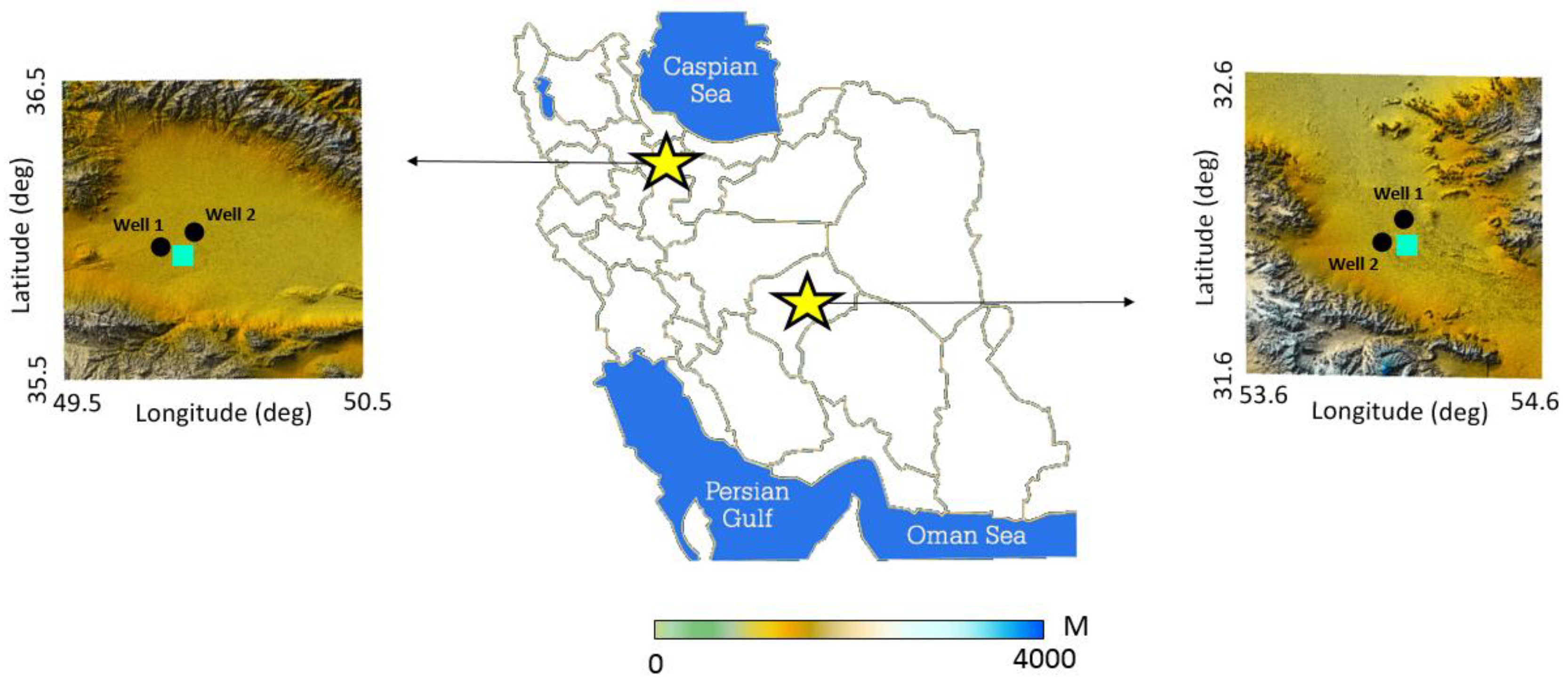
Iran is a country with different weather conditions in different regions, and, in recent years, it has faced severe subsidence due to declining groundwater levels. Two regions with different weather conditions are selected in Iran. The first study area is part of the Qazvin plain with mountainous weather conditions and the second area is part of the Yazd plain with hot and dry weather. The location of the study areas can be seen in Figure 4. According to the statistics provided by the United Nations, Iran’s population is currently 86,022,843, which will increase by 3% in 2030 [55]. According to the information provided by the Statistical Center of Iran, the study areas of this research have the lowest population growth rate in Iran. These two areas are also outside urban areas, and increased personal consumption due to population increase has the least impact on the groundwater level. However, by employing the existing algorithm, the use of groundwater due to population changes has also been removed from the observations [56]. This includes, for example, the effects related to agricultural uses. Therefore, the results can be attributed to meteorological indicators.
The average precipitation and temperature in these two regions are different and this difference provides the basis for a detailed investigation. Figure 5 and Table 1 show the difference between precipitation and temperature in the center of these two regions. These two meteorological parameters show visible variations in the two study areas.
In this study, three types of meteorological data are used. The first type is the daily meteorological data from synoptic stations that are used for the training and evaluation step. The second type of meteorological information is the ERA5 reanalysis data from ECMWF that have been used as large-scale data for training. The tropospheric correction of the InSAR observations is also performed using the ERA5 reanalysis data from ECMWF. It presents values of the meteorological information on 37 pressure levels, and with a spatial resolution of about 31 km from 1950 to the present [57]. Based on the previous investigations, the reanalysis data are useful and practical in different applications such as geodesy, meteorology, remote sensing and geodynamics. The third type is the Hadley Centre coupled model-version 3 GCM information based on different scenarios that have been used for meteorological data prediction. This model presents different parameters such as temperature, humidity and wind speed. This model has 19 levels with a horizontal resolution of 3.75 degrees longitude and 2.5 degrees latitude. This is equivalent to the Earth’s surface resolution of about 417 km × 278 km at the Equator, reducing to 295 km × 278 km at 45 degrees latitude [39].
Based on the aim of this study, the InSAR technique has been used to identify the exact location of the subsidence signal. To implement the InSAR technique, a number of Sentinel-1A radar acquisitions taken from these two areas have been used. The radar images have been provided by the European Space Agency (ESA). The specifications of radar images can be seen in Table 2.
Groundwater level observations from the existing wells have also been used to calibrate and validate the ANN and, therefore, to predict groundwater level changes. The groundwater level data and needed information such as groundwater consumption have been prepared by Iranian regional water companies, IMO and IGO. Some of the statistical properties of groundwater level data can be seen in Table 3. GPS measurements obtained from the existing stations in both study areas have been used to estimate PWV and ET.

4. Processing Results and Discussions

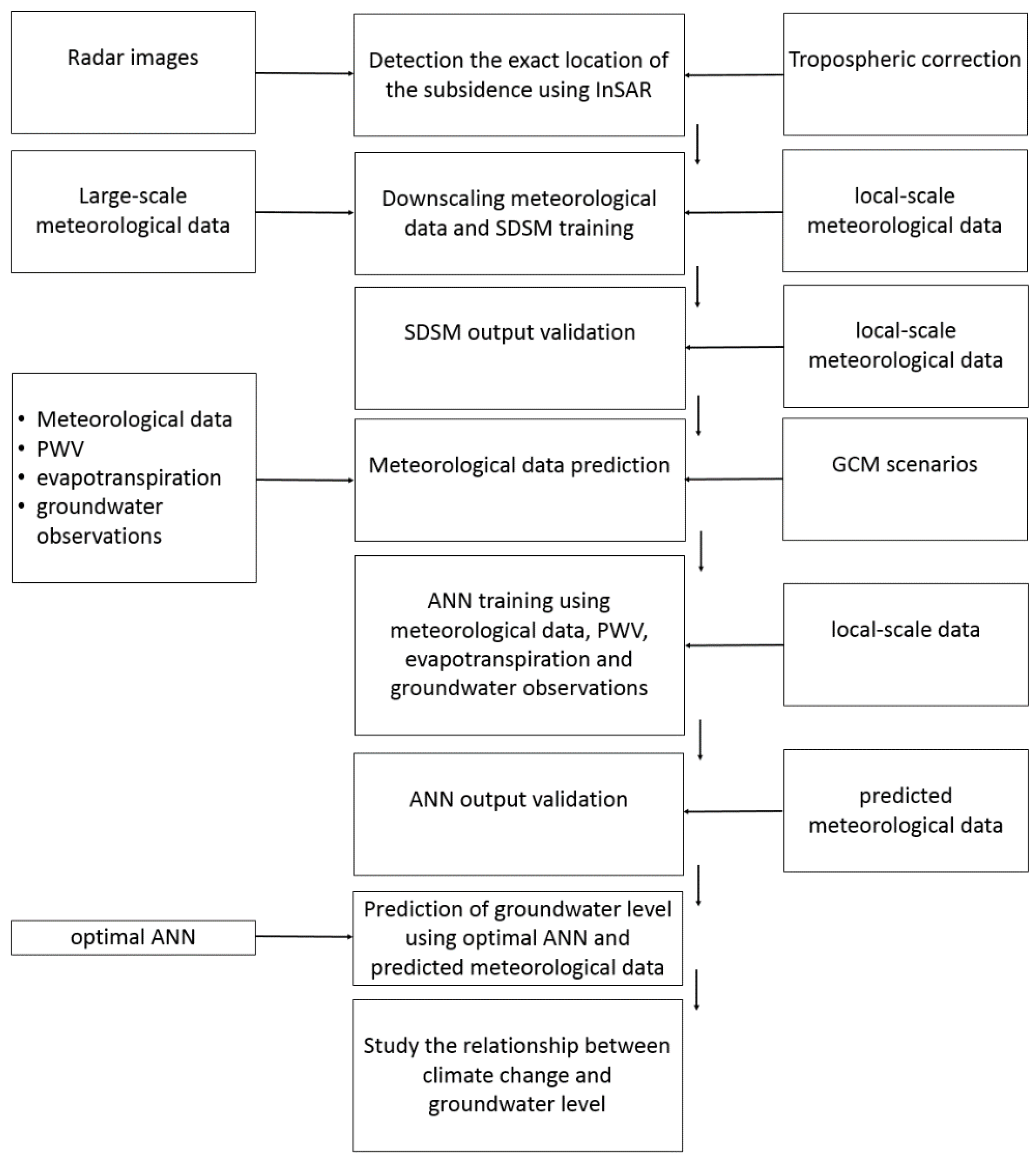
Figure 6 presents the processing steps to study the relationship between changes in meteorological indicators and groundwater levels.
In the first step, it is necessary to determine the subsidence area using InSAR. After determining the subsidence zone, SDSM is trained using large-scale and local-scale meteorological data. Then, using the local meteorological observations, the trained model is validated, and finally, the values of the temperature and precipitation are downscaled to the location of the desired stations. The meteorological parameters, in the future, will then be predicted using SDSM. In the next step, it is necessary to select the optimal ANN parameters to predict the groundwater level in the future. The meteorological data, along with groundwater observations, are then considered as input to the training phase. The trained ANN is evaluated using local observations, and the optimal ANN specifications are selected. The groundwater level is then predicted. Finally, the relation between the temperature and precipitation changes and the groundwater level can be studied.

4.1. Subsidence Detection

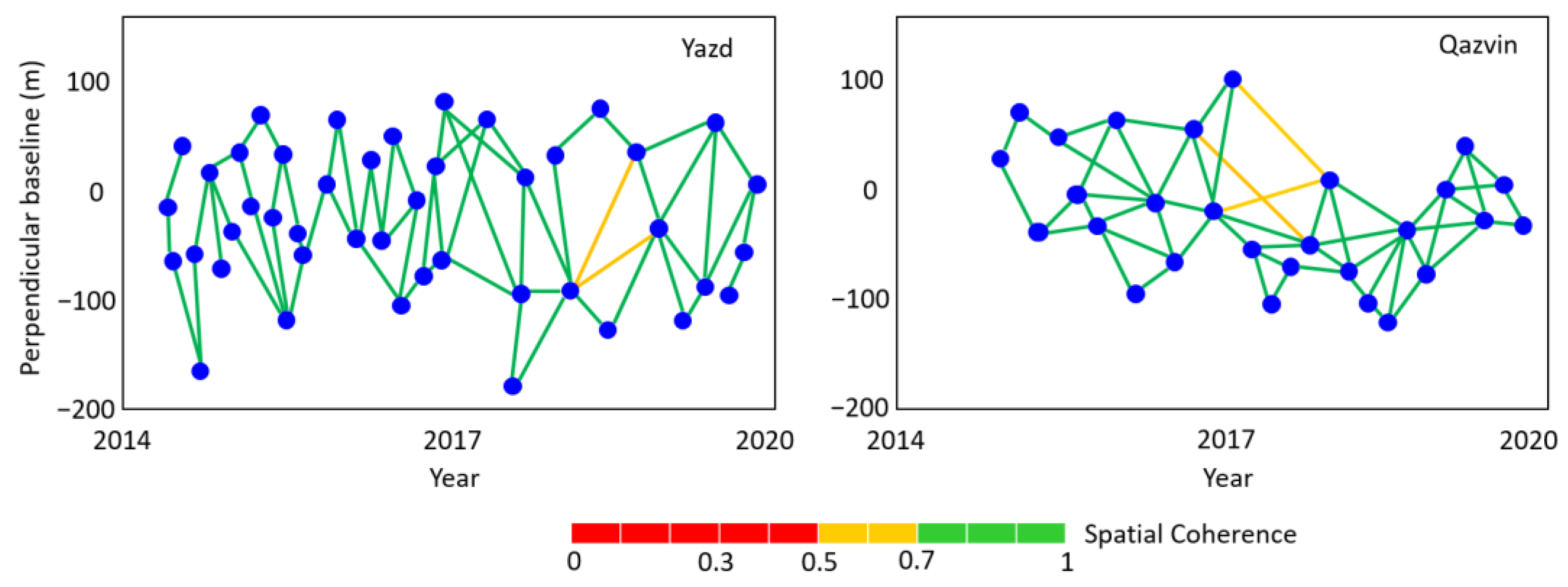
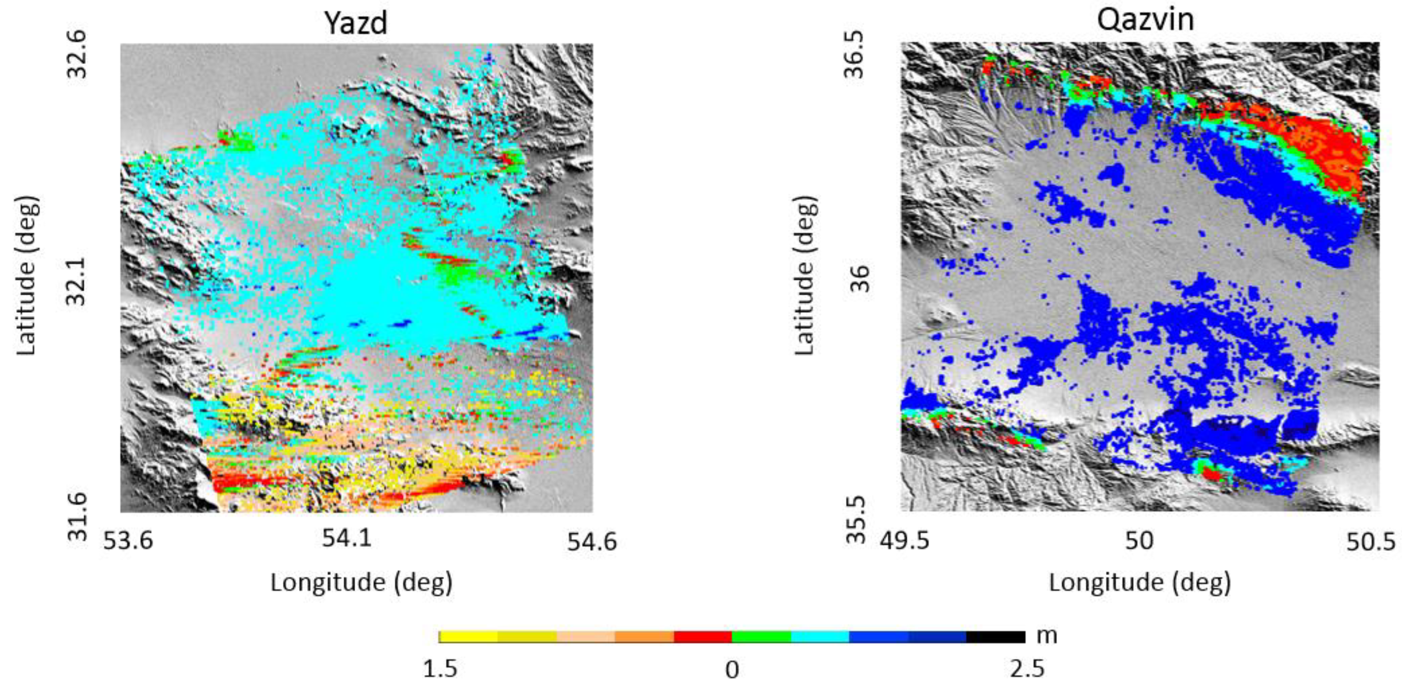
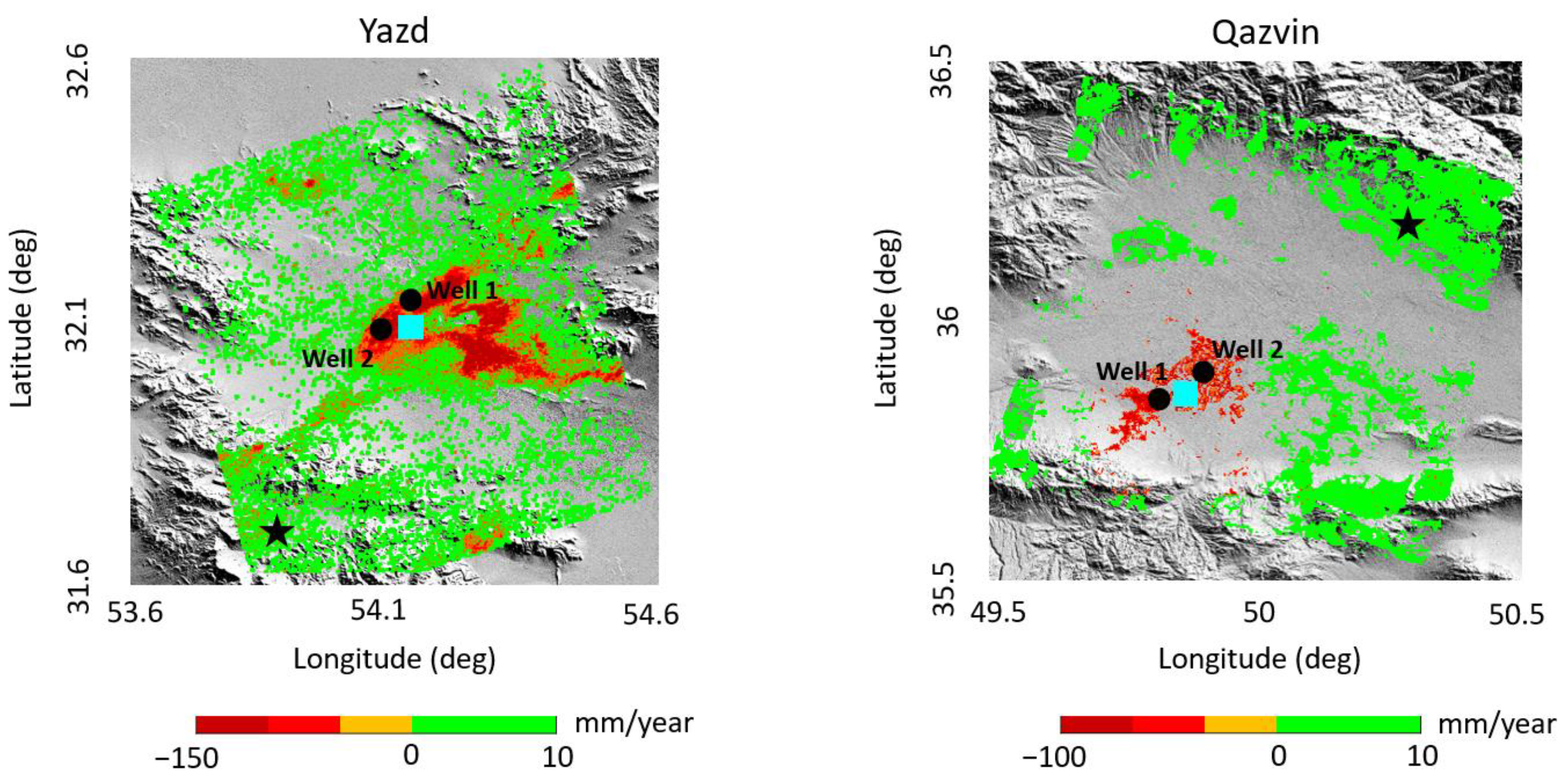
A number of Sentinel-1A radar acquisitions have been used to perform the InSAR analysis. In this process, the Amplitude Dispersion Index has been selected to be 0.42. First, the interferograms were selected according to their spatial coherence (Figure 7). In addition, a reference point has been selected with respect to the smallest phase variance and the maximum of coherent pixels. In order to compute the displacement velocity, disturbing effects must be removed from the obtained interferograms. After removing the disturbing parameters using the Digital Elevation Model and orbital data, the interferograms only contain tropospheric effects and the displacement phase. The tropospheric effect was estimated using the advanced integration method and applied to the interferograms. An example of the obtained tropospheric delay can be seen in Figure 8. Finally, the displacement velocity map was calculated using the small baseline subset method. Figure 9 shows the obtained displacement velocity for the two study areas.
The computed displacement velocity in the Yazd region indicates a subsidence signal at the center of this area. The amount of the subsidence reaches 150 mm/year, which is considered to be a high and dangerous rate. There is no significant displacement in other parts of the area. In the Qazvin area, the subsidence signal is clearly visible. The maximum subsidence rate is 100 mm/year. According to the location of the subsidence signals in both areas, the local groundwater observations, as well as the synoptic station, have been selected.

4.2. Downscaling and Prediction of Meteorological Parameters Using SDSM

The processing of this paper takes place over two periods of time. In the first period, the purpose is to predict the groundwater level between 2013 and 2020 so that the results and methods can be fully evaluated using the available observations. The second mode is making predictions for the future, between 2021 and 2030. Therefore, the prediction of meteorological indicators has also been conducted in two time frames. In the first case, the data between 1985 and 2010 have been used for training and the data between 2011 and 2012 were used to evaluate the model. In addition, the data between 1985 and 2018 have been used for training and the data from 2019 to 2020 were used to evaluate the predictions made for meteorological indicators. The comparison results between the downscaled mean monthly temperature and precipitation and their observed values, in terms of the above-mentioned statistical measures, are provided in Table 4 and Table 5.
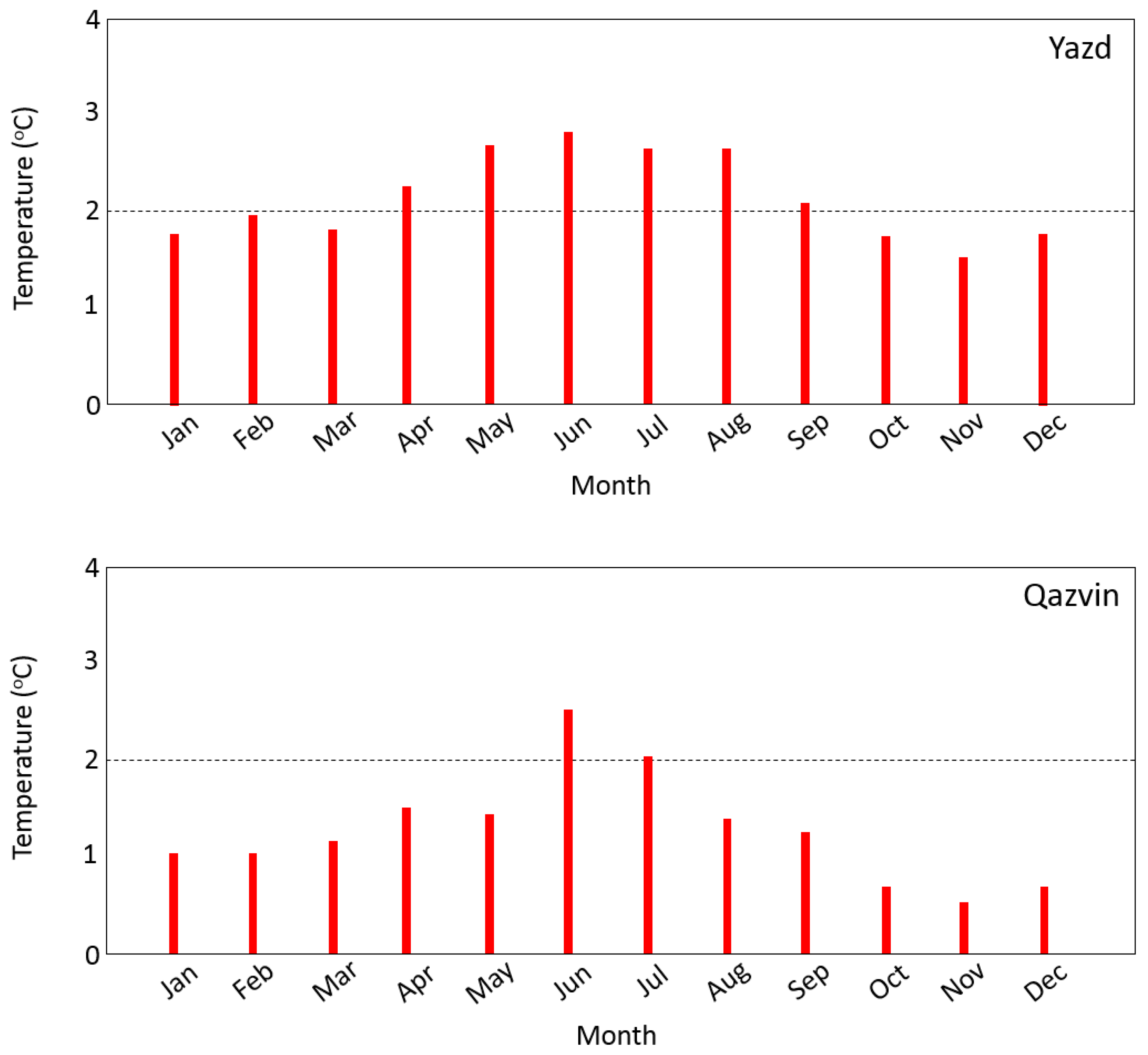
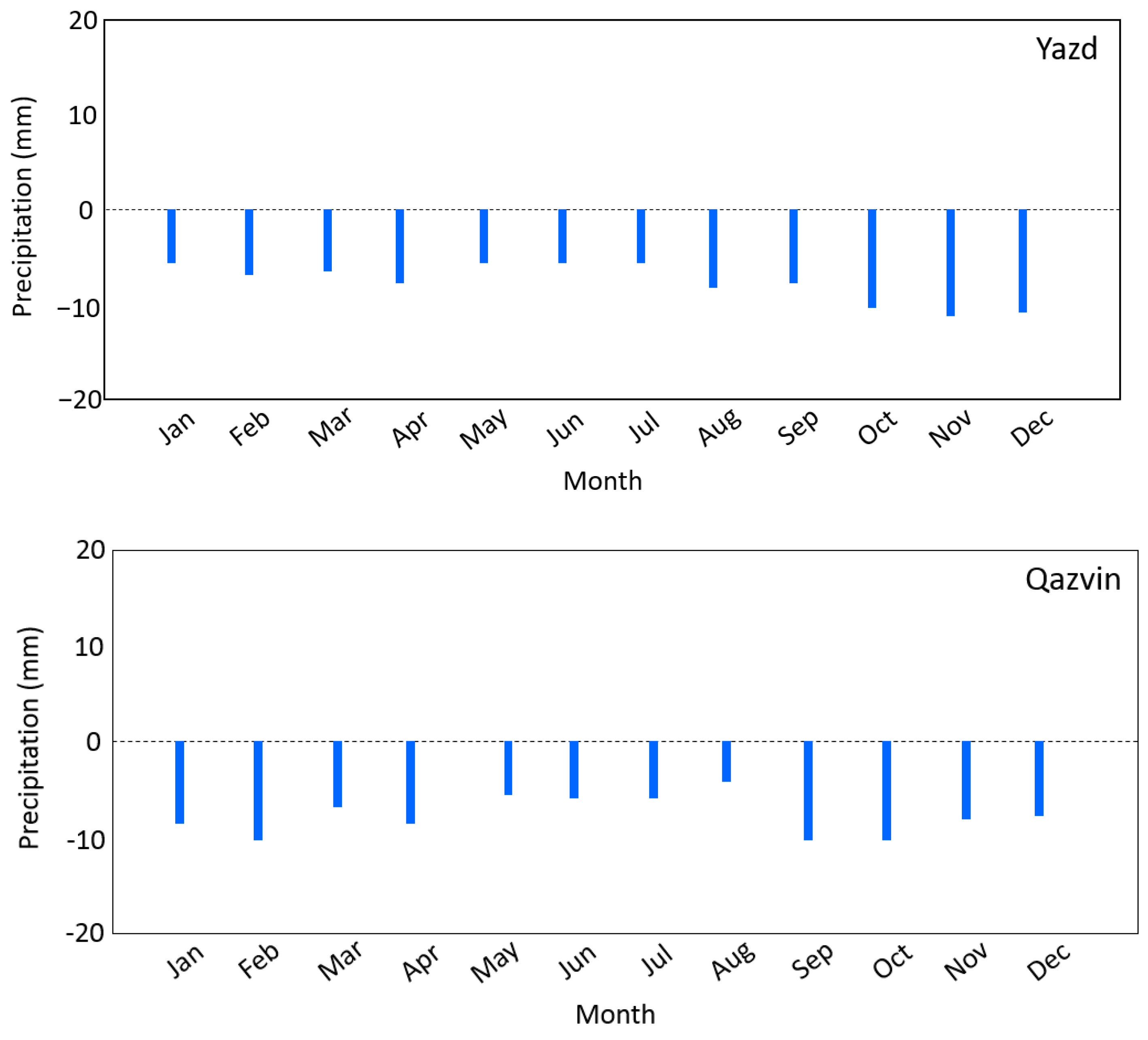
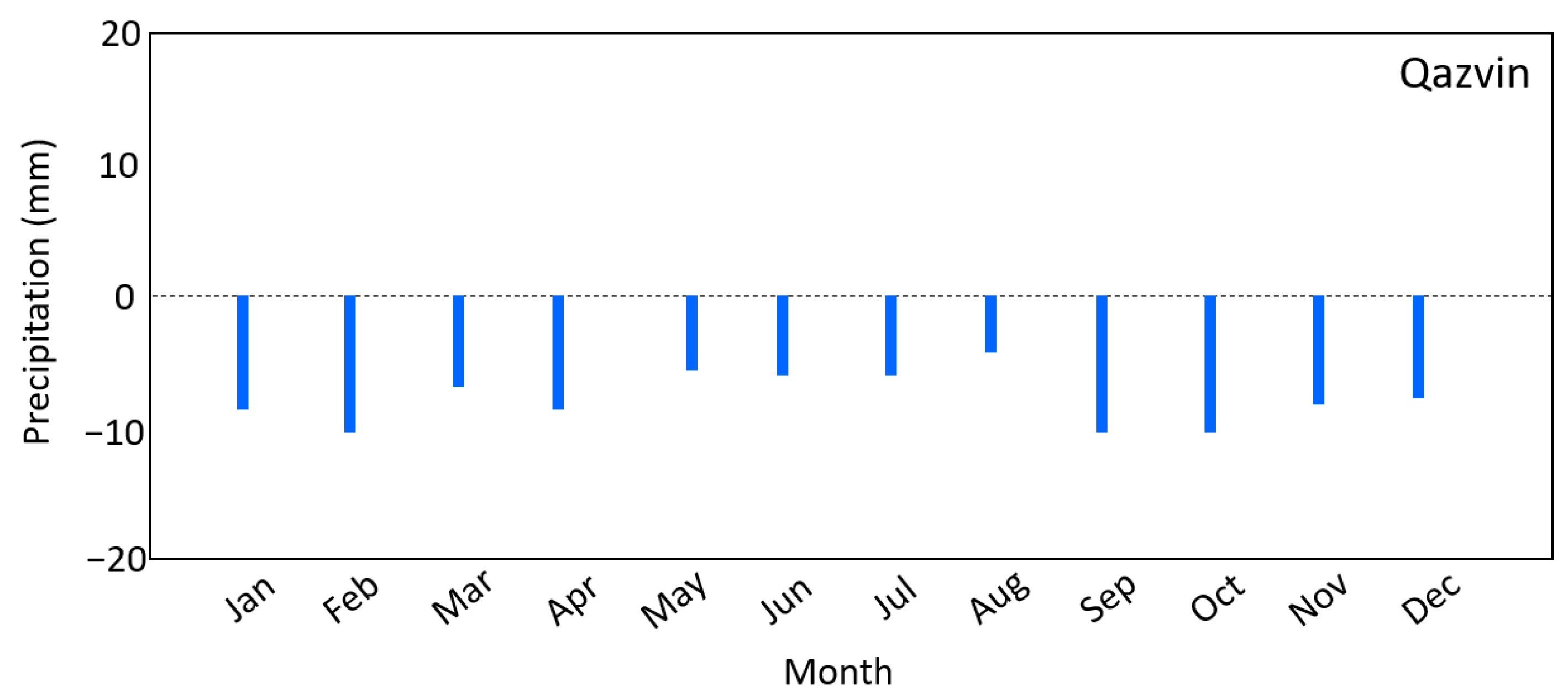
Finally, using the downscaled data as well as the produced scenario, the values of meteorological parameters in the time span of 2013 to 2020 have been predicted. Figure 10 and Figure 11 show the monthly average of predicted meteorological variables in the time span of 2013 to 2020 compared to the base period. According to the prediction, the temperature in both regions will increase in the coming years. This increase is more noticeable in the warmer months of the year. In the Yazd region, the maximum temperature changes, compared to the base period, are about 3 degrees for the years 2013 to 2020. In the Qazvin region, the maximum rate of temperature increase, compared to the base period, is about 2.5 degrees. The results of precipitation prediction show that this parameter will decrease in the coming years and that this decrease is more significant in the cold months of the year. The biggest decreases for the Qazvin region in this period will occur in January, September and November by about 9 mm. After predicting the meteorological parameters and computing the ET and PWV, we can now predict the groundwater level changes using the ANN, which we will show in the next section.

4.3. Groundwater Level Prediction from 2013 to 2020

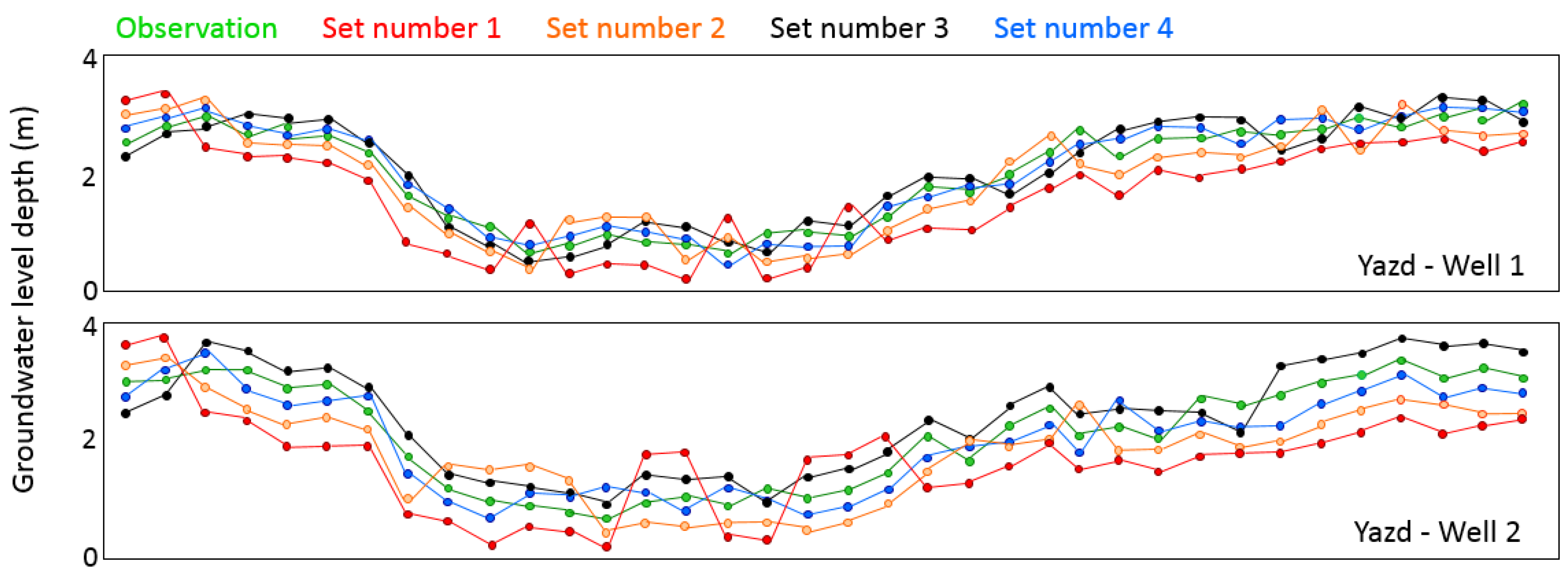
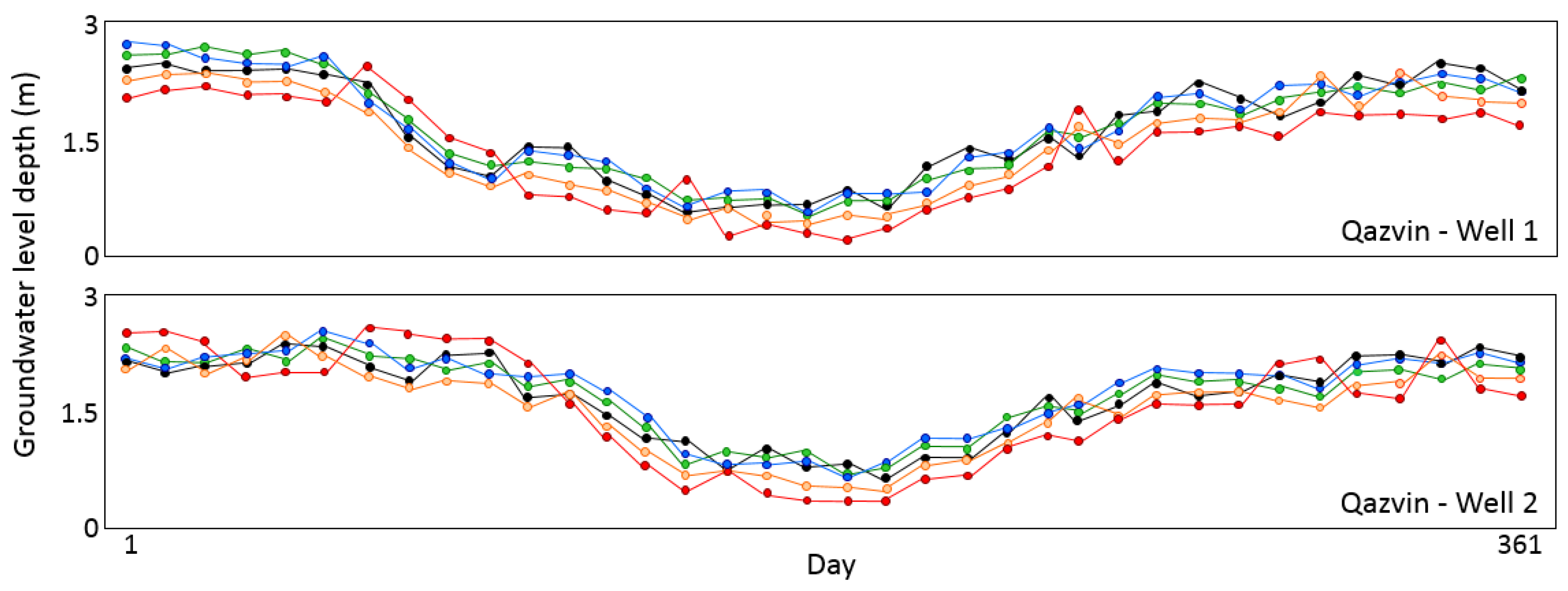
In order to check the effect of the use of PWV and ET and the statistical evaluation of all the mentioned processes, the prediction period is considered between 2013 and 2020. In this case, using the available observations, a comprehensive statistical evaluation of the method can be provided. In the first step, it is necessary to select an optimal ANN setting. The optimal ANN is organized to predict groundwater level changes. Based on the previous studies, the Levenberg–Marquardt algorithm has been selected as the most appropriate training function. The sigmoid log and hyperbolic tangent activation functions have been used for the hidden layers, and the linear activation function has been selected for the output layer. To determine the impact of PWV and ET on the prediction process, various input sets have been used to train the ANN. Table 6 shows different types of input parameter sets for the ANN to predict groundwater levels. These parameters generally include precipitation, Tmin, Tmax, groundwater level depth, PWV, ET and Solar Radiation (SR). Based on the algorithm, the ANN has been launched using different sets of inputs. In this process, 80% of the data are used for training and the remaining 20% are considered for validation. Figure 12 shows the comparison between the observations and the simulated changes in the groundwater level from different input sets. RMSE of different modes obtained from the validation step can be seen in Table 7.
The RMSEs show that data set No. 4 is the optimal ANN to predict groundwater level changes. These comparisons show that the use of PWV and ET obtained from GPS measurements leads to an increase in prediction accuracy. As it can be seen, when PWV and ET are not used (set 1), in addition to creating large errors, it also leads to a change in the trend of the graph in some parts. The biggest difference between the results obtained from data set 1 and the observations can be seen in the warmer months of the year. This is because, in the warmer months, PWV and ET play more important roles in the calculations than in the colder months. The results show that ANN with input set number 4 has a high ability to simulate the groundwater level in both areas and provides a reliable tool in predicting these variations in the coming years.
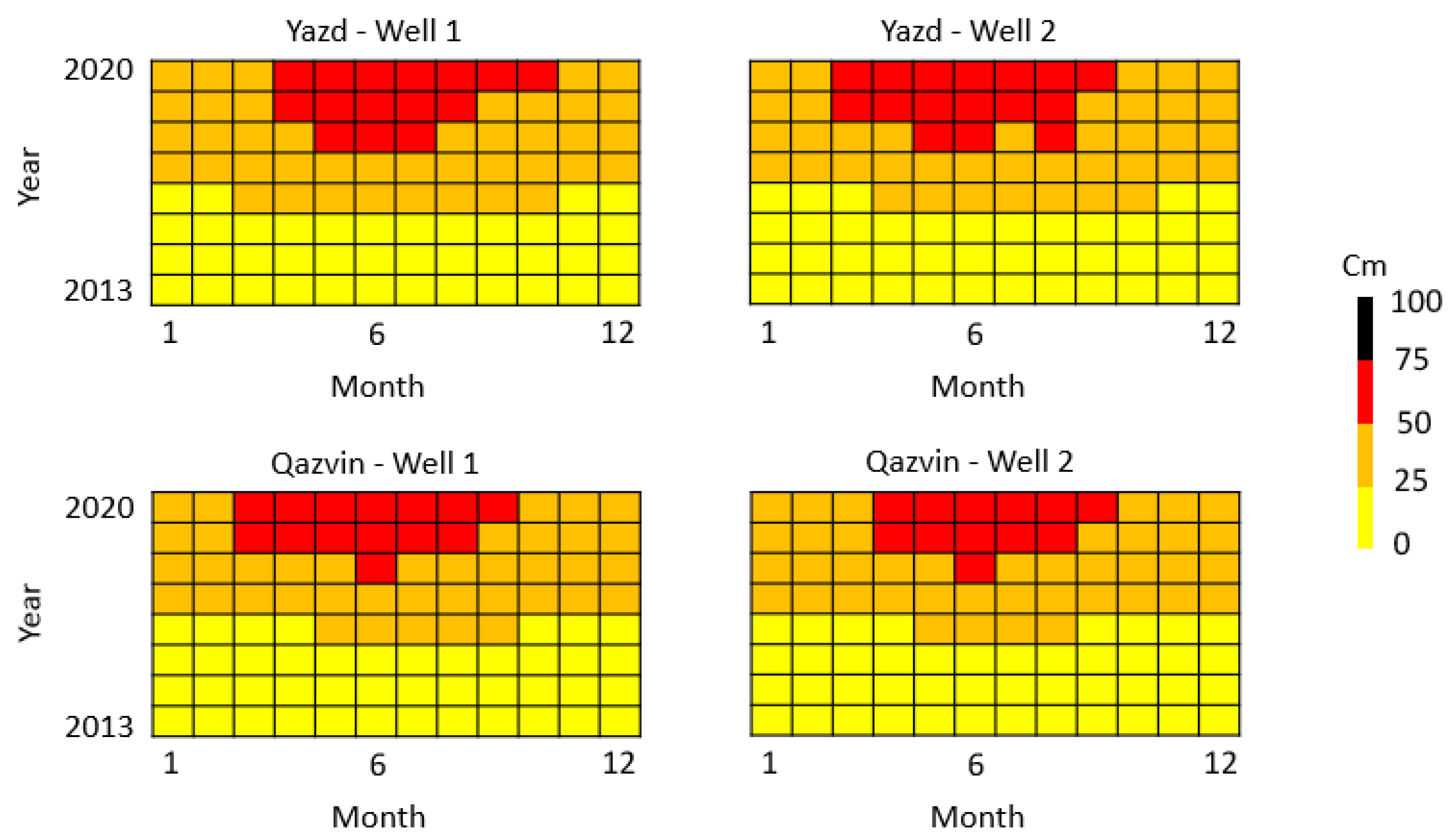
After checking the accuracy of the algorithm, in this step, the relationship between the time variations in temperature and precipitation and groundwater level changes is investigated. For this aim, the heatmap plot of the monthly average of groundwater level depth changes according to the baseline period is visible in Figure 13. Based on Figure 13 it can be concluded that most of the variations occurred in the warmer months of the year. After 2015, the process of increasing the groundwater level depth compared to the base period has become faster. This amount reached more than 50 cm in July and June 2020. This trend is evident in both study areas and it can be considered a result of a decrease in precipitation and an increase in temperature. The lowest number of changes are related to the beginning and end months of the year, which can be attributed to fewer changes in meteorological indicators compared to the warmer months of the year. The statistical results related to the comparison between the monthly averages of predicted groundwater level changes and temperature and precipitation changes can be seen in Table 8.
In Table 6, two items are considered: first, the Pearson correlation coefficient, and second, the significance of the computed correlation using p-Value. It should be noted that this test has been conducted at a significance level of 0.05. As can be seen, the correlation coefficient between water level depth changes and meteorological indicators reaches 76%. As expected, this correlation is positive for the precipitation index and negative for the temperature index. In fact, with the increase in temperature, the groundwater level depth decreases and, with the increase in precipitation, the groundwater level depth increases. The p-Value test shows that the correlation coefficients were significant in 83% of cases. It takes at least one month to establish a meaningful relationship between indicators. For this reason, at the beginning of the prediction process, the correlations obtained from the p-Value test were not accepted.

4.4. Groundwater Level Prediction from 2021 to 2030

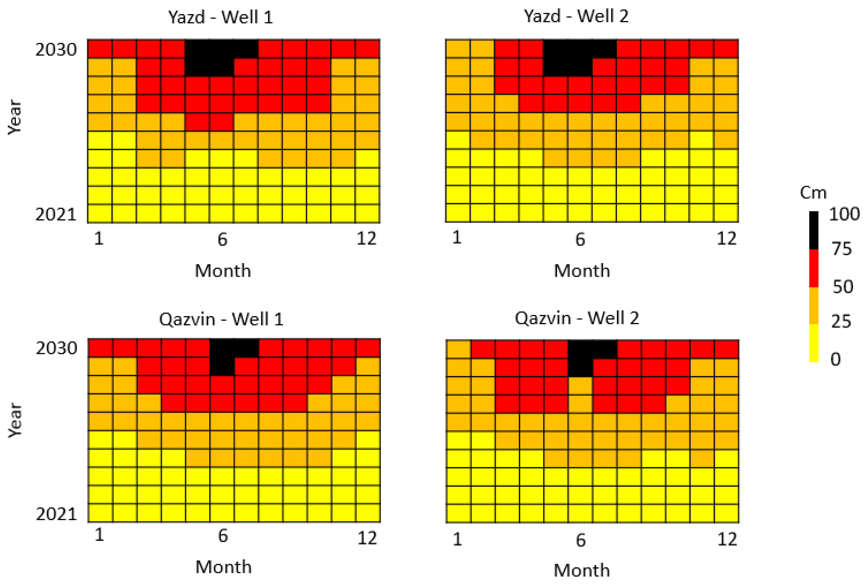
As mentioned in the previous sections, in this study, we tried to take into account all indicators that affect water level changes. They include meteorological changes, agricultural uses and population increases. It was observed that the algorithm has the ability to model water level changes with appropriate accuracy. At this stage, we will predict the changes in groundwater level in the coming years, between 2021 and 2030. The processing process is exactly the same as before. The only difference is the time frame of the prediction of meteorological indicators as stated in Section 4.2. In this case, more accuracy is expected from the final results because the duration of the training period for meteorological data prediction has increased. The groundwater level changes over the period from 2021 to 2030 have been predicted. Figure 14 represents the heatmap plot of the variations in groundwater level depth from 2021 to 2030 compared to the baseline period. The results obtained for the correlation coefficient and its significance test can be seen in Table 9.
Like the previous processing, Figure 14 shows that the most changes occurred in the warmer months of the year. These changes will reach more than 75 cm in 2030. The groundwater level changes for the Yazd region are more than Qazvin. This issue can be attributed to the rapid decrease in precipitation and the increase in temperature in Yazd compared to Qazvin. The most changes have happened in June and July, which is due to more significant changes in temperature and precipitation in these months.
The calculated coefficients in Table 7 show that the correlation between groundwater level changes and meteorological indicators reaches 76%. In 86% of the cases, the relationship between water level changes and meteorological indicators is significant at the significance level of 0.05. As mentioned before, it takes at least one month to establish a meaningful relationship between the variables. For this reason, the p-Value test was rejected in the first months.

5. Summary and Conclusions

This paper focused on two issues: first, providing a specific and reliable algorithm to predict groundwater level changes, and second, investigating the correlation between these changes and meteorological indicator variations. Two regions in Iran with different weather conditions were considered. Using Sentinel-1A acquisitions, the Interferometric Synthetic Aperture Radar (InSAR) technique and advanced integration methods, the exact location of the subsidence in both areas was determined. The meteorological parameters were downscaled and predicted in these areas using the Statistical DownScaling Model (SDSM), meteorological data, synoptic observations and the General Circulation Model (GCM). The groundwater level prediction was conducted using meteorological data, groundwater level observations, Perceptible Water Vapor (PWV) from Global Positioning System (GPS) measurements and the evapotranspiration index based on the Artificial Neural Network (ANN). Predictions were conducted in two different modes. In the first mode, the prediction was made for the current years to validate the proposed algorithm using observations. In the second mode, the prediction was conducted for future time spans. Comparing the prediction with the observations showed that water vapor and evaporation are very important in predicting surface changes. In addition, the mentioned algorithm has a strong ability to model groundwater level changes due to variations in meteorological parameters if additional effects are removed. After making predictions, the relationship between groundwater level changes and meteorological indicators was studied using the Pearson correlation coefficient. The significance test was performed at the significance level of 0.05 using the p-Value test. The results showed that there is a strong relationship between groundwater level and meteorological indicators. The value of the multiple correlation coefficient between groundwater level variations and meteorological data reaches more than 70%. In more than 80% of cases, the relationship between groundwater level changes and meteorological parameters is significant.

Author Contributions

Conceptualization, S.H.-A., Y.A. and A.A.-S.; formal analysis, S.H.-A.; writing—original draft, S.H.-A.; supervision—review and editing, Y.A. and A.A.-S. All authors have read and agreed to the published version of the manuscript.

Funding

This research is based upon research funded by the Iran National Science Foundation (INSF) under project No 4001166.

Data Availability Statement

Data underlying the results presented in this paper are not publicly available.

Acknowledgments

Open access article publication charges have been covered by Delft University of Technology.

Conflicts of Interest

The authors declare no conflict of interest.

References

  1. Lüthi, D.; Floch, M.L.; Bereiter, B.; Blunier, T.; Barnola, J.M.; Siegenthaler, U.; Raynaud, D.; Jouzel, J.; Fischer, H.; Kawamura, K.; et al. High-Resolution Carbon Dioxide Concentration Record 650,000-800,000 Years Before Present. Nature 2008, 453, 379–382. [Google Scholar] [CrossRef] [PubMed] [Green Version]
  2. IPCC. Climate Change 2007: Synthesis Report. Contribution of Working Groups I, II and III to the Fourth Assessment Report of the Intergovernmental Panel on Climate Change; Core Writing Team, Pachauri, R.K., Reisinger, A., Eds.; IPCC: Geneva, Switzerland, 2007; 104p. [Google Scholar]
  3. Horton, E.B. Geographical Distribution of Changes in Maximum and Minimum Temperatures. Atmos. Res. 1995, 37, 102–117. [Google Scholar] [CrossRef]
  4. Rosenzweig, C.; Karoly, D.; Vicarelli, M.; Neofotis, P.; Wu, Q.; Casassa, G.; Menzel, A.; Root, T.L.; Estrella, N.; Seguin, B.; et al. Attributing Physical and Biological Impacts to Anthropogenic Climate Change. Nature 2008, 453, 353–358. [Google Scholar] [CrossRef]
  5. Cohen, S.J. Impacts of CO2-induced Climatic change on water resources in the Great Lakes Basin. Clim. Chang. 1986, 8, 135–153. [Google Scholar] [CrossRef]
  6. Holman, I.P. Impacts climate change on groundwater recharge-uncertainty, shortcomings, and the way forward. Hydrogeology 2006, 14, 637–647. [Google Scholar] [CrossRef] [Green Version]
  7. Jykama, M.I.; Sykes, J.F. The impact of climate change on spatially varying groundwater recharge in the Grand River watershed (Ontario). Hydrology 2007, 338, 237–250. [Google Scholar] [CrossRef]
  8. Ng, G.H.C.; McLaughlin, D.; Entekhabi, D.; Scanlon, B.R. Probabilistic analysis of climate change on groundwater recharge. Water Resour. Res. 2010, 46, 1–18. [Google Scholar] [CrossRef]
  9. Luoma, S.; Okkonen, J. Impacts of Future Climate Change and Baltic Sea Level Rise on Groundwater Recharge. Groundwater Levels, and Surface Leakage in the Hanko Aquifer in Southern Finland. Water 2014, 6, 3671–3700. [Google Scholar] [CrossRef] [Green Version]
  10. Ertürk, A.; Ekdal, A.; Gürel, M.; Karakaya, N.; Guzel, C.; Gönenç, E. Evaluating the impact of climate change on groundwater resources in a small Mediterranean watershed. Scince Total Environ. 2016, 499, 437–447. [Google Scholar] [CrossRef] [PubMed]
  11. House, A.; Acreman, M.; Sorensen, J.; Thompson, J. Hydroecological impacts of climate change modelled for a lowland UK wetland. Geophys. Res. Abstr. 2017, 17, 2015–4671. [Google Scholar]
  12. Burgan, H.I. Comparison of different ANN (FFBP, GRNN, RBF) algorithms and Multiple Linear Regression for daily streamflow prediction in Kocasu River, Turkey. Fresenius Environ. Bull. 2022, 31, 4699–4708. [Google Scholar]
  13. Trabelsi, F.; Bel Hadj Ali, S.; Lee, S. Comparison of Novel Hybrid and Benchmark Machine Learning Algorithms to Predict Groundwater Potentiality: Case of a Drought-Prone Region of Medjerda Basin, Northern Tunisia. Remote Sens. 2023, 15, 152. [Google Scholar] [CrossRef]
  14. Haji-Aghajany, S.; Amerian, Y. Assessment of InSAR tropospheric signal correction methods. J. Appl. Remote Sens. 2020, 14, 044503. [Google Scholar] [CrossRef]
  15. Haji-Aghajany, S.; Amerian, Y. Atmospheric phase screen estimation for land subsidence evaluation by InSAR time series analysis in Kurdistan. Iran J. Atmos. Sol. -Terr. Phys. 2020, 164, 81–88. [Google Scholar] [CrossRef]
  16. Zebker, H.A.; Villasenor, J. Decorrelation in interferometric radar echoes, Geoscience and Remote Sensing. IEEE Trans. 1992, 30, 950–959. [Google Scholar] [CrossRef] [Green Version]
  17. Hanssen, R.F. Radar Interferometry: Data Interpretation and Error Analysis; Kluwer Academic Pub: Dordrecht, The Netherlands, 2001. [Google Scholar]
  18. Haji-Aghajany, S.; Voosoghi, B.; Yazdian, A. Estimation of north Tabriz fault parameters using neural networks and 3D tropospherically corrected surface displacement field. Geomatics. Nat. Hazards Risk 2017, 8, 918–932. [Google Scholar] [CrossRef] [Green Version]
  19. Ferretti, A.; Prati, C.; Rocca, F. Permanent scatterers in SAR interferometry, Geoscience and Remote Sensing. IEEE Trans. 2001, 39, 8–20. [Google Scholar] [CrossRef]
  20. Hooper, A.; Zebker, H.; Segall, P.; Kampes, B. A new method for measuring deformation on volcanoes and other natural terrains using InSAR persistent scatterers. Geophys. Res. Lett. 2004, 31, L23611. [Google Scholar] [CrossRef]
  21. Ferretti, A.; Fumagalli, A.; Novali, F.; Prati, C.; Rocca, F.; Rucci, A. A New Algorithm for Processing Interferometric Data-Stacks: SqueeSAR, Geoscience and Remote Sensing. IEEE Trans. 2011, 49, 3460–3470. [Google Scholar] [CrossRef]
  22. Berardino, P.; Fornaro, G.; Lanari, R.; Sansosti, E. A new algorithm for surface deformation monitoring based on small baseline differential SAR interferograms, Geoscience and Remote Sensing. IEEE Trans. 2002, 40, 2375–2383. [Google Scholar] [CrossRef] [Green Version]
  23. Bekaert, D.P.S.; Hooper, A.; Wright, T.J. A spatially-variable power-law tropospheric correction 1145 technique for InSAR data. J. Geophys. Res. Solid Earth 2015, 120, 1345–1356. [Google Scholar] [CrossRef]
  24. Doin, M.P.; Lasserre, C.; Peltzer, G.; Cavalié, O.; Doubre, C. Corrections of stratified tropospheric delays in SAR interferometry: Validation with global atmospheric models. J. Appl. Geophys. 2009, 69, 35–50. [Google Scholar] [CrossRef]
  25. Li, Z.; Fielding, E.; Cross, P.; Preusker, R. Advanced InSAR atmospheric correction: MERIS/MODIS combination and stacked water vapour models. Int. J. Remote Sens. 2009, 30, 3343–3363. [Google Scholar] [CrossRef]
  26. Yu, C.; Li, Z.; Penna, N.T. Interferometric synthetic aperture radar atmospheric correction using a GPS based iterative tropospheric decomposition model. Remote Sens. Environ. 2018, 204, 109–121. [Google Scholar] [CrossRef]
  27. Haji-Aghajany, S.; Amerian, Y. An investigation of three dimensional ray tracing method efficiency in precise point positioning by tropospheric delay correction. J. Earth Space Phys. 2018, 44, 39–52. [Google Scholar] [CrossRef]
  28. Haji-Aghajany, S.; Voosoghi, B.; Amerian, Y. Estimating the slip rate on the north Tabriz fault (Iran) from InSAR measurements with tropospheric correction using 3D ray tracing technique. Adv. Space Res. 2019, 64, 2199–2208. [Google Scholar] [CrossRef]
  29. Cao, Y.; Jónsson, S.; Li, Z. Advanced InSAR tropospheric corrections from global atmospheric models that incorporate spatial stochastic properties of the troposphere. J. Geophys. Res. Solid Earth 2021, 126, e2020JB020952. [Google Scholar] [CrossRef]
  30. Hobiger, T.; Ichikawa, R.; Koyama, R.; Kondo, T. Fast and accurate ray-tracing algorithms for real-time space geodetic applications using numerical weather models. J. Geophys. Res. 2008, 113, 1–14. [Google Scholar] [CrossRef]
  31. Haji-Aghajany, S.; Amerian, Y. Three dimensional ray tracing technique for tropospheric water vapor tomography using GPS measurements. J. Atmos. Sol. -Terr. Phys. 2017, 164, 81–88. [Google Scholar] [CrossRef]
  32. Haji-Aghajany, S.; Amerian, Y. Hybrid Regularized GPS Tropospheric Sensing Using 3-D Ray Tracing Technique. IEEE Geosci. Remote Sens. Lett. 2018, 15, 1475–1479. [Google Scholar] [CrossRef]
  33. Jolivet, R.; Agram, P.S.; Lin, N.Y.; Simons, M.; Doin, M.P.; Peltzer, G.; Li, Z. Improving InSAR geodesy using global atmospheric models. J. Geophys. Res. Solid Earth 2014, 119, 2324–2341. [Google Scholar] [CrossRef]
  34. Khalili, M.A.; Voosoghi, B.; Guerriero, L.; Haji-Aghajany, S.; Calcaterra, D.; Di Martire, D. Mapping of Mean Deformation Rates Based on APS-Corrected InSAR Data Using Unsupervised Clustering Algorithms. Remote Sens. 2023, 15, 529. [Google Scholar] [CrossRef]
  35. Dubrule, O. Comparing splines and kriging. Comput. Geosci. 1984, 10, 327–338. [Google Scholar] [CrossRef]
  36. Prajapat, D.K.; Choudhary, M. Spatial distribution of precipitation extremes over Rajasthan using CORDEX data. ISH J. Hydraul. Eng. 2021, 27, 289–300. [Google Scholar] [CrossRef]
  37. Rahman Hashmi, M.Z.U.; Shamseldin, A.Y.; Melville, B.W. Comparison of MLP-ANN Scheme and SDSM as Tools for Providing Downscaled Precipitation for Impact Studies at Daily Time Scale. J. Earth Sci. Clim. Chang. 2018, 9, 475. [Google Scholar] [CrossRef]
  38. Haji-Aghajany, S.; Amerian, Y.; Amiri-Simkooei, A. Function-Based Troposphere Tomography Technique for Optimal Downscaling of Precipitation. Remote Sens. 2022, 14, 2548. [Google Scholar] [CrossRef]
  39. Gordon, C.; Cooper, C.; Senior, C.; Banks, H.; Gregory, J.; Johns, T.; Mitchell, J.; Wood, R.A. The simulation of SST, sea ice extents and ocean heat transports in a version of the Hadley Centre coupled model without flux adjustments. J. Clim. Dyn. 2000, 16, 147–168. [Google Scholar] [CrossRef]
  40. Wilby, R.L.; Tomlinson, O.J.; Dawson, C.W. Multi-Site Simulation of Precipitation By Conditional Resampling. Clim. Res. 2003, 23, 183–194. [Google Scholar] [CrossRef]
  41. Banerjee, P.; Prasad, R.K.; Singh, V.S. Forecasting of groundwater level in hard rock region using artificial neural network. Environ. Geol. 2009, 58, 1239–1246. [Google Scholar] [CrossRef]
  42. Chang, J.; Wang, G.; Mao, T. Simulation and prediction of supra permafrost groundwater level variation in response to climate change using a neural network model. J. Hydrol. 2015, 529, 1211–1220. [Google Scholar] [CrossRef]
  43. Levenberg, K.A. A Method for the solution of certain non-linear problems in least squares. Q. Appl. Math. 1944, 2, 164–168. [Google Scholar] [CrossRef] [Green Version]
  44. Marquardt, D.W. An algorithm for least-squares estimation of nonlinear parameters. J. Soc. Ind. Appl. Math. 1963, 11, 431–441. [Google Scholar] [CrossRef]
  45. Dach, R.; Lutz, S.; Walser, P.; Fridez, P. Bernese GNSS Software Version 5.2; User manual, Astronomical Institute, University of Bern, Bern Open Publishing: Bern, Switzerland, 2015; ISBN 978-3-906813-05-9. [Google Scholar] [CrossRef]
  46. Bevis, M.; Businger, S.; Herring, T.A.; Rocken, C.; Anthes, R.A.; Ware, R.H. GPS meteorology: Remote sensing of atmospheric water vapor using the Global Positioning System. J. Geophys. Res. Atmos. 1992, 97, 15787–15801. [Google Scholar] [CrossRef]
  47. Haji-Aghajany, S.; Amerian, Y.; Verhagen, S.; Rohm, W.; Schuh, H. The effect of function-based and voxel-based tropospheric tomography techniques on the GNSS positioning accuracy. J. Geod. 2021, 95, 1–17. [Google Scholar] [CrossRef]
  48. Saastamoinen, J. Atmospheric correction for the troposphere and stratosphere in radio ranging satellites. Use Artif. Satell. Geod. 1972, 15, 247–251. [Google Scholar]
  49. Haji-Aghajany, S.; Amerian, Y.; Verhagen, S. B-spline function-based approach for GPS tropospheric tomography. GPS Solut. 2020, 24, 88. [Google Scholar] [CrossRef]
  50. Allen, R.G.; Pereira, L.S.; Raes, D.; Smith, M. Crop Evapotranspiration. FAO Irrigation and Drainage; Paper No. 56; Food and Agriculture Organization of the United Nations: Rome, Italy, 1998. [Google Scholar]
  51. Thornthwaite, C.W. An approach toward a rational classification of climate. Geogr. Rev. 1948, 38, 55–94. [Google Scholar] [CrossRef]
  52. Zhao, Q.; Sun, T.; Zhang, T.; He, L.; Zhang, Z.; Shen, Z.; Xiong, S. High-Precision Potential Evapotranspiration Model Using GNSS Observation. Remote Sens. 2021, 13, 4848. [Google Scholar] [CrossRef]
  53. Rahman, M.M.; Islam, M.O.; Hasanuzzaman, M. Study of effective rainfall for Irrigated Agriculture in South-Eastern Part of Bangladesh. World J. Agric. Sci. 2008, 4, 453–457. [Google Scholar]
  54. Andrade, C. The P-Value and Statistical Significance: Misunderstandings, Explanations, Challenges, and Alternatives. Indian J. Psychol. Med. 2019, 41, 210–215. [Google Scholar] [CrossRef]
  55. United Nations (2021) World Population Prospects: The 2019 Revision. Volume III: Analytical Report. Available online: https://www.un.org/development/desa/pd/news/world-population-prospects-2019-0 (accessed on 1 January 2023).
  56. Morteza, A.; Mahmood, H.; Mohammadreza, L.; Kamran, D. Estimation of water demand function in agricultural, urban and industrial sectors in Mashhad Plain. Mod. Appl. Sci. 2019, 13, 1–11. [Google Scholar]
  57. Hersbach, H.; Dee, D. ERA5 Reanalysis is in Production; ECMWF Newsletter 147; ECMWF: Reading, UK, 2016. [Google Scholar]
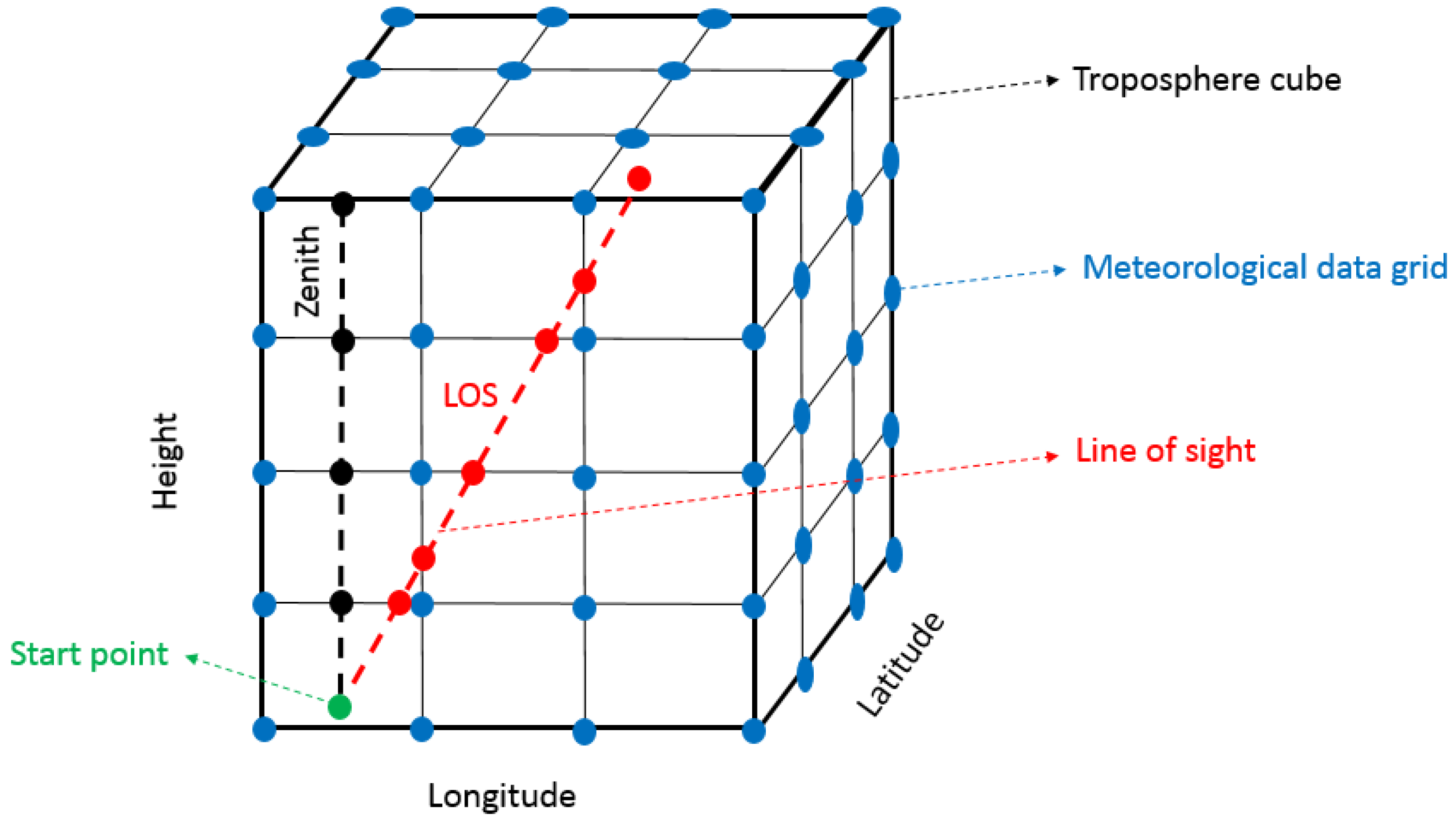
Figure 1. Simple and advanced integration techniques for tropospheric delay computation.
Remotesensing 15 01555 g001
Figure 2. The process of downscaling and production of the scenarios.
Remotesensing 15 01555 g002
Figure 3. Prediction algorithm using ANN.
Remotesensing 15 01555 g003
Figure 4. The geographical location of the study areas. The squares show the position of synoptic and GPS stations and the circles represent the location of groundwater well observations.
Remotesensing 15 01555 g004
Figure 5. Monthly average of precipitation and temperature at the location of the synoptic station from 1979 to 2021, extracted from ERA5 data.
Remotesensing 15 01555 g005aRemotesensing 15 01555 g005b
Figure 6. Processing steps of this study.
Remotesensing 15 01555 g006
Figure 7. Interferograms visualized in the perpendicular and temporal baseline.
Remotesensing 15 01555 g007
Figure 8. A typical example of computed tropospheric delay using the advanced integration technique on 2018-01-04.
Remotesensing 15 01555 g008
Figure 9. Line-of-sight direction displacement velocity maps of two areas. The black star and circles show the location of the reference point and wells, respectively, and the blue square indicates the location of GPS and synoptic stations.
Remotesensing 15 01555 g009
Figure 10. Difference between monthly average of predicted temperature from 2013 to 2020 and base period.
Remotesensing 15 01555 g010
Figure 11. Difference between monthly average of predicted precipitation from 2013 to 2020 and base period.
Remotesensing 15 01555 g011aRemotesensing 15 01555 g011b
Figure 12. Comparison between groundwater level simulation from different input sets and observation in 2020.
Remotesensing 15 01555 g012aRemotesensing 15 01555 g012b
Figure 13. Heatmap plot of difference between monthly average of predicted groundwater level depth from 2013 to 2020 and base period.
Remotesensing 15 01555 g013
Figure 14. Heatmap plot of difference between monthly average of predicted groundwater level depth over 2021 to 2030 and base period.
Remotesensing 15 01555 g014
Table 1. Monthly average of precipitation and temperature from 1979 to 2021.
ParameterAreaJanFebMarAprmayJunJulAugSepOctNovDec
Average precipitation (cm)Qazvin0.500.620.780.750.410.090.050.050.050.330.560.49
Yazd0.280.260.370.300.160.010.010.000.000.050.170.22
Average temperature (k)Qazvin268.8271.9276.9277.0281.8285.9287.2285.9281.0274.2268.1263.8
Yazd282.3285.7289.8289.1294.4298.3298.7296.8292.3285.7280.3276.6
Table 2. Specifications of the radar acquisitions using Sentinel-1A.
AreaMissionProductTrackFlight DirectionBeam ModeTime Span
QazvinSentinel-1AS1A-IW-SLC108DescendingIW2015–2020
YazdSentinel-1AS1A-IW-SLC130AscendingIW2015–2020
Table 3. Statistical properties of groundwater level depth data.
YearAreaMin (m)Max (m)Mean (m)Median (m)
2013
2014
2015
2016
2017
2018
2019
2020
Qazvin
(2 wells)
0.49
0.51
0.58
0.47
0.59
0.57
0.60
0.62
1.86
1.98
2.23
2.39
2.64
2.63
2.71
2.81
1.31
1.29
1.13
1.39
1.28
1.41
1.53
1.61
1.24
1.15
1.11
1.20
1.39
1.47
1.43
1.50
2013
2014
2015
2016
2017
2018
2019
2020
Yazd
(2 wells)
0.50
0.48
0.59
0.63
0.58
0.61
0.67
0.71
2.54
2.64
2.87
2.86
3.12
3.25
3.39
3.31
1.42
1.49
1.69
1.87
1.88
2.01
2.25
2.19
1.31
1.28
1.54
1.63
2.01
2.15
2.11
2.40
Table 4. Statistical measures of observed and downscaled mean monthly temperature during validation period from 2011 to 2012.
AreaVariable (°C)RMSE (°C)NSER2
QazvinTmax0.410.770.85
Tmin0.310.830.87
YazdTmax0.360.790.85
Tmin0.430.840.89
Table 5. Statistical measures of observed and downscaled mean monthly precipitation during validation period from 2011 to 2012.
AreaVariable (mm)RMSE (mm)NSER2
QazvinPrecipitation2.210.750.84
YazdPrecipitation2.020.710.82
Table 6. Different input sets of the ANN. D refers to groundwater level depth.
Set NumberInputs
1Precipitation, Tmin, Tmax, SR, D
2Precipitation, Tmin, Tmax, SR, D, PWV
3Precipitation, Tmin, Tmax, SR, D, ET
4Precipitation, Tmin, Tmax, SR, D, ET, PWV
Table 7. The statistical results of different input sets of ANN.
AreaSet NumberRMSE (m)NSECorrelation
Qazvin10.9890.710.79
Qazvin20.6150.750.82
Qazvin30.3610.810.89
Qazvin40.1890.860.93
Yazd11.0230.700.74
Yazd20.0840.730.81
Yazd30.5980.800.87
Yazd40.2410.840.91
Table 8. Correlation coefficient between changes in groundwater level and meteorological parameters. Green color refers to p-Value smaller than 0.05 and red color shows p-Value greater than 0.05.
MonthJanFebMarAprMayJunJulAugSepOctNovDec
PrecipitationYazd Well 10.390.560.490.540.580.610.680.510.510.680.730.62
Yazd Well 20.400.350.370.480.550.630.690.590.550.630.690.66
Qazvin Well 10.390.460.510.590.500.480.620.510.680.630.750.72
Qazvin Well 20.430.400.490.510.570.510.600.630.710.610.680.66
TemperatureYazd Well 1−0.41−0.37−0.47−0.55−0.59−0.69−0.73−0.75−0.62−0.54−0.48−0.44
Yazd Well 2−0.41−0.42−0.44−0.57−0.65−0.63−0.70−0.67−0.59−0.58−0.68−0.69
Qazvin Well 1−0.36−0.43−0.59−0.55−0.63−0.66−0.62−0.76−0.71−0.66−0.59−0.51
Qazvin Well 2−0.40−0.51−0.46−0.57−0.63−0.59−0.69−0.74−0.71−0.68−0.61−0.59
Table 9. Correlation coefficient between changes in groundwater level and meteorological parameters. Green color refers to p-Value smaller than 0.05 and red shows p-Value greater than 0.05.
MonthJanFebMarAprMayJunJulAugSepOctNovDec
PrecipitationYazd Well 10.310.390.410.610.500.630.690.510.430.650.620.68
Yazd Well 20.310.350.370.470.510.550.500.610.520.580.630.68
Qazvin Well 10.310.330.430.590.680.690.730.760.720.620.690.61
Qazvin Well 20.310.400.510.590.580.630.660.670.710.700.620.53
TemperatureYazd Well 1−0.37−0.42−0.53−0.57−0.61−0.52−0.69−0.61−0.59−0.55−0.51−0.61
Yazd Well 2−0.40−0.33−0.61−0.55−0.51−0.61−0.68−0.53−0.48−0.54−0.49−0.57
Qazvin Well 1−0.37−0.39−0.44−0.51−0.59−0.52−0.46−0.41−0.44−0.58−0.51−0.58
Qazvin Well 2−0.44−0.45−0.51−0.58−0.64−0.67−0.630.51−0.69−0.660.53−0.49
Disclaimer/Publisher’s Note: The statements, opinions and data contained in all publications are solely those of the individual author(s) and contributor(s) and not of MDPI and/or the editor(s). MDPI and/or the editor(s) disclaim responsibility for any injury to people or property resulting from any ideas, methods, instructions or products referred to in the content.