Article

Information Fusion for Spaceborne GNSS-R Sea Surface Height Retrieval Using Modified Residual Multimodal Deep Learning Method

1
School of Geomatics, Liaoning Technical University, Fuxin 123000, China
2
China Academy of Aerospace Science and Innovation, Beijing 100094, China
3
Qian Xuesen Laboratory of Space Technology, China Academy of Space Technology, Beijing 100094, China
4
Shenzhen Institute of Advanced Technology, Chinese Academy of Sciences, Shenzhen 518000, China
*
Author to whom correspondence should be addressed.
These authors contributed equally to this work.
Remote Sens. 2023, 15(6), 1481; https://doi.org/10.3390/rs15061481
Submission received: 17 January 2023 / Revised: 27 February 2023 / Accepted: 3 March 2023 / Published: 7 March 2023
(This article belongs to the Special Issue Precise Point Positioning with GPS, GLONASS, BeiDou, and Galileo II)

Abstract

:
Traditional spaceborne Global Navigation Satellite Systems Reflectometry (GNSS-R) sea surface height (SSH) retrieval methods have the disadvantages of complicated error models, low retrieval accuracy, and difficulty using full DDM information. To compensate for these deficiencies while considering the heterogeneity of the input data, this paper proposes an end-to-end Modified Residual Multimodal Deep Learning (MRMDL) method that can utilize the entire range of DDM information. First, the MRMDL method is constructed based on the modified Residual Net (MResNet) and Multi-Hidden layer neural network (MHL-NN). The MResNet applicable to DDM structures is used to adaptively capture productive features of the full DDM and to convert the two-dimensional DDM data into one-dimensional numerical form. Then, the extracted features and auxiliary parameters are fused as the input data for MHL-NN to retrieve the SSH. Second, the reliability of the model is verified using SSH with tide-corrected DTU Sea Surface Height 18 (DTU18) and spaceborne radar altimeters (Jason3, HY-2C, HY-2B). Compared to the SSH provided by the DTU18 validation model and the spaceborne radar altimeter, the Pearson correlation coefficients (PCC) are 0.98 and 0.97, respectively. However, the CYGNSS satellite is not primarily employed for ocean altimetry, and the mean absolute differences (MAD) are 3.92 m and 4.32 m, respectively. Finally, the retrieval accuracy of the MRMDL method and the HALF retracking approach are compared and analyzed. Finally, this study also implements the HALF retracking algorithm to derive the SSH, and the results are compared with those computed by the MRMDL method. The MRMDL method is more accurate than the HALF retracking approach according to MAD, Root-Mean-Square Error (RMSE), and PCC, with an improvement of 35.21%, 17.25%, and 2.08%, respectively. The MRMDL method will contribute a new theoretical and methodological reference for future GNSS-R altimetry satellites with high spatiotemporal SSH retrieval.

1. Introduction

Satellite altimetry is useful for studying ocean dynamics, environmental factors, and marine gravity fields [1]. The radar altimeters measure the sea surface heights (SSH) along their nadir tracks [2]. However, the spatial resolution is constrained to the period of the satellite; for instance, the period of the exact repeat mission is dozens of days, and the cross-track spacing is larger than 100 km [3]. Different from the radar altimeters which actively transmit signals, the Global Navigation Satellite Systems Reflectometry (GNSS-R) is a bistatic passive microwave radar measurement system [4], that measures the SSH by receiving the signals from GNSS and those signals reflected by the sea surface [5]. Moreover, GNSS-R can simultaneously receive signals from multi-GNSS and provides high spatiotemporal resolution SSH observations [6,7,8].
In 1993, Martin-Neira used GNSS-R to retrieve sea surface height (SSH) for the first time [9]. This technique has been developed and tested on a variety of platforms, including the ground [10], airborne [11,12,13], and spaceborne [14]. The CYGNSS constellation, launched by NASA in December 2016, is the most mature mission to date [15]. CYGNSS consists of eight microsatellites distributed in 510-km orbits, designed to monitor tropical cyclones with high spatiotemporal resolution. To date, a significant number of observations have been obtained. Li et al. processed the raw datasets from the CYGNSS constellation to evaluate the ocean altimetry precision of spaceborne GNSS-R. With 1-s GPS and Galileo group delay measurements, the results demonstrated that the range precision can reach 3.9 and 2.5 m, respectively [16]. Cardellach et al. present the implementation of grazing angle carrier phase sea surface altimetry using the signals transmitted from GPS and Galileo constellations and received by CYGNSS. The results showed that the measurement system achieves decimeter-level SSH retrievals, comparable to spaceborne radar altimeters. The observation conditions, however, are relatively strict: the wind speed must be below 6 m/s and the wave height must be below 1.5 m. Under these conditions, the effective data are only 0.04% of the total observations [17]. Mashburn et al. utilized CYGNSS GNSS-R data to retrieve the SSH in the Indonesian region. In the retrieval process, errors were analyzed and corrected to achieve a retrieval bias of about 6 m [18]. When utilizing spaceborne GNSS-R to retrieve SSH, retracking algorithms, such as HALF, DER, and Z-V models, are typically employed to extract time delay information from the delay waveform (0-Hz Doppler) [19]. However, due to the complex sea surface conditions, these retracking methods may not accurately obtain the time delay of the waveform. Moreover, the received reflected signals by the spaceborne GNSS-R receiver are usually contaminated by background noises because of the high GNSS satellite orbits and low signal transmission power.
Deep learning can compensate for the deficiencies of the above retracking methods because it is an efficient approach to process the enormous data obtained by CYGNSS [20]. Deep learning has been adopted extensively in GNSS-R ocean wind speed retrieval [20,21,22,23,24], soil moisture retrieval [25], and sea ice detection [26] with excellent results. Bu et al. proposed an improved deep learning network framework based on spaceborne GNSS-R data to retrieve global sea surface wind speed; this framework considered auxiliary information including ocean swell, significant wave height (SWH), sea surface rainfall, and wave direction [27]. Yan et al. employed the GALinkNet deep learning method, based on CyGNSS data, to detect inland water bodies; this had better accuracy and effectiveness when compared with other deep networks [28]. Jia et al. employed the XGBoost Machine Learning algorithm to retrieve soil moisture properties from shore-based GNSS-R data [25]. Yan et al. used the CNN algorithm for sea ice detection and density prediction. All achieved remarkable retrieval outcomes [29]. However, deep learning for spaceborne GNSS-R ocean altimetry as still in its preliminary stage. Wang et al. developed a TDS-1 spaceborne GNSS-R SSH retrieval algorithm with delay waveforms, metadata, atmospheric delay, and wind speed as inputs and the corresponding DTU18 SSH as outputs [30]. However, the SSH retrieval method for spaceborne GNSS-R is primarily performed using delayed waveforms.
Different from the previous studies, this study develops the Modified Multimodal Deep Learning (MRMDL) method and employs the full Delay-Doppler Map (DDM) to retrieve SSH measured by CYGNSS. First, the new modified Residual Net model (MResNet) for DDM data structures is employed to adaptively capture productive features of the full DDM and to convert the two-dimensional DDM data into one-dimensional numerical data. Second, the extracted features and auxiliary parameters are fused as the input data for MHL-NN to retrieve the SSH. Third, the performance of the multimodal deep learning method is evaluated by the tide-corrected Danmarks Tekniske Universitet 18 Mean Sea Surface (DTU18MSS) and SSHs from radar altimeters such as Jason3, HY-2C, and HY-2B. Finally, this study also implements the HALF retracking algorithm to derive the SSH, and the results are compared with those computed by the multimodal deep learning method.

2. Data

2.1. CYGNSS Data

The CYGNSS constellation consists of 8 small satellites. Each satellite simultaneously records the reflected signals from four GNSS satellites at 0.5 s intervals, delivering up to 691,200 DDM images every day. Such a massive number of spaceborne measurements provides the foundation for improving the performance of data-driven deep learning algorithms.
In this paper, we use the CYGNSS V3.0 L1 scientific datasets for the experimental data. CYGNSS measurements can be divided into two forms: 11 × 17 two-dimensional image data (DDM) and the corresponding one-dimensional auxiliary parameter data. DDM primarily includes Raw DDM generated by Delay Doppler Mapping Instrument (DDMI) and Bistatic Radar Cross Section (BRCS) DDM after processing. Raw DDM without any processing is a direct measure of scattered signal power and is commonly used for SSH retrieval. BRCS DDM is the primary parameter for sea surface wind speed retrieval. Since BRCS DDM can represent the sea surface wind speed information more significantly, it has a stronger correlation with the sea surface roughness. In this paper, the Raw DDM and the BRCS DDM are used together as the original input data. The auxiliary parameters utilized in this study are presented in Table 1. The first eight elements are CYGNSS L1 level data products, and the remaining four auxiliary parameters are the main error factors for signal path propagation, including ionospheric delay, tropospheric delay, ERA5 U10, and V10 wind speed.
(a) Ionospheric delay: Ionospheric delay will cause range inaccuracies along direct and reflected signal pathways of several meters [19]. The ionospheric delay is estimated using the Global Ionosphere Maps (GIM) of the International GNSS Service (IGS) [31]. The total ionospheric delay can be calculated by the following equation [19]:
δ i o n = ( δ i o n 1 + δ i o n 2 ) δ i o n 3
where δ i o n denotes the total ionospheric delay; δ i o n 1 denotes the ionospheric delay between the GPS transmitting satellite and the specular reflection point (SP); δ i o n 2 denotes the ionospheric delay between the specular reflection point and the CYGNSS satellite; and δ i o n 3 denotes the ionospheric delay between the GPS transmitting satellite and the CYGNSS satellite [32].
(b) Tropospheric delay: The UNB3m model is employed to estimate tropospheric delay [33]. Tropospheric delays are consolidated under 10 km above the ocean surface; therefore, tropospheric correction is only applied to reflected signal paths below the CYGNS spacecraft altitude. The total ionospheric delay can be calculated by the following equation [19]:
δ t r o = ( δ t r o 1 + δ t r o 2 )
where δ t r o denotes the total tropospheric delay; δ t r o 1 denotes the tropospheric delay between the GPS transmitting satellite and the SP; and δ t r o 2 denotes the tropospheric delay between the SP and the CYGNSS satellite;
(c) Wind speed: Sea surface wind speed is measured using ECMWF’s ERA5 reanalysis dataset, which can provide accurate U10 and V10 wind speed data [34]. We matched the CYGNSS dataset to the ERA5 reanalysis dataset with a time window of 1 h and a spatial window of 0.25°.
The heterogeneity of CYGNSS DDM and auxiliary parameter is apparent, as DDM is 2D image data while auxiliary parameter is 1D numerical data. Because of the heterogeneity, straightforward data fusion is not possible. Meanwhile, the low reflected signal power, high noise, and small image size characteristics of DDM make it hard to extract all the effective information using manual feature extraction methods. It will eventually affect the retrieval precision of SSH. A multimodal deep learning method is used to address these issues in this paper. We use MResNet to adaptively extract effective features from the full DDM and transform the 2D image data into 1D numerical data. Then, the extracted features and auxiliary parameters are fused as the input data for MHL-NN to retrieve the SSH.
Liu et al. analyzed the climate state, spatiotemporal distribution, and error characteristics of eight satellite observations of CYGNSS [35]. The results show that the inherent error of CYGNSS wind speed is about 1.8 m/s, which meets the requirements of most operational applications. However, there are inconsistencies in the wind speed measurements between different satellites; the wind speed quality obtained by CY04 satellite is slightly better than other satellites. Therefore, in this paper, measurements from CY04 satellite were selected and analyzed from 1 January 2020 to 31 March 2021.

2.2. DTU 18 Verification Model

To assess the accuracy of spaceborne SSH retrieval, comparison and verification with actual measured SSH are necessary. In this study, we employed a validation model to evaluate the accuracy of the SSH retrieval model due to the lack of real measured SSH data. The DTU18 validation model consists of the DTU18 global mean sea surface (DTU18 MSS) model [36] and the TPXO8 global tide model [37]. The SSH in the validation model can be indicated as [14]:
D T U 18 S S H = D T U 18 + T P X O t i d e
where D T U 18 S S H denotes the SSH of DTU18 verification model and T P X O t i d e denotes the tidal rectification computed by the TPXO8 global tide model.

3. Method

3.1. Construction of the New MRMDL Model

Based on the heterogeneity of inputs data, the architecture of the new MRMDL model suggested in this work is primarily composed of MResNet and MHL-NN. MResNet is utilized to identify effective features from the combination of BRCS DDM and Raw DDM. MHL-NN is employed for SSH retrieval.
(1)
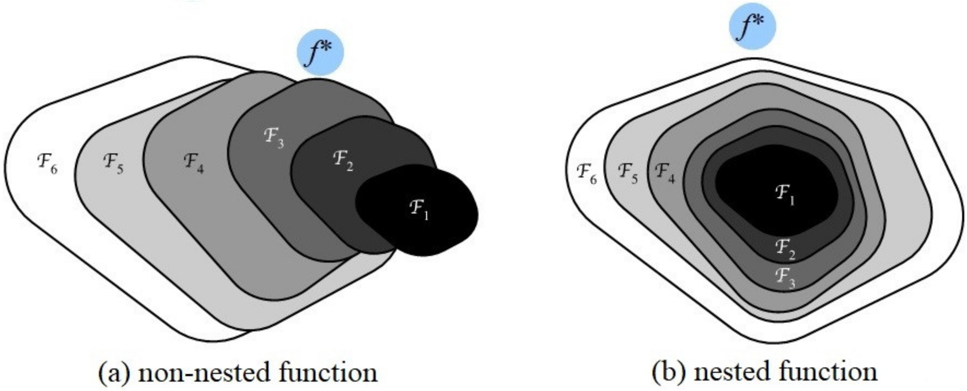
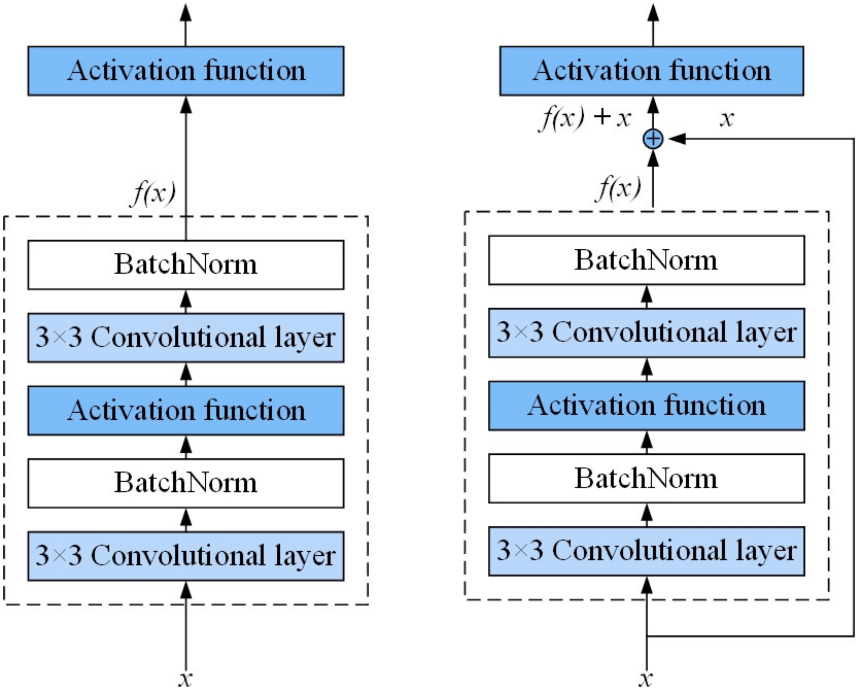
The design of MResNet structure
In this section, the new MResNet model is built to identify the effective features of DDM.
CNN is a neural network designed for image data and composed primarily by convolutional and pooling layers [38,39]. The convolution layer identifies features and eliminates noise by convolving the input data; the pooling layer downsamples the feature map to retain the main features [40]. The depth of the CNN model has a crucial effect on the modelling performance. It is widely assumed that the more layers of convolution and pooling layers used, the more complete the information on image characteristics is collected. Unfortunately, in practical experiments, with the superposition of convolutional and pooling layers, problems such as gradient disappearance (or explosion), overfitting, and degradation problems emerged. The problem of gradient disappearance (or explosion) can be solved by preprocessing the data and using batch normalization layers in the network. Overfitting can be optimized by using Data Augmentation, Regularization, and Dropout. The degradation problem is a phenomenon in which as the depth of the network increases, the network accuracy reaches saturation or even decreases (the training error increases as well). This is primarily because a standard CNN model is a non-nested class of functions [41]. Suppose is the set of a particular class of convolutional neural network architectures; f is our desired objective function. As shown in Figure 1a, for non-nested function classes, functions in more complex function classes (represented by larger areas) are not guaranteed to be closer to the objective function and may be worse (increasing in complexity from A to B). In contrast, for the nested function class in Figure 1b, the simple function class is always contained within the complex function class.
In 2016, He et al. proposed Residual Net (ResNet), that effectively solved the degeneracy problem in deep networks and profoundly influenced the design of subsequent deep neural networks [41]. The foundation of the ResNet is the residual blocks, which suggests that each additional layer should more easily contain the original function as its elements. Figure 2 presents a diagram of the regular convolution block and the residual block. It can be seen that the output of the regular convolution block is f ( x ) , while the output of the residual block not only contains f ( x ) but also adds the original input x . When both the weight and bias parameters of f ( x ) are 0, the function is a constant mapping; the new function class contains the original function class after increasing the number of layers. After adding the residual structure, the CNN becomes a nested function class model, which solves the degradation problem of the CNN network.
Because of the low reflected signal power, high noise, and tiny image size of DDM, the residual structure of ResNet is not suitable for DDM data feature extraction. Therefore, we designed a new modified residual network (MResNet) applicable to the DDM data structure to extract DDM features efficiently. First, the residual block contains two 3 × 3 convolutional layers, with each of these layers followed by a batch normalization layer and a ReLU activation function. Second, by skipping these two convolutional procedures in the cross-layer data path, the input is directly appended preceding the final ReLU activation function. For the outputs of the two convolutional layers to be joined together, they must have the same shape as the inputs. If the number of channels is to be changed, an additional 1 × 1 convolutional is added to convert the input into the required form before the summation operation. In addition, the DDM dimension of L1b is only 17 × 11, and pooling layers would prevent the convolutional layers from maintaining sufficient depth. This would result in the loss of a large amount of valuable information, so the pooling layer is discarded. Finally, because the 17 × 11 DDM data structure is relatively simple, the original number of channels is too large to increase the computation of the model, so the number of channels should be compressed. Table 2 shows the structure of ResNet before and after the modification.
(2)
The structure of the new MRMDL model
A new MRMDL model is schematically structured in Figure 3. It is observed that the new MRMDL model has two input lines. In the first input line, based on the MResNet architecture, features are extracted from the combination of Raw DDM and BRCS DDM by several residual blocks with 3 × 3 convolution kernels. After the feature extraction process, the two-dimensional DDM data are transformed into one-dimensional numerical data. Heterogeneous data are converted to have the same structure. The second input line is used to input auxiliary parameters. The extracted features are fused with the auxiliary parameters in an additional fully connected layer. The fused data are then predicted in the MHL-NN.
Assuming the inputs to the convolutional layer of the new MRMDL model is X1 (i.e., CYGNSS Raw DDM and BRCS DDM) and the inputs to the auxiliary parameters is X2, the model output can be expressed as:
M R M D L S S H = i = 1 L G S σ [ W i N G S ( M R e s N e t ( X 1 ) X 2 ) + b i ]
where M R M D L S S H represents the output of the MRMDL; N G S and L G S denote the optimal number of hidden layers and neurons for each layer determined by the grid search algorithm, respectively; W i and b i denote the i-th hidden layer’s weight and bias, respectively.; M R e s N e t ( X 1 ) denotes the features extracted by the MResNet mode; and σ denotes each hidden layer’s activation function.

3.2. Data Preprocessing

To enhance the convergence of the neural network and improve the generalization ability of the model, the DDM is normalized. The DDM can be normalized by using the following formula [42]:
D D M n o r m a l ( τ , f ) = D D M ( τ , f ) / D D M max
where D D M n o r m a l ( τ , f ) denotes the normalized pixel value; D D M ( τ , f ) denotes the raw pixel value; and D D M max denotes the maximum pixel value in the raw DDM.
The auxiliary parameters also need to be standardized between 0 and 1. The normalization of the auxiliary parameters can be described as follows [42]:
A ( i ) n o r m a l = A ( i ) / A ( i ) max
where A ( i ) denotes the i-th auxiliary parameter; A ( i ) max denotes the maximum value of the i-th auxiliary parameter; and A ( i ) n o r m a l denotes the normalized auxiliary parameter.
Data quality management is crucial to the reasonable use of data during construction of a neural network SSH retrieval model. To guarantee the quality of the dataset, quality control of the CYGNSS dataset is performed according to the following criteria [22].
(a)
Nan samples are all discarded.
(b)
DDM observations should be non-negative.
(c)
All land data should be excluded.
(d)
Data quality control (QC) flags provided by CYGNSS’s L1 level data set: quality_flags = 0, quality_flags_2 = 0.
(e)
The BRCS uncertainty is below 1.
(f)
The range correction gain of DDM is greater than 3
(g)
DDM Signal-to-noise Ratio (SNR) is larger than 5.
(h)
The elevation angle is greater than 60°.
After quality control and data filtering, the daily data were down sampled to alleviate the computational stress and overfitting problems. A total of about 1,071,836 data samples with SSH range between [−100, +80] m were obtained.

3.3. Data Matching

The CYGNSS spaceborne data are continuous time-varying data, while the DTU18 mean sea surface model is a 1′ grid data with latitude and longitude. Therefore, we space-matched the CYGNSS measurements to the DTU18 mean sea surface model (within 0.5′ difference in latitude and longitude). The tide modification is then estimated and applied to the DTU18 MSS. The CYGNSS measurements and the DTU18 validation model comprise the original matchups.
The original matchups are split into training, validation, and test sets. The three datasets did not overlap to confirm the universality of the model throughout time. It can be seen in Figure 4 that the training set is selected for the first 247 days of data in 2020, with about 6.8 × 10⁶ samples, for model training and development. The validation set is selected for the next 92 days of data, with about 1.9 × 10⁶ samples, for the hyperparameter tuning and preliminary model performance evaluation. The test set is selected for a total of 91 days of data from January to March 2021, with about 1.9 × 10⁶ samples. The test data are not involved in model building; the data are only utilized to examine the final accuracy and generalization performance of the model.
In this paper, mean absolute difference (MAD), root mean square error (RMSE), and Pearson Correlation Coefficient (PCC) are adopted to test the reliability of the method [43]. Lesser MAD and RMSE values indicated a favorable fit between the predicted and real values. The closer the PCC is to 1, the better the correlation between the retrieval results and the DTU18 validation model. The corresponding definitions are as follows [43]:
M A D = 1 n i = 1 n | T i A i |
R M S E = 1 n × i = 1 n ( T i A i ) 2
P C C = Cov ( T , A ) σ T σ A
where T denotes the forecast sequence of the model; A denotes the SSH value of the validation model; and n denotes the predicted number of values. Cov ( T , A ) denotes the covariance between the predicted and the validated values; σ T and σ A denote the variance of the estimated and validated values, respectively.

4. Results and Discussion

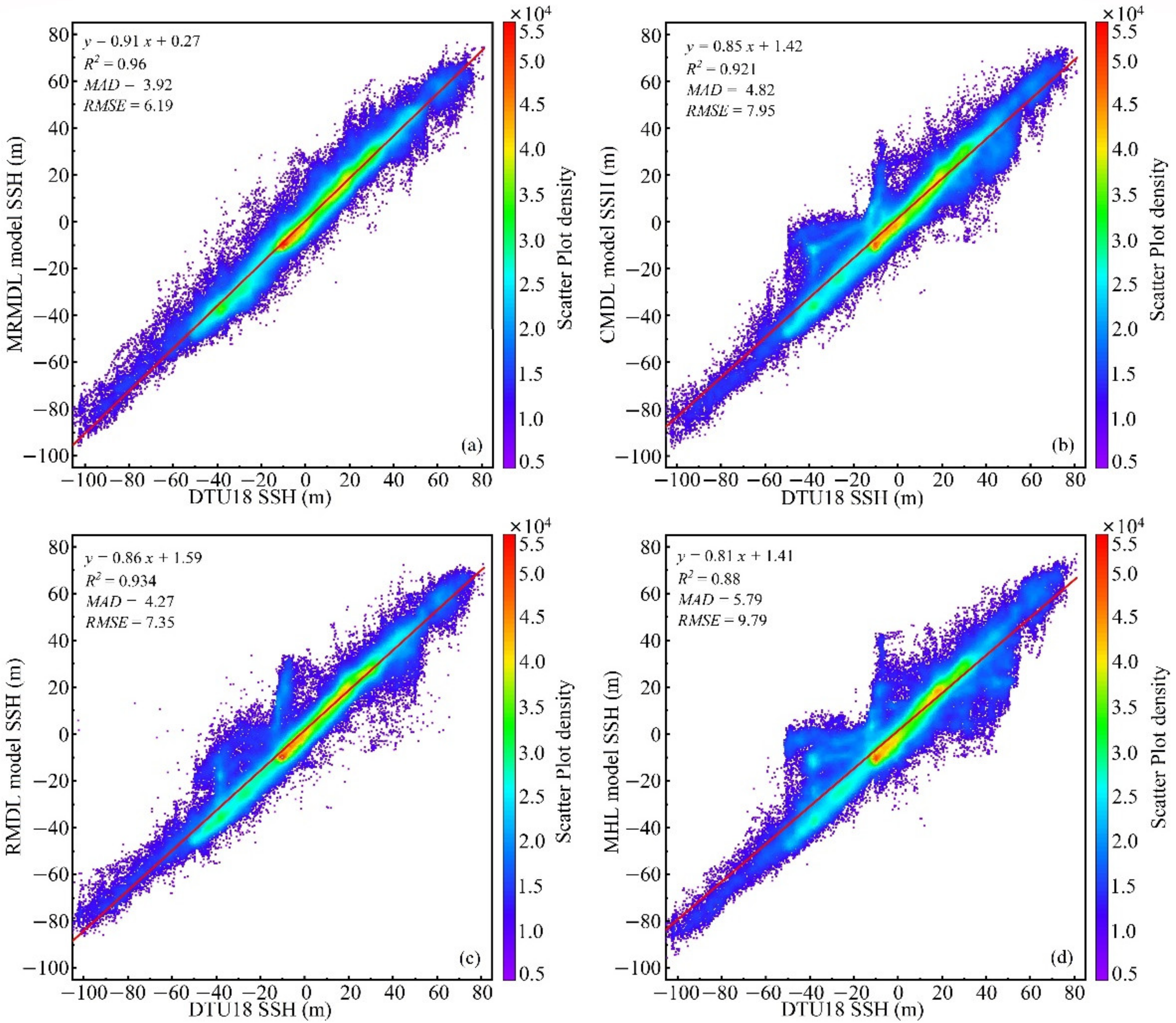
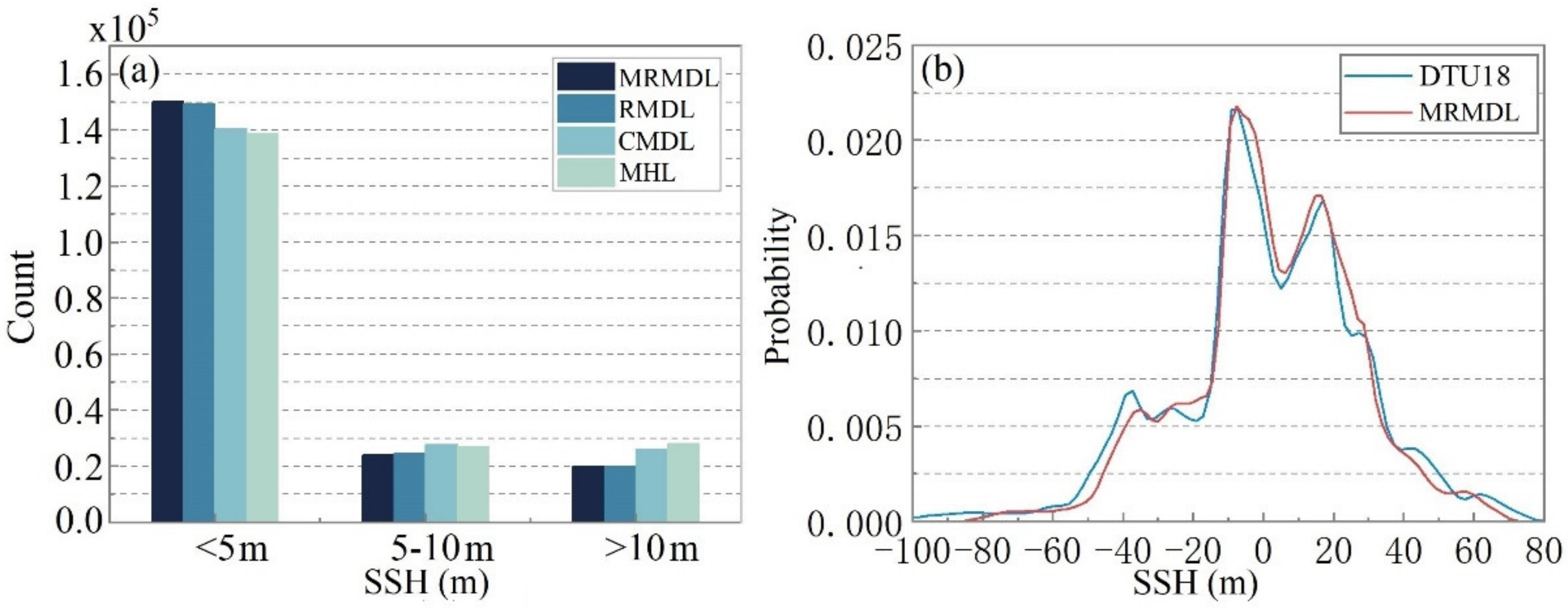
4.1. Validation Using SSH of DTU18 Verification Model

In this section, the retrieval performance of the MHL, CMDL (CNN Multimodal Deep Learning), RMDL (Residual Multimodal Deep Learning), and MRMDL models are compared and analyzed to identify the refinements of the suggested model. Among them, CMDL, RMDL, and MRMDL represent the multimodal deep learning methods comprised of CNN, ResNet, and MResNet feature extraction with MHL, respectively. The models MHL, CMDL, RMDL, and MRMDL are trained on the training set and the hyperparameters of the models are optimized on the validation set. The models’ performances are evaluated by the test set. All models were implemented in PyTorch [24] and trained on a single NVIDIA GeForce RTX2060 GPU.
Table 3 summarizes the number of input and output channels for each layer of all models used in this paper. In the feature extraction stage, RMDL adopts the original structural design of ResNet 50, while CMDL and MRMDL adopt the same channel design solutions. In the SSH retrieval phase, all models used the same MHL design structure with four hidden layers and 200 neurons per layer.
The performance metrics of the four models are statistically illustrated in Table 4. It is evident that the MRMDL model achieves the best retrieval results among the four models. Compared to the DTU18 validation model, the MAD, RMSE, and PCC equal 3.92 m, 6.19 m, and 0.98, respectively. It means that the proposed MRMDL model based on MResNet residual structure can extract the data features of DDM more comprehensively and effectively. Meanwhile, the retrieval results of the CMDL, RMDL, and MRMDL models are better than the MHL model. This demonstrates that the multimodal deep learning models effectively enhance the accuracy of the SSH retrieval when compared to the single model. In addition, the retrieval results from the CMDL, RMDL, and MRMDL models show that the RMDL and MRMDL models can realize a deeper network structure and obtain better retrieval results when compared to the CNN model. Furthermore, the retrieval results from the RMDL and MRMDL models show that the MRMDL model optimized for the DDM data structure can retain more DDM information, resulting in superior retrieval results. Table 3 also gives the average running times of the four models in one epoch. MRMDL, CMDL, and MHL running times are relatively close and much shorter than RMDL.
Figure 5 shows the scatter density plots of the retrieval results for the MRMDL (a), CMDL (b), RMDL (c), and MHL (d) models in relation to the SSH DTU18 validation model. MRMDL retrieval results outperform other models in terms of overall performance and correlated more strongly with the DTU18 validation model, with a PCC of 0.98. However, as the primary purpose of CYGNSS satellites is not ocean altimetry, the satellite receiver is not optimized for SSH retrieval. Its retrieval error is significant, with MAD about 3.92 m and RMSE about 6.19 m. Figure 6a shows the statistical histogram of the error distribution of the four model SSH retrieval results compared to the DTU18 validation model. The statistical results demonstrate that the errors of the four models MRMDL, RMDL, CMDL, and MHL are between −5 and 5 m are 77.33%, 76.92%, 72.34%, and 68.97%, respectively. The retrieval errors between −10 and 10 m are 89.72%, 89.68%, 86.58% and 82.91%, respectively.
Figure 6b depicts the SSH probability density function (PDF) for the MRMDL and DTU18 validation models. It has been demonstrated that the SSH distribution retrieved by MRMDL is generally consistent with the DTU18 validation model. However, in comparison with the DTU18 validation model, the probability of occurrence of SSHs between −60~35 m, 38~54 m, and 60~80 m for MRMDL retrieval is much lower. The probability of occurrence between −25~−15 m and −5~30 m is significantly higher than that of the DTU18 validation model. This is primarily due to the unbalanced distribution of data with various SSHs in the training dataset.
Figure 7a,b presents the global SSH distributions of the DTU18 model and the new MRMDL model, respectively. Figure 7c presents the SSH bias of the new MRMDL method with the DTU18 validation model. Figure 7 demonstrates the overall agreement between the SSH produced by the new MRMDL model and the SSH from the DTU18 validation model. However, the primary use of CYGNSS satellites is not ocean altimetry. The retrieval error is still significant due to the limited DDM time delay resolution, the narrow receiver bandwidth, and the weak peak antenna gain. Figure 7c shows that the SSH bias shows inconsistency in different geographical regions; this is primarily due to the uneven data distribution.

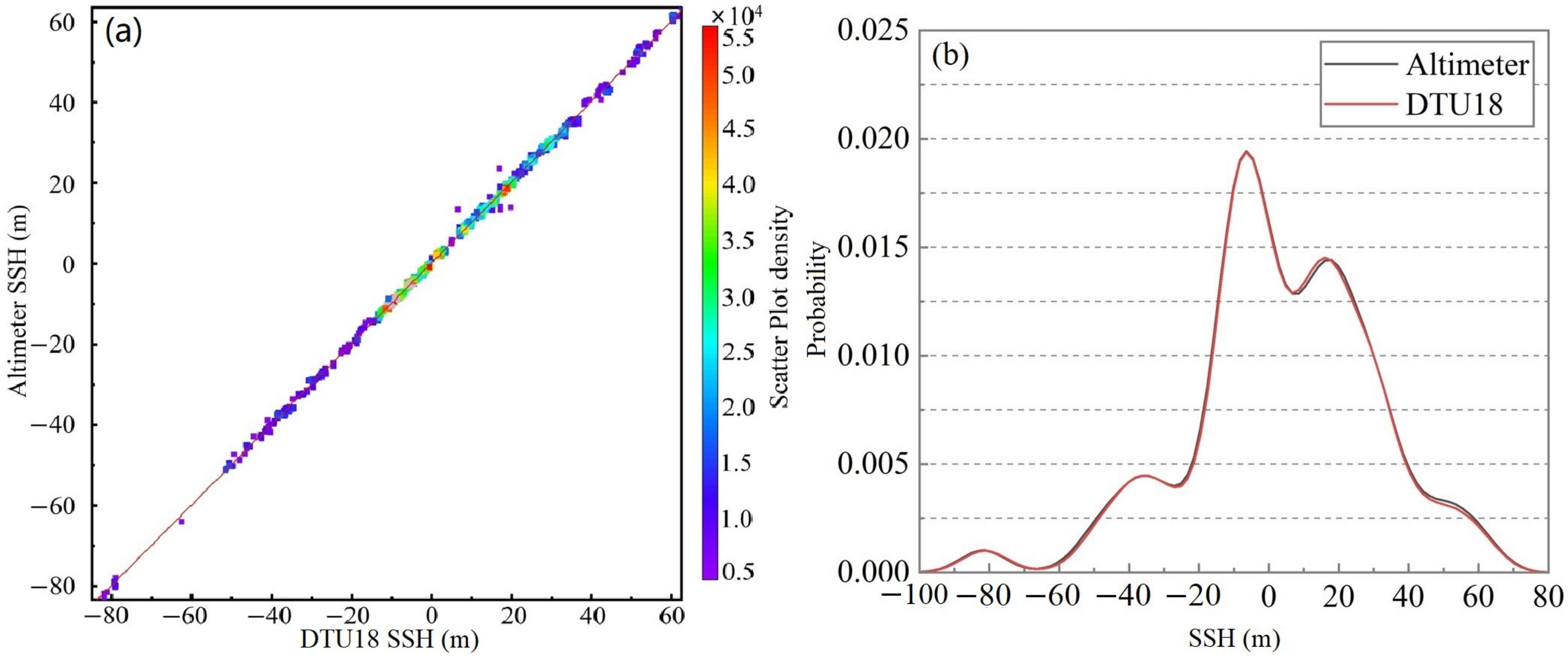
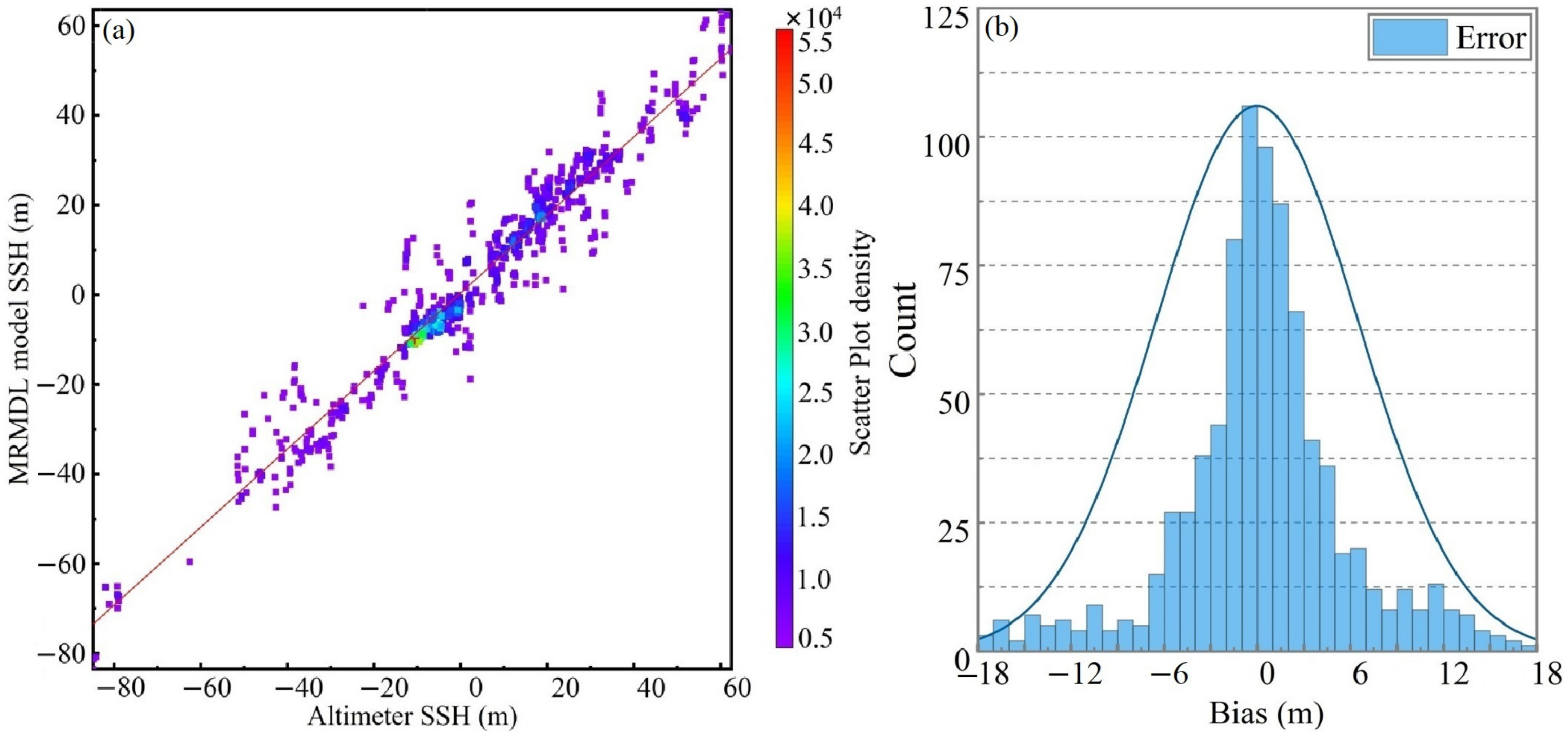
4.2. Validation with SSH of Spaceborne Radar Altimeter

Spaceborne radar altimeters can offer centimeter-level instantaneous SSH measurements [44]. In this section, the data for February and March 2021 are utilized as an example. The SSH retrieval precision of the new MRMDL model was evaluated using the SSH of Jason3, HY-2C, and HY-2B spaceborne radar altimeters [45]. The SSH results of Jason3, HY-2C, and HY-2B altimetry satellites are calculated in this paper using the following equations [46]:
SSH = alt   -   range   -   model _ dry _ tropo _ corr         -   inv _ bar _ corr   -   ocean _ tide _ sol 1   -   solid _ earth _ tide   -   pole _ tide       -   sea _ state _ bias _ ku   -   iono _ corr _ alt _ ku   -   rad _ wet _ tropo _ corr
where alt represents altimeter track height; range represents altimeter measurement distance; model_dry_tropo_corr represents dry troposphere correction; inv_bar_corr represents inverse atmospheric pressure height correction; ocean_tide_soll represents ocean tide correction; solid_earth_tide represents ocean tide correction; pole_tide represents polar tide correction; sea_state_bias_ku represents sea state bias correction; iono_corr_alt_ku represents ionosphere correction; and rad_wet_tropo_corr represents wet troposphere correction.
The SSH of the Jason3, HY-2C, and HY-2B altimetry satellites were spatiotemporally matched (time: 0.5 h, latitude and longitude: 0.25°) with the CYGNSS spaceborne datasets. A total of 865 results were obtained.
Figure 8 compares the SSH of traditional spaceborne radar altimeter and the new MRMDL model. The retrieval results of the new MRMDL can well fit the sea surface height of the radar altimeter. This demonstrates that the retrieval results of the proposed new MRMDL model can well describe the variation of the real SSH. This further validates the effectiveness of the new MRMDL model.
Figure 9a,b present the scatter density and probability distribution plots of SSH for the altimetric satellite and DTU18, respectively. The SSH of the DTU18 validation model has tiny difference and strong correlation with the SSH of the radar altimeter.
Figure 10a,b present the scatter density plots and error distribution histograms of SSH for the radar altimeter and MRMDL models, respectively. The retrieved SSH of the new MRMDL has an extremely strong correlation for the SSH of the radar altimeter, with a PCC of about 0.97. However, because CYGNSS satellites are primarily used for ocean wind speed measurement, they are not optimized for ocean altimetry, due to their own data quality limitations, the MAD and RMSE are 4.32 m and 6.50 m, respectively.

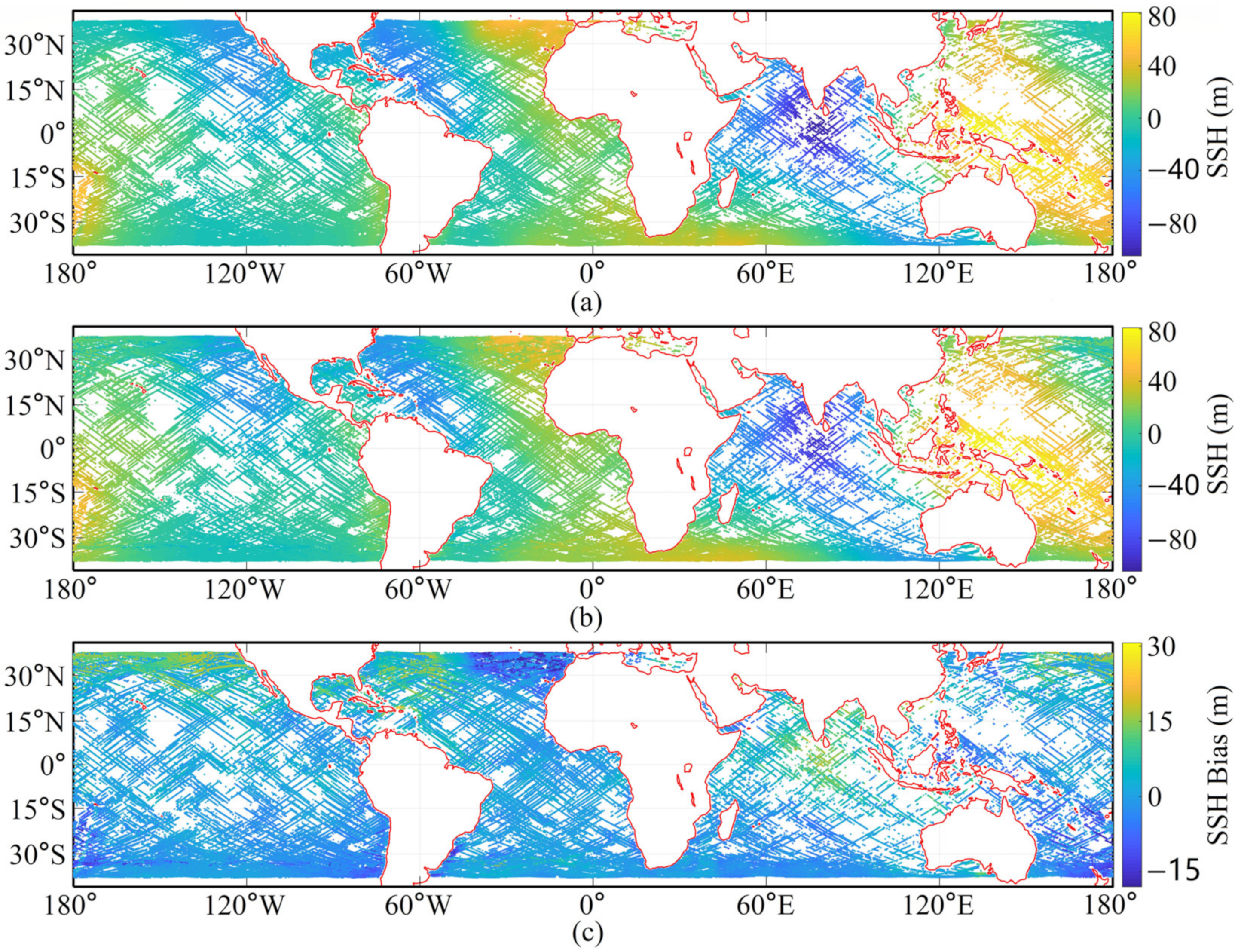
4.3. Application of the New MRMDL Model

To prove the superiority of the MRMDL mode over the conventional spaceborne GNSS-R SSH retrieval method, the retrieval accuracy of both methods was evaluated. The HALF re-tracking method is employed in the traditional SSH retrieval method to calculate the time delay between the reflected signal and the direct signal. The re-tracking point is chosen to be a position on the leading edge of the correlation waveform at 70% of the maximal correlation power. Moreover, the error model in reference [19] corrects for the various errors that are present in the time delay measurements [19]. Figure 11 displays the error statistics of the global SSH as obtained by the MRMDL model and the HALF re-tracking approach. The MRMDL model provides more reliable retrieval outcomes. Approximately 77.3% of the retrieval error for the MRMDL model is between 5 and 5 m, but only 47.89% for the HALF re-tracking approach.
The quantitative precision indicators of the two models are shown in Table 5. The MRMDL outperforms the conventional re-tracking algorithm in precision metrics MAD, RMSE, and PCC. The implementation of MRMDL enhances the accuracy of SSH retrieval. The MAD and RMSE are decreased by 35.21 and 17.25 percent, respectively, and the PCC is enhanced by 2.08 percent. This is primarily because the conventional retracking method compresses the DDM information into a scalar that cannot fully describe the SSH information due to the complex sea surface conditions. The new MRMDL model proposed in this paper can utilize not only the whole DDM information, but also consider more information related to the SSH. Thus, a better retrieval precision can be obtained.

5. Conclusions

The traditional GNSS-R SSH retrieval method has the problems of complicated error model, low retrieval accuracy, and difficulty utilizing DDM information. To compensate for this deficiency, while considering the heterogeneity of the input data, this paper proposes an end-to-end modified deep learning model. The primary conclusions of this paper can be summed up as follows.
(1)
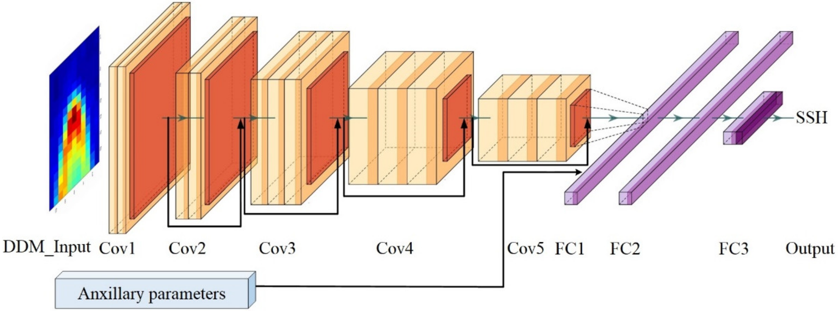
The MRMDL model suggested in this study is primarily composed of MResNet and MHL-NN. First, MResNet is utilized to identify effective features from the combination of BRCS DDM and Raw DDM. Second, the proposed features are fused with the auxiliary parameter data in an additional fully connected layer. Final, MHL-NN is used to retrieve the sea surface height.
(2)
For the DDM reflected signal with low power, high noise, and tiny image size, a residual block applicable to the DDM structure is designed to adaptively identify effective features. The results show that the MResNet can retain more DDM information and produce advantageous retrieval results.
(3)
The reliability of the model was verified using SSH from tide-corrected DTU18 and spaceborne radar altimeters (Jason3, HY-2C, HY-2B). The results illustrate that the presented MRMDL model provides superior retrieval performance. Compared to the DTU18 validated model, the MAD, RMSE, and PCC are 3.92 m, 6.19 m, and 0.98, respectively. Compared to the SSH of the radar altimeter, the MAD, RMSE, and PCC are 4.32 m, 6.50 m, and 0.97, respectively.
(4)
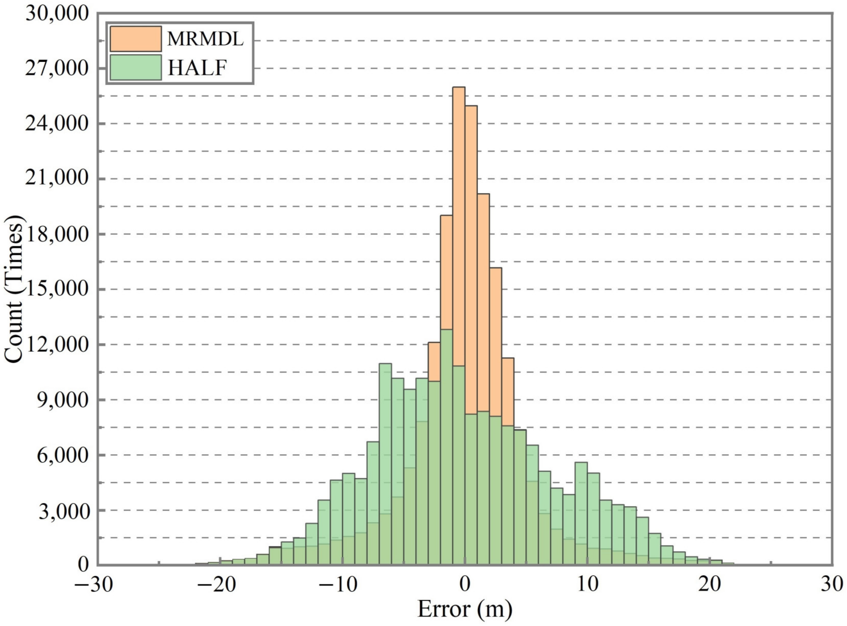
Compared to the traditional HALF re-tracking approach, the SSH retrieval algorithm based on the MRMDL model can significantly improve SSH retrieval precision. The MAD and RMSE are decreased by about 35.21% and 17.25%, respectively; the PCC is enhanced by about 2.08%.
The MRMDL method proposed in this paper will provide new ideas for future DDM-based GNSS-R SSH inversion algorithms. Due to the enormous dataset of GNSS-R, more intelligent and effective data quality control methods need to be applied.

Author Contributions

This study was carried out with the help of all the authors; Q.W.: scientific analysis and manuscript writing. W.Z., F.W. and H.Z.: experiment design, project management, editing. A.X., Y.S. and Y.Z.: review and editing. Q.W., W.Z., F.W. and H.Z. made equal contributions to this paper. All authors have read and agreed to the published version of the manuscript.

Funding

This work was supported in part by the National Natural Science Foundation of China under Grant (42274119), in part by the Liaoning Revitalization Talents Program under Grant (XLYC2002082), in part by National Key Research and Development Plan Key Special Projects of Science and Technology Military Civil Integration (2022YFF1400500), and in part by the Key Project of Science and Technology Commission of the Central Military Commission.

Institutional Review Board Statement

Not applicable.

Informed Consent Statement

Not applicable.

Data Availability Statement

Not applicable.

Conflicts of Interest

The authors declare no conflict of interest.

References

  1. Mashburn, J.; Axelrad, P.; Lowe, S.T.; Larson, K.M. Global ocean altimetry with GNSS reflections from TechDemoSat-1. IEEE Trans. Geosci. Remote Sens. 2018, 56, 4088–4097. [Google Scholar] [CrossRef]
  2. Chen, C.; Zhu, J.; Zhai, W.; Yan, L.; Zhao, Y.; Huang, X.; Yang, W. Absolute calibration of HY-2A and Jason-2 altimeters for sea surface height using GPS buoy in Qinglan, China. J. Oceanol. Limnol. 2019, 37, 1533–1541. [Google Scholar] [CrossRef]
  3. Liu, Z.; Zheng, W.; Wu, F.; Cui, Z.; Kang, G. A Necessary Model to Quantify the Scanning Loss Effect in Spaceborne iGNSS-R Ocean Altimetry. IEEE J. Sel. Top. Appl. Earth Obs. Remote Sens. 2021, 14, 1619–1627. [Google Scholar] [CrossRef]
  4. Wu, F.; Zheng, W.; Liu, Z.; Sun, X. Improving the Specular Point Positioning Accuracy of Ship-borne GNSS-R Observations in China’s Seas based on a new Instantaneous Sea Reflection Surface Model. Front. Earth Sci. 2021, 9, 112–122. [Google Scholar] [CrossRef]
  5. Liu, Z.; Zheng, W.; Wu, F.; Kang, G.; Sun, X.; Wang, Q. Relationship Between Altimetric Quality and Along-Track Spatial Resolution for iGNSS-R Sea Surface Altimetry: Example for the Airborne Experiment. Front. Earth Sci. 2021, 9, 730513. [Google Scholar] [CrossRef]
  6. Clarizia, M.P.; Ruf, C.; Cipollini, P.; Zuffada, C. First spaceborne observation of sea surface height using GPS-reflectometry. Geophys. Res. Lett. 2016, 43, 767–774. [Google Scholar] [CrossRef] [Green Version]
  7. Wu, F.; Zheng, W.; Liu, Z. Quantifying GNSS-R Delay Sea State Bias and Predicting Its Variation Based on Ship-Borne Observations in China’s Seas. IEEE Geosci. Remote Sens. Lett. 2022, 19, 1502705. [Google Scholar] [CrossRef]
  8. Liu, Z.; Zheng, W.; Wu, F.; Kang, G.; Li, Z.; Wang, Q.; Cui, Z. Increasing the Number of Sea Surface Reflected Signals Received by GNSS-Reflectometry Altimetry Satellite Using the Nadir Antenna Observation Capability Optimization Method. Remote Sens. 2019, 11, 2473. [Google Scholar] [CrossRef] [Green Version]
  9. Martin-Neira, M. A passive reflectometry and interferometry system (PARIS): Application to ocean altimetry. ESA J. 1993, 17, 331–355. [Google Scholar]
  10. He, Y.; Gao, F.; Xu, T.; Meng, X.; Wang, N. Coastal altimetry using interferometric phase from GEO satellite in quasi-zenith satellite system. IEEE Geosci. Remote Sens. Lett. 2021, 19, 3002505. [Google Scholar] [CrossRef]
  11. Cardellach, E.; Rius, A.; Martín-Neira, M.; Fabra, F.; Nogués-Correig, O.; Ribó, S.; Kainulainen, J.; Camps, A.; D’Addio, S.D. Consolidating the precision of interferometric GNSS-R ocean altimetry using airborne experimental data. IEEE Trans. Geosci. Remote Sens. 2014, 52, 4992–5004. [Google Scholar] [CrossRef]
  12. Wang, Q.; Zheng, W.; Wu, F.; Xu, A.; Zhu, H.; Liu, Z. A new GNSS-R altimetry algorithm based on machine learning fusion model and feature optimization to improve the precision of sea surface height retrieval. Front. Earth Sci. 2021, 9, 730565. [Google Scholar] [CrossRef]
  13. Sun, X.; Zheng, W.; Wu, F.; Liu, Z. Improving the iGNSS-R Ocean Altimetric Precision Based on the Coherent Integration Time Optimization Model. Remote Sens. 2021, 13, 4715. [Google Scholar] [CrossRef]
  14. Wu, F.; Zheng, W.; Li, Z.; Liu, Z. Improving the positioning accuracy of satellite-borne GNSS-R specular reflection point on sea surface based on the ocean tidal correction positioning method. Remote Sens. 2019, 11, 1626. [Google Scholar] [CrossRef] [Green Version]
  15. Ruf, C.S.; Chew, C.; Lang, T.; Morris, M.G.; Nave, K.; Ridley, A.; Balasubramaniam, R. A New Paradigm in Earth Environmental Monitoring with the CYGNSS Small Satellite Constellation. Sci. Rep. 2018, 8, 8782. [Google Scholar] [CrossRef] [Green Version]
  16. Li, W.; Cardellach, E.; Fabra, F.; Ribó, S.; Rius, A. Assessment of spaceborne GNSS-R ocean altimetry performance using CYGNSS mission raw data. IEEE Trans. Geosci. Remote Sens. 2020, 58, 238–250. [Google Scholar] [CrossRef]
  17. Cardellach, E.; Li, W.; Rius, A.; Semmling, M.; Wickert, J.; Zus, F.; Ruf, C.; Buontempo, C. First Precise Spaceborne Sea Surface Altimetry With GNSS Reflected Signals. IEEE J. Sel. Top. Appl. Earth Obs. Remote Sens. 2020, 13, 102–112. [Google Scholar] [CrossRef]
  18. Mashburn, J.; Axelrad, P.; Zuffada, C.; Loria, E.; O’Brien, A.; Haines, B. Improved GNSS-R ocean surface altimetry with CYGNSS in the seas of indonesia. IEEE Trans. Geosci. Remote Sens. 2020, 58, 6071–6087. [Google Scholar] [CrossRef]
  19. Mashburn, J.R. Analysis of GNSS-R Observations for Altimetry and Characterization of Earth Surfaces. Ph.D. Thesis, University of Colorado, Boulder, CO, USA, 2018. [Google Scholar]
  20. Chu, X.; He, J.; Song, H.; Qi, Y.; Sun, Y.; Bai, W.; Li, W.; Wu, Q. Multimodal deep learning for heterogeneous GNSS-R data fusion and ocean wind speed retrieval. IEEE J. Sel. Top. Appl. Earth Obs. Remote Sens. 2020, 13, 5971–5981. [Google Scholar] [CrossRef]
  21. Liu, Y.; Collett, I.; Morton, Y.J. Application of neural network to GNSS-R wind speed retrieval. IEEE Trans. Geosci. Remote Sens. 2019, 57, 9756–9766. [Google Scholar] [CrossRef]
  22. Li, X.; Yang, D.; Yang, J.; Zheng, G.; Han, G.; Nan, Y.; Li, W. Analysis of coastal wind speed retrieval from CYGNSS mission using artificial neural network. Remote Sens. Environ. 2021, 260, 112454. [Google Scholar] [CrossRef]
  23. Guo, W.; Du, H.; Guo, C.; Southwell, B.J.; Cheong, J.W.; Dempster, A.G. Information fusion for GNSS-R wind speed retrieval using statistically modified convolutional neural network. Remote Sens. Environ. 2022, 272, 112934. [Google Scholar] [CrossRef]
  24. Asgarimehr, M.; Arnold, C.; Weigel, T.; Ruf, C.; Wickert, J. GNSS reflectometry global ocean wind speed using deep learning: Development and assessment of CyGNSSnet. Remote Sens. Environ. 2022, 269, 112801. [Google Scholar] [CrossRef]
  25. Jia, Y.; Jin, S.; Savi, P.; Gao, Y.; Tang, J.; Chen, Y.; Li, W. GNSS-R soil moisture retrieval based on a XGboost machine learning aided method: Performance and validation. Remote Sens. 2019, 11, 1655. [Google Scholar] [CrossRef] [Green Version]
  26. Yan, Q.; Huang, W. Sea ice sensing from GNSS-R data using convolutional neural networks. IEEE Geosci. Remote Sens. Lett. 2018, 15, 1510–1514. [Google Scholar] [CrossRef]
  27. Bu, J.; Yu, K.; Zuo, X.; Ni, J.; Li, Y.; Huang, W. GloWS-Net: A Deep Learning Framework for Retrieving Global Sea Surface Wind Speed Using Spaceborne GNSS-R Data. Remote Sens. 2023, 15, 590. [Google Scholar] [CrossRef]
  28. Yan, Q.; Chen, Y.; Jin, S.; Liu, S.; Jia, Y.; Zhen, Y.; Chen, T.; Huang, W. Inland Water Mapping Based on GA-LinkNet From CyGNSS Data. IEEE Geosci. Remote Sens. Lett. 2023, 20, 1500305. [Google Scholar] [CrossRef]
  29. Yan, S.H.; Zhang, N.; Chen, N.C.; Gong, J.Y. Using reflected signal power from the BeiDou geostationary satellites to estimate soil moisture. Remote Sens. Lett. 2019, 10, 1–10. [Google Scholar] [CrossRef]
  30. Wang, Q.; Zheng, W.; Wu, F.; Zhu, H.; Xu, A.; Shen, Y.; Zhao, Y. Improving the SSH Retrieval Precision of Spaceborne GNSS-R Based on a New Grid Search Multihidden Layer Neural Network Feature Optimization Method. Remote Sens. 2022, 14, 3161. [Google Scholar] [CrossRef]
  31. Hernández-Pajares, M.; Juan, J.M.; Sanz, J.; Orus, R.; Garcia-Rigo, A.; Feltens, J.; Komjathy, A.; Schaer, S.C.; Krankowski, A. The IGS VTEC maps: A reliable source of ionospheric information since 1998. J. Geod. 2008, 83, 263–275. [Google Scholar] [CrossRef]
  32. Yan, Z.; Zheng, W.; Wu, F.; Wang, C.; Zhu, H.; Xu, A. Correction of Atmospheric Delay Error of Airborne and Spaceborne GNSS-R Sea Surface Altimetry. Front. Earth Sci. 2022, 10, 730551. [Google Scholar] [CrossRef]
  33. Leandro, R.; Santos, M.; Langley, R.B. UNB neutral atmosphere models: Development and performance. In Proceedings of the 2006 National Technical Meeting of the Institute of Navigation, Monterey, CA, USA, 18–20 January 2006; Volume 2, pp. 564–573. [Google Scholar]
  34. Wang, S. Inversion of GNSS-R Sea Surface Wind Speed Based on Neural Network Model. Master’s Thesis, National Space Science Center, Chinese Academy of Sciences, Beijing, China, 2020. [Google Scholar]
  35. Liu, S. CYGNSS Sea Surface Reflection Signal Calibration and Verification. MD. Thesis, Nanjing University of Information Science and Technology, Nanjing, China, 2022. (In Chinese). [Google Scholar]
  36. Yuan, J.; Guo, J.; Niu, Y.; Zhu, C.; Li, Z. Mean sea surface model over the sea of Japan determined from multi-satellite altimeter data and tide gauge records. Remote Sens. 2020, 12, 4168. [Google Scholar] [CrossRef]
  37. Egbert, G.D.; Erofeeva, S.Y. Efficient inverse modeling of barotropic ocean tides. J. Atmos. Ocean. Technol. 2002, 19, 183–204. [Google Scholar] [CrossRef]
  38. Jiang, C.; Shen, J.; Chen, S.; Chen, Y.; Liu, D.; Bo, Y. UWB NLOS/LOS Classification Using Deep Learning Method. IEEE Commun. Lett. 2020, 24, 2226–2230. [Google Scholar] [CrossRef]
  39. Hu, X.-D.; Wang, X.-Q.; Meng, F.-J.; Hua, X.; Yan, Y.-J.; Li, Y.-Y.; Huang, J.; Jiang, X.-L. Gabor-CNN for object detection based on small samples. Def. Technol. 2020, 16, 1116–1129. [Google Scholar] [CrossRef]
  40. Yang, H.; Zhang, Y.-S.; Yin, C.-B.; Ding, W.-Z. Ultra-lightweight CNN design based on neural architecture search and knowledge distillation: A novel method to build the automatic recognition model of space target ISAR images. Def. Technol. 2022, 18, 1073–1095. [Google Scholar] [CrossRef]
  41. He, K.; Zhang, X.; Ren, S.; Sun, J. Deep residual learning for image recognition. In Proceedings of the 2016 IEEE Conference on Computer Vision and Pattern Recognition (CVPR), Las Vegas, NV, USA, 12 December 2016; pp. 770–778. [Google Scholar]
  42. Reynolds, J.; Clarizia, M.P.; Santi, E. Wind speed estimation from CYGNSS using artificial neural networks. IEEE J. Sel. Top. Appl. Earth Obs. Remote Sens. 2020, 13, 708–716. [Google Scholar] [CrossRef]
  43. Garrison, J.L. A statistical model and simulator for ocean-reflected GNSS signals. IEEE Trans. Geosci. Remote Sens. 2016, 54, 6007–6019. [Google Scholar] [CrossRef]
  44. Zawadzki, L.; Ablain, M. Accuracy of the mean sea level continuous record with future altimetric missions: Jason-3 vs. Sentinel-3a. Ocean Sci. 2016, 12, 9–18. [Google Scholar] [CrossRef] [Green Version]
  45. Wang, J.; Xu, H.; Yang, L.; Song, Q.; Ma, C. Cross-calibrations of the HY-2B altimeter using Jason-3 satellite during the period of april 2019–september 2020. Front. Earth Sci. 2021, 9, 647583. [Google Scholar] [CrossRef]
  46. Man, E.; Dumont, J.P.; Rosmorduc, V.; Picot, N.; Desai, S.; Bonekamp, H.; Figa, J.; Lillibridge, J.; Scharroo, R. Jason-3 Products Handbook; CNES: Belin, Germany; EUMETSAT: Darmstadt, Germany; NOAA: Washington, DC, USA, 2015. [Google Scholar]
Figure 1. Schematic diagram of non-nested function and nested function; (a) Schematic diagram of non-nested functions; (b) Schematic diagram of the nested functions.
Remotesensing 15 01481 g001
Figure 2. Schematic diagram of conventional convolution block and residual block.
Remotesensing 15 01481 g002
Figure 3. Schematic diagram of the structure of the new MRMDL model.
Remotesensing 15 01481 g003
Figure 4. Daily sample counts in training, validation and test sets.
Remotesensing 15 01481 g004
Figure 5. Scatter density plots of different models; (a) Scatter density plot of MRMDL model; (b) Scatter density plot of CMDL model; (c) Scatter density plot of RMDL model; (d) Scatter density plot of MHL model.
Remotesensing 15 01481 g005
Figure 6. Error distribution histograms and probability density functions of the retrieval results of the four models; (a) Error distribution histogram for retrieval results from the four models; (b) MResNet and DTU18 validation model SSH probability density function.
Remotesensing 15 01481 g006
Figure 7. Global SSH and bias of DTU18 model and the new MRMDL model; (a) SSH of DTU18 model; (b) SSH of the new MRMDL model; (c) SSH bias of the new MRMDL model and the DTU18 model.
Remotesensing 15 01481 g007
Figure 8. Comparison of SSH curves between traditional spaceborne radar altimeter and the new MRMDL model.
Remotesensing 15 01481 g008
Figure 9. Scatter density plot and probability density plot of the radar altimeter with DTU18. (a) Scatter density plot of altimeter satellite and DTU18. (b) Probability density plot of radar altimeter and DTU18.
Remotesensing 15 01481 g009
Figure 10. Scatter density plot and error distribution histogram of the altimeter satellite and MRMDL model. (a) Scatter density plot of the MRMDL model and the altimeter satellite. (b) Error distribution histogram.
Remotesensing 15 01481 g010
Figure 11. Statistics of global SSH errors retrieved by HALF retracking method and MRMDL model.
Remotesensing 15 01481 g011
Table 1. Brief information about auxiliary parameters.
SerialVariable NameBrief DescriptionSerialVariable NameBrief Description
1SNRDDM Signal-to-noise ratio7SP_doppDDM Specular point delay column
2SP_incidenceIncidence angle of specular reflection point8ddm_noise_floorDDM noise floor
3rx_to_sp_rangeCYGNSS to specular point distance9Ionosphereionospheric delay
4tx_to_sp_rangeGPS to specular point distance10Tropospheretropospheric delay
5Peak_delayDDM peak delay row11ERA5 U10ERA5 U10 Wind speed
6Peak_doppDDM peak Doppler column12ERA5 V10ERA5 V10 Wind speed
Table 2. ResNet structure and MResNet network structure.
Layer NameResNetResNet Output SizeMResNet MResNet Output Size
Conv1 7 × 7 , 64 112 × 112 3 × 3 , 16 15 × 9
Conv2 3 × 3 max pool 56 × 56 [ 1 × 1 , 16 3 × 3 , 16 1 × 1 , 16 ] × 3 13 × 7
[ 1 × 1 , 64 3 × 3 , 64 1 × 1 , 256 ] × 3
Conv3 [ 1 × 1 , 128 3 × 3 , 128 1 × 1 , 512 ] × 4 28 × 28 [ 1 × 1 , 8 3 × 3 , 8 1 × 1 , 8 ] × 3 11 × 5
Conv4 [ 1 × 1 , 256 3 × 3 , 256 1 × 1 , 1024 ] × 6 14 × 14 [ 1 × 1 , 4 3 × 3 , 4 1 × 1 , 4 ] × 3 9 × 3
Conv5 [ 1 × 1 , 512 3 × 3 , 512 1 × 1 , 2048 ] × 3 7 × 7 [ 1 × 1 , 4 3 × 3 , 4 1 × 1 , 4 ] × 3 7 × 1
Table 3. The number of input and output channels of each layer of the neural network model.
Layer NameRMDLCMDLMRMDLMHL
Conv1(2, 64)(2, 64)(2, 64)-
Conv2(64, 256)(64, 32)(64, 32)-
Conv3(256, 512)(32, 16)(32, 16)-
Conv4(512, 1024)(16, 8)(16, 8)-
Conv5(1024, 2048)(8, 4)(8, 4)-
FC1200200200200
FC2200200200200
FC3200200200200
FC4200200200200
Table 4. Performance metrics of different model retrieval results.
MHLCMDLRMDLMRMDL
MAD (m)5.094.824.273.92
RMSE (m)8.127.957.356.19
PCC0.940.960.970.98
Running Time (s)30.3433.92530.3154.01
Table 5. Comparison of SSH retrieval performance between MRMDL model and HALF re-tracking method.
MAD (m)RMSE (m)PCC
HALF6.057.480.96
MRMDL3.926.190.98
Improve (%)35.2117.252.08
Disclaimer/Publisher’s Note: The statements, opinions and data contained in all publications are solely those of the individual author(s) and contributor(s) and not of MDPI and/or the editor(s). MDPI and/or the editor(s) disclaim responsibility for any injury to people or property resulting from any ideas, methods, instructions or products referred to in the content.

