DEM Generation from GF-7 Satellite Stereo Imagery Assisted by Space-Borne LiDAR and Its Application to Active Tectonics

Abstract

China’s first optical stereo mapping satellite with a sub-meter resolution, GaoFen-7 (GF-7), launched in November 2019, shows significant potential for providing high-resolution topographic and geomorphic data for quantitative research on active tectonics. However, no studies have evaluated the capability of the GF-7-generated digital elevation model (DEM) for quantitatively studying active tectonics. This study aimed to validate the accuracy of the DEMs extracted from GF-7 stereo imagery, with or without ground control points (GCPs), and evaluated the potential of applying GF-7 DEMs to active tectonics. First, GF-7 stereo images were processed to obtain DEMs with a spatial resolution of 2 m, utilizing three different methods, including block adjustment without GCPs, block adjustment with the aid of Google Earth images and SRTM DEM, and block adjustment with GCPs derived from the Ice, Cloud, and land Elevation Satellite-2 (ICESat-2) data. These three generated DEMs were called GF-7 DEM_Method1, GF-7 DEM_Method2, and GF-7 DEM_Method3, respectively, and were verified by the airborne LiDAR data in the Hasishan section of the Haiyuan fault. Second, the capability of the GF-7 DEMs for identifying active faults, fault scarps, and horizontal offsets was evaluated. Finally, 8 vertical and 13 horizontal offsets were measured based on three different GF-7 DEMs, and airborne LiDAR data were used to verify the measurements’ accuracies. The results indicated that the accuracy of GF-7 DEM_Method1 was the worst and that of GF-7 DEM_Method3 was superior to that of GF-7 DEM_Method2. The GF-7 DEMs could effectively identify the apparent fault scarps and horizontal offsets. The RMSE values of the vertical offsets measured based on GF-7 DEM_Method1, GF-7 DEM_Method2, and GF-7 DEM_Method3 were 0.55 m, 0.55 m, and 0.41 m, respectively. The horizontal offsets yielded RMSE values of 3.98 m, 2.52 m, and 1.37 m, respectively. These findings demonstrated that vertical and horizontal offsets could be accurately measured using the DEMs generated from GF-7 stereo images. Meanwhile, our study indicated that the GCPs derived from ICESat-2 data could be utilized to improve the accuracies of the GF-7 DEM, and the measurements of vertical and horizontal offsets.

1. Introduction

With the rapid development of spatial measurement technology and dating methods, active tectonic research has gradually developed from the early qualitative to the quantitative research stage [1,2]. Quantitative research on active tectonics should acquire some quantitative parameters that represent the active tectonic characteristics, for which the acquisition depends on topographic and geomorphic data with high precision and a high resolution [3,4,5,6].

Various methods have been presented to obtain high-precision digital elevation models (DEMs), including traditional topographic field surveys, synthetic aperture interferometry radar (InSAR), light detection and ranging (LiDAR), unmanned aerial vehicle (UAV) surveys, and high-resolution satellite stereo mapping. Since traditional measurement methods are time-consuming and labor-intensive, it is challenging to obtain large-scale, high-precision topographic data along the entire fault [3]. Although airborne LiDAR can obtain sub-meter high-precision topographic data, it cannot be applied to large areas due to its high acquisition cost [2,7,8]. Recently, the combination of UAV technology and the structure from motion (SfM) photogrammetry method has provided high portability and flexibility, significantly reducing the cost of acquiring high-resolution topographic and geomorphic data [9]. However, applying this method to large areas with a harsh climate and complex terrain is challenging. Although InSAR can obtain topographic data for a large area, the accuracy of its data cannot be guaranteed because the data processing technique is not yet mature [10,11]. The emergence of DEM extraction based on high-resolution satellite stereo imagery provides a new solution for the rapid acquisition of large-scale topographic and geomorphic data in fault zones [6,12,13], significantly reducing the cost and improving the efficiency of acquiring topographic and geomorphic data.

Many previous studies have used commercial high-resolution stereo images such as QuickBird, Pleiades 1A/1B, and WorldView-1/2/3/4 to perform quantitative research on active tectonics [14,15,16,17]. However, these commercial images are expensive and have poor timeliness, restricting their application in the field of active tectonics. China’s first optical stereo mapping satellite with a sub-meter resolution, Gaofen-7 (GF-7), was successfully launched in 2019. The satellite is equipped with a dual-line-array stereo camera comprising a front-view camera and a rear-view camera. It can effectively acquire panchromatic stereo images with a width of 20 km and a resolution of 0.8 m, and multi-spectral images with a resolution of 3.2 m [18]. Although GF-7 exhibits significant potential for providing large-scale high-resolution topographic and geomorphic data, research has yet to explore the potential of applying the GF-7 data to the quantitative study of active tectonics.

Ground control points (GCPs) are necessary to realize accurate DEM generation based on GF-7 stereo images [19,20]. However, acquiring GCPs in the field is often time-consuming and laborious, especially in deserts, woodlands, and areas with complex terrain. Many previous studies have utilized public geographic information data such as Google Earth images and SRTM DEM to improve the accuracy of block adjustments, thereby improving the accuracy of DEMs generated from stereo images [21,22,23]. Recently, with the rapid development of space-borne LiDAR, reliable GCPs have been provided for the block adjustment of satellite stereo images. Existing studies have extracted GCPs using the multi-beam micro-pulse photon-counting LiDAR Ice, Cloud, and land Elevation Satellite-2 (ICESat-2). Although it can effectively improve the accuracy of DEM extraction based on stereo images [24,25], no research has explored the effect of DEM extraction with or without GCPs on the measurement accuracy of active tectonic parameters.

This study aimed to validate the accuracy of the GF-7-extracted DEMs with or without ICESat-2-derived GCPs, and evaluate the potential of applying GF-7 DEMs to active tectonics. In particular, there were three specific objectives: (1) to verify the accuracy of GF-7 DEMs with or without GCPs; (2) to assess the ability of GF-7 DEMs to identify active faults, fault scarps, and horizontal offsets; and (3) to evaluate the potential application of GF-7 DEMs to horizontal and vertical offset measurements with or without GCPs. Ultimately, this study attempted to answer the following questions: (1) Is there any difference between the accuracies of DEMs extracted from GF-7 with and without ICESat-2 derived GCPs? (2) What horizontal and vertical offset levels can be identified on the basis of GF-7 DEMs? (3) Are there any differences in the measurement accuracies of horizontal and vertical offsets with or without the GCPs extracted from ICESat-2 data?

2. Study Site and Materials

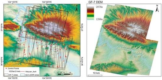
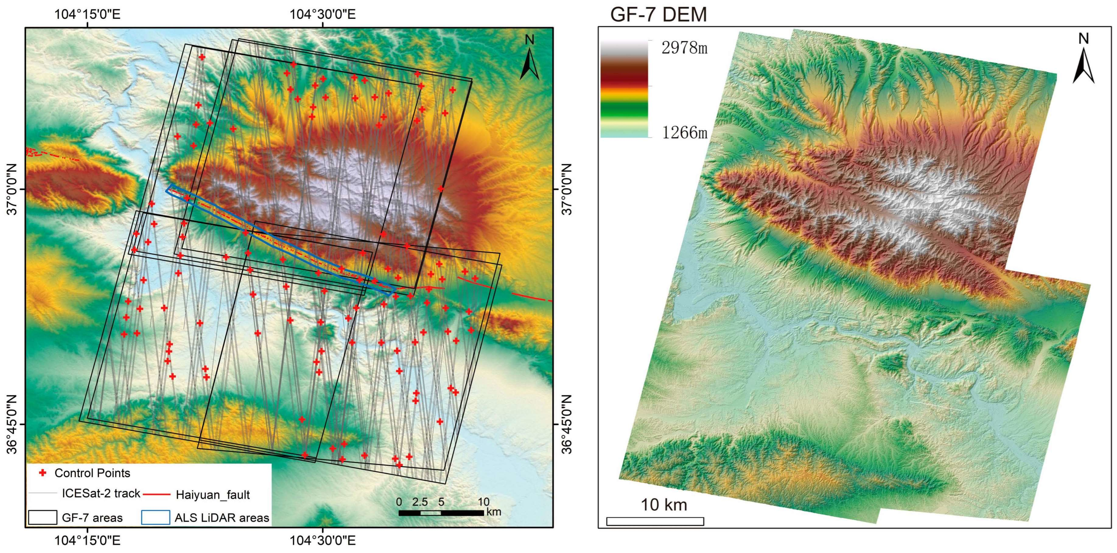
2.1. Study Site

The Haiyuan fault is one of the most critical faults in the northeastern margin of the Tibetan Plateau. It connects with the eastern Liupanshan pediment fault to the east and the Maomaoshan fault to the west (Figure 1a). It is one of the fault zones with the most significant tectonic deformation in the northeastern margin of the Tibetan Plateau [26]. Many large earthquakes have been documented in the history of the Haiyuan fault, such as the M8.5 Haiyuan earthquake in 1920 and the M8–8.3 Gulang earthquake in 1927. The Haiyuan fault is dominated by a left-lateral strike–slip with a small thrust component. Because of their long-term activity, numerous typical strike–slip dislocation landforms have developed along the Haiyuan fault, forming various offset levels. Moreover, the dry climatic environment of the Haiyuan fault makes the landforms well-preserved. In summary, the Haiyuan fault is ideal for quantitative research on active faults [4].

The study area is located in the Hasishan section of the Haiyuan fault (Figure 1b), including various fault scarps, water system dislocations, and trough landforms. The Hasishan section has obvious topographic relief and less vegetation coverage, which is helpful for evaluating the application potential of DEMs extracted from GF-7 data on active tectonics.

2.2. GF-7 Data

The GF-7 is China’s first civil optical stereo mapping satellite with a sub-meter resolution. It was successfully launched in November 2019 with an orbital altitude of about 506 km and a return cycle period of fewer than 60 days. GF-7 aims to generate 1:10,000 stereo mapping products and update large-scale basic geographic information products [27,28]. It can effectively acquire 20 km wide front-view panchromatic stereoscopic images with a 0.8 m resolution, rear-view panchromatic stereoscopic images with a 0.65 m resolution, and multi-spectral images with a 2.6 m resolution. In this study, four GF-7 stereo images from December 2019 to December 2020 with less cloud and snow, a clear texture, and geometric structures were provided by the High-resolution Remote Sensing Data Center, China Earthquake Administration.

Table 1. Details of the GF-7 stereo images used in this study.

Number	Sensor	Product Level	Product ID	Acquisition Time	Cloud Ratio	Coordinate System
1	Dual-line-array camera	LEVEL1A	11181	4 December 2019	5%	WGS 84
2	Dual-line-array camera	LEVEL1A	11182	4 December 2019	5%	WGS 84
3	Dual-line-array camera	LEVEL1A	51458	11 February 2020	5%	WGS 84
4	Dual-line-array camera	LEVEL1A	264266	7 December 2020	1%	WGS 84

lists the specific information of these four GF-7 stereo images.

2.3. ICESat-2/ATLAS Data

ICESat-2 data were utilized to obtain GCPs to improve the accuracy of block adjustments of the GF-7 stereo images. ICESat-2 was launched in 2018 and is equipped with a multi-beam, micro-pulse photon-counting LiDAR system named the Advanced Topographic Laser Altimeter System (ATLAS), which can generate overlapping footprints with a diameter of 12 m spaced at 0.7 m intervals, covering an areas from 88°S to 88°N [29]. ATLAS emits three pairs of beams, each containing strong and weak beams. The cross-track distances between and within the pairs are about 3.3 km and 90 m [30].

ICESat-2 data products are divided into Level 1, Level 2, Level 3A, and Level 3B. The Level-3 A product, ATL08, records the elevation of every 100 m segment. The latest ATL08 data (Version 5) from October 2018 to May 2022 were downloaded through the website https://search.earthdata.nasa.gov/ (accessed on 2 October 2022). In order to select high-precision GCPs, 15 parameters were extracted from the ATL08 data, including the longitude, latitude, elevation, and other parameters (

Table 2. Details of the ATL08 product and the extracted parameters.

Space-Borne LiDAR	ICESat-2/ATLAS
Product	ATL08
Version	Version 5
Vertical datum	WGS 84 ellipsoid
Terrain parameters	h_te_best_fit
Location parameters	latitude, longitude
Other parameters	atlas_beam_type: dummy indicating strong beams or weak beams
	cloud_flag_atm: cloud confidence flag
	dem_h: the elevation of the terrain of the reference DEM
	h_te_skew: the skewness of the heights of the ground photons
	h_te_uncertainty: uncertainty of the mean terrain height for the 100 m segment
	n_ca_photons: the number of canopy photons within the 100 m segment
	n_te_photons: the number of ground photons within the 100 m segment
	n_toc_photons: the number of top of canopy photons within the 100 m segment
	night_flag: dummy indicating the data acquisition time, 0 = day, 1 = night
	segment_landcover: land cover surface type classification, where 60 represents bare, sparse vegetation
	subset_te_flag: quality flag
	terrain_slope: the along-track terrain slope of each 100 m segment

).

2.4. Airborne LiDAR Data

The airborne LiDAR data used in this study were collected in 2011 with a Leica ALS-60 system [3,4]. The swath width of the airborne LiDAR data was 1 km, with an average point density of 4–6 points/m². The triangulated irregular network (TIN) interpolation algorithm was utilized to generate DEM products with a spatial resolution of 1 m based on the cloud points. The coordinate system of the produced DEM was the WGS84 universal transverse Mercator (UTM) projection system. The accuracy of the airborne LiDAR DEM’s horizontal and vertical elevation was 0.3 m and 0.2 m, respectively [3,31]. On the basis of the airborne LiDAR-derived DEM, 20 checkpoints with apparent marks were selected to evaluate the horizontal and vertical accuracies of the DEMs extracted from the GF-7 stereo images (Figure 2a). In addition, 8 positions were selected for measurements of the vertical offset and 13 for measurements of the horizontal offset (Figure 2b).

2.5. Ancillary Data

Google Earth images of the study area with a 1 m resolution were downloaded using Shuijingzhu software, and SRTM DEM data with a 30 m resolution were downloaded from the Google Earth Engine (https://code.earthengine.google.com/ (accessed on 11 September 2022)). The geographic coordinate system of the Google Earth images and SRTM DEM was the World Geodetic System 1984 (WGS84). The elevation datum of the SRTM DEM was the WGS84 ellipsoid.

3. Methods

3.1. Extraction of GCPs from ICESat-2/ATLAS Data

Previous studies have demonstrated that ICESat-2/ATLAS data can be used to extract GCPs. In this study, we extracted a total of 58,419 ATL08 points in the study area as the candidates of the GCPs. However, because of the influence of the atmospheric environment, the targets’ characteristics, the hardware, and other factors, only some ATL08 points had high-accuracy elevation data. Thus, only the reliable ATL08 points were selected as the GCPs. This study utilized the GCP extraction strategy proposed by [25] to obtain high-precision GCPs from the ATL08 data. Previous studies have indicated that the strong beams had better elevation accuracy than weak beams, and the beams collected at nighttime also had better elevation accuracy than those collected during the daytime [32]. Additionally, considering that some ATL08 points are densely distributed, the densely distributed ATL08 points were further filtered to ensure the uniform spatial distribution of the GCPs. Therefore, three more filter criteria were added, in line with the method proposed in [25].

Table 3. The criteria for extracting GCPs from the ATL08 data.

Steps	Filter Criteria
1	night_flag = 1
2	atlas_beam_type = strong
3	h_te_uncertainty < 3.4028235 × 1038
4	|h_te_best_fit−dem_h| < 50
5	terrain_slope < 0.05
6	$\mathrm{n}\_\mathrm{te}\_\mathrm{photons} > 50 \mathrm{and} \frac{\mathrm{n}\_\mathrm{te}\_\mathrm{photons}}{\mathrm{n}\_\mathrm{te}\_\mathrm{photons}+\mathrm{n}\_\mathrm{ca}\_\mathrm{photons}+\mathrm{n}\_\mathrm{toc}\_\mathrm{photons}}>0.5$
7	h_te_uncertainty < 327.6
8	h_te_skew < 6.03
9	Five flags of subset_te_flag greater than −1 with the middle three flags equal to 1
10	cloud_flag_atm <= 2
11	segment_landcover = 60
12	The distances between ATL08 points should be larger than 500 m

shows all the filter criteria for the extraction of GCPs. This study only selected the ATL08 points that met all the filtering criteria as the GCPs.

Figure 3 shows the number of points remaining after each data filtering step. Finally, 114 ATL08 points were selected as the GCPs by the 12 filter criteria (Figure 4).

3.2. Extraction of DEMs from GF-7 Stereo Images

For the GF-7 stereo images, the transformation relationship between the images’ coordinates and the object space coordinates (Equation (1)) was expressed by a rational function model (RFM), which contained multiple rational polynomial coefficients (RPCs). These RPCs are often physically meaningless and inaccurate [33]. Therefore, the block adjustment method was used to add the affine transformation parameters of the image for compensation (Equation (2)) and improve the geometric imaging model of the stereo images and the DEM product’s accuracy [27,34,35].

$$\left\{\begin{array}{l}r=\frac{p_1(X,Y,Z)}{p_2(X,Y,Z)}\\ c=\frac{p_3(X,Y,Z)}{p_4(X,Y,Z)}\end{array}\right.$$

(1)

$$\left\{\begin{array}{l}\Delta c=a_0+a_{1}c+a_{2}r\\ \Delta r=b_0+b_{1}c+b_{2}r\end{array}\right.$$

(2)

where (c, r) are the image coordinates; (X, Y, Z) is the object space coordinates; p₁, p₂, p₃, and p₄ are the RPCs; ($\Delta c$, $\Delta r$) are the compensation values of the image coordinates; and a_i, b_i (i = 0, 1, 2) are the affine transformation coefficients.

Currently, there are three commonly used block adjustment methods:

• Block adjustment without GCPs. This method was essential for selecting some tie points in the GF-7 images and calculating the object space coordinates for each pair of GF-7 stereo pixels, utilizing the space-forward intersection. The final object space coordinate of the tie point was the average coordinate of the tie points between each pair of GF-7 stereo pixels. These tie points were utilized as the virtual GCPs in the block adjustment process.
• Block adjustment with the aid of geographic information system (GIS) data. This method utilized the existing GIS data (such as digital orthophoto maps (DOM) and DEMs) to assist the block adjustment of stereo images. First, a large number of cognominal points were obtained through the automatic registration of the GF-7 satellite images and the existing DOM. Second, the DOM and DEM were used to obtain these cognominal points’ horizontal and elevation coordinates, respectively. Finally, these cognominal points were taken as the control points. In addition to the basic geographic information data (the DOM and DEM), public geographic information data can also be utilized. The most commonly used public geographic information data are Google Earth images and SRTM DEM [21,22,23].
• Block adjustment with GCPs. This method used high-precision GCPs to constrain the elevation values of the forward intersection of the GF-7 stereo images. The most commonly used GCPs can be obtained from space-borne LiDAR data, such as ICESat-1/GLAS and ICESat-2/ATLAS.

Space Data Processor (SDP), a large-scale remote sensing image processing software package, was utilized to perform the block adjustment of the GF-7 satellite stereo images. SDP is a comprehensive, highly automated system for processing remote sensing images independently developed by the Land Satellite Remote Sensing Application Center of the Ministry of Natural Resources of the People’s Republic of China. It can realize the three abovementioned block adjustment methods of GF-7 stereo images. The DEMs obtained by block adjustment without the GCPs, with the aid of 1 m Google Earth maps and 30 m SRTM DEM, and with the GCPs extracted from the ICESat-2 data were named GF-7 DEM_Method1, GF-7 DEM_Method2, and GF-7 DEM_Method3, respectively. The coordinate system of these generated GF-7 DEMs was WGS 84.

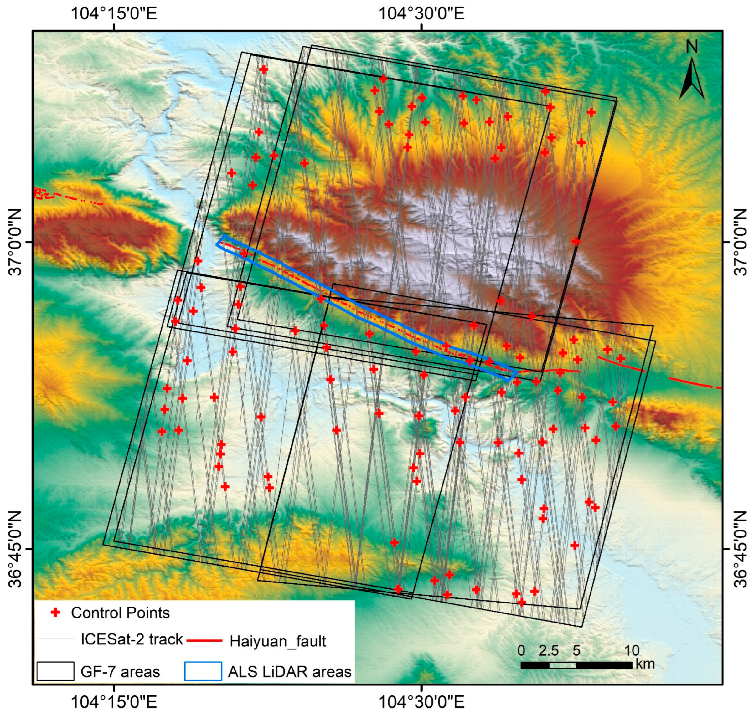
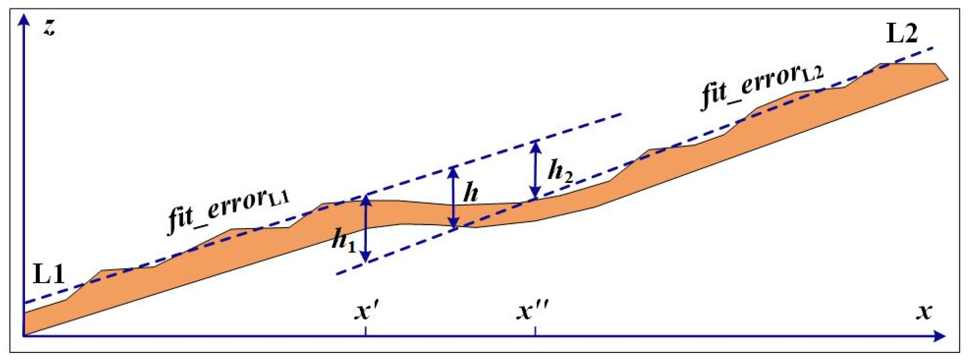
3.3. Measurement of the Horizontal and Vertical Offsets

LaDiCaoz_v2.1 software was adopted to measure the horizontal offsets automatically [14,36]. First, the contour lines were generated based on the DEM to identify the similar geomorphic features of the hanging wall and footwall of the fault. Second, the locations of the fault were identified according to the topographical information and the dislocated geological bodies of the landmark on both sides of the fault were selected for measurement of the horizontal offset (Figure 5a). Third, the characteristics of similar geological bodies on both sides of the fault were compared, and the offsets were automatically matched through horizontal movement, vertical movement, and stretching adjustment (Figure 5c). Finally, the geological body was automatically matched to obtain the optimal horizontal offsets and the dislocation recovery results of the fault (Figure 5b).

In order to extract the height of the fault scarp, global mapper software was utilized to manually extract the survey lines perpendicular to the fault and obtain information on the relative distance and elevation. The vertical offsets and errors were calculated on the basis of the fitting lines of the hanging wall and the footwall of fault according to Equations (3) and (4) [37]. However, undulations in the terrain may cause differences in the elevation between the fitting lines and the DEM. Therefore, the fitting errors of hanging wall and footwall lines were considered (Figure 6).

$$h=\frac{h_1+h_2}{2}$$

(3)

$$\left\{\begin{array}{l}fit\_erro{r}_{\mathit{L}1}=\sqrt{\frac{{\displaystyle \sum _{i=1}^n{(z_i-z_{{\mathit{L}1}_i})}^2}}{n}}(x_i\le x^{\prime })\\ fit\_erro{r}_{\mathit{L}2}=\sqrt{\frac{{\displaystyle \sum _{i=1}^n{(z_i-z_{{\mathit{L}2}_i})}^2}}{n}}(x_i\ge x^{″})\\ dh=\left|\frac{h_1-h_2}{2}\right|+fit\_erro{r}_{L1}+fit\_erro{r}_{L2}\end{array}\right.$$

(4)

where h₁ and h₂ are the fault scarp heights extracted from the fitting line of the hanging wall (L1) and the footwall (L2), respectively; z_i is the DEM’s elevation value at the location x_i; $z_{L{1}_i}$ is the fitted value of the elevation of the hanging wall’s fitting line (L1) at location x_i; and $z_{L{2}_i}$ is the fitted value of the elevation value of the footwall’s fitting line (L2) at location x_i.

3.4. Validation of Accuracy

Airborne LiDAR data were utilized to assess the accuracy of the GF-7 DEMs. Specifically, the 20 checkpoints extracted from the airborne LiDAR data were used to quantitatively evaluate the accuracies of the GF-7 DEMs extracted by the three different block adjustment methods. To further verify the accuracy of the elevation of the GF-7 DEMs, a comparison of the difference between the elevation of the GF-7 DEMs and of the airborne LiDAR data was conducted. As the GF-7 DEMs and airborne LiDAR data were acquired by different methods at different times, they were co-registered to make a reliable comparison. Considering that the accuracy of registration of the LiDAR and GF-7 data based on a point cloud may be higher than that of the interpolated DEMs, we compared the differences in the elevation of the LiDAR and GF-7 point clouds rather than the interpolated DEMs utilizing the software CloudCompare (http://www.danielgm.net/cc/ (accessed on 21 October 2019)). First, the GF-7 DEMs were projected into the UTM system and transformed to point clouds. Second, from the positioning error between GF-7 and airborne LiDAR point clouds, the two point clouds were aligned using the well-known iterative closest point (ICP) algorithm [38]. The GF-7 point clouds were precisely registered with the LiDAR point clouds by iteratively optimizing the rotation matrix and the translation vector. Finally, the differences in the point-to-point elevation between the GF-7 and airborne point clouds were calculated, which only represented the differences in the internal elevation of the two without being affected by their spatial differences [39]. We also evaluated the performance of the GF-7 DEMs by comparing the terrain slopes obtained by the different GF-7 DEMs with terrain slopes calculated on the basis of the airborne LiDAR DEM.

To quantitatively assess the accuracy of the measured horizontal and vertical offsets based on the GF-7 DEMs, the horizontal and vertical offsets measured by the airborne LiDAR-derived DEM were taken as the standard values, and three statistical indicators were included, namely the coefficient of determination (R², Equation (5)), bias (Equation (6)), and the root mean square error (RMSE, Equation (7)).

$${\mathrm{R}}^2=1-\frac{{\displaystyle \sum _{i=1}^n{(y_i-x_i)}^2}}{{\displaystyle \sum _{i=1}^n{(y_i-\overline{y})}^2}}$$

(5)

$$\mathrm{bias}=\frac{{\displaystyle \sum _{i=1}^n(x_i-y_i)}}{n}$$

(6)

$$\mathrm{RMSE}=\sqrt{\frac{{\displaystyle \sum _{i=1}^n{(y_i-x_i)}^2}}{n-1}}$$

(7)

where y_i is the i_th horizontal or vertical offset value extracted from the airborne LiDAR-derived DEM, x_i is the i_th horizontal or vertical offset value extracted from the GF-7 DEM, $\overline{y}$ is the average value of the horizontal or vertical offsets extracted from the airborne LiDAR-derived DEM, and n is the number of horizontal or vertical offsets.

4. Results and Discussion

4.1. Validation of the Accuracy and a Comparison of the GF-7 DEMs

Figure 7 shows the GF-7 DEMs generated by the three different block adjustment methods. The accuracy of the GF-7 DEMs evaluated by 20 checkpoints in the X, Y, and Z directions is shown in

Table 4. Accuracies of the GF-7 DEMs based on checkpoints.

ID	DEMMethod1			DEMMethod2			DEMMethod3
	ΔX (m)	ΔY (m)	ΔZ (m)	ΔX (m)	ΔY (m)	ΔZ (m)	ΔX (m)	ΔY (m)	ΔZ (m)
1	149.77	−201.53	−130.55	4.69	−0.21	5.24	0.50	1.20	1.16
2	148.46	−200.34	−130.39	0.90	0.18	6.04	0.40	2.21	2.55
3	157.04	−201.51	−129.07	3.20	0.63	1.43	0.40	0.73	−2.20
4	158.32	−199.87	−128.46	0.37	−0.38	1.46	0.18	1.63	−2.50
5	163.89	−204.72	−130.49	7.68	−2.97	−2.14	2.42	−3.42	−1.01
6	159.40	−202.56	−127.09	2.14	−3.10	−0.76	−2.03	−0.38	−0.26
7	163.83	−200.53	−124.44	2.26	−0.81	−0.13	0.06	−0.12	−0.75
8	168.24	−198.69	−121.77	3.03	0.42	−0.46	0.45	3.60	−0.53
9	174.50	−201.82	−115.70	2.61	−0.33	2.04	−0.02	0.90	−1.24
10	178.16	−202.59	−111.41	2.25	−3.15	1.57	0.13	0.47	−1.72
11	179.35	−200.34	−108.97	1.16	−2.41	1.76	−0.67	0.20	−0.55
12	182.20	−204.23	−105.27	−0.58	−7.23	1.34	−3.45	−4.60	−1.84
13	188.54	−197.85	−99.99	−0.01	−1.92	1.36	−2.13	0.59	−1.46
14	193.19	−196.84	−92.74	−1.29	−2.35	1.74	−1.07	−0.95	−1.10
15	194.25	−197.83	−92.07	−1.29	−2.53	1.69	−2.35	−0.83	−1.26
16	195.00	−195.72	−91.87	0.05	−0.09	1.59	−1.59	0.88	−1.03
17	194.57	−192.76	−89.07	1.65	−0.99	2.96	0.19	0.23	−0.82
18	199.60	−192.95	−85.52	0.66	0.14	0.39	−0.33	0.90	0.76
19	198.63	−193.20	−86.36	−0.75	−0.04	−0.54	−1.03	0.16	−0.17
20	201.13	−191.41	−82.87	5.06	4.16	1.15	−0.27	0.05	0.49
RMSE	178.24	198.90	110.58	2.80	2.47	2.30	1.38	1.73	1.35

. As shown in Figure 7, the three GF-7 DEMs were not visually significantly different. Table 4 shows that the RMSE values of GF-7 DEM_Method1 were extremely large, namely 178.24 m, 198.90 m, and 110.58 m in the X, Y, and Z directions. The ΔX values gradually increased while the ΔZ values decreased with an increase in the number of checkpoints along the fault. The GF-7 DEM generated by [28] using the block adjustment method without GCPs yielded a plane positioning accuracy of 4.26 m and an elevation accuracy of 8 m. However, the plane positioning and elevation errors of GF-7 DEM_Method1 exceeded 100 m. The reason may be that the GF-7 stereo images used in this paper were mainly collected during the initial operation phase. At this stage, the geometric calibration of GF-7 in orbit was not yet mature, leading to relatively large errors in the horizontal and vertical positioning. The obtained accuracies of GF-7 DEM_Method2 and GF-7 DEM_Method3 were superior to that obtained with DEM_Method1. The RMSE values of GF-7 DEM_Method3 in the X, Y, and Z directions were 1.38 m, 1.73 m, and 1.35 m, respectively. This indicates that the use of GCPs extracted from ICESat-2/ATLAS data significantly improved the accuracy of the generated GF-7 DEMs.

Figure 8 shows the spatial distribution and histogram of the differences in elevation between the GF-7 and LiDAR point clouds. The differences in elevation between the airborne LiDAR and GF-7 DEM_Method1 point clouds mainly ranged from −10 m to 10 m, with a bias of 1.2 m and a standard deviation (STD) of 3.23 m. In contrast to GF-7 DEM_Method1, GF-7 DEM_Method2 and GF-7 DEM_Method3 yielded lower biases of –1.03 m and 0.03 m, and lower STD values of 2.05 m and 1.54 m, respectively. The average difference in the elevation of 0.03 m indicated that GF-7 DEM_Method3 was highly consistent with the airborne LiDAR data, demonstrating that the use of GCPs extracted from ICESat-2/ATLAS data can decrease the differences in elevation between GF-7 DEM and airborne LiDAR data, and improve the accuracy of the elevation of GF-7 DEMs.

To explore the ability of GF-7 DEMs to reproduce the slope, the values of the terrain’s slope were calculated by the DEMs. Figure 9 shows the distribution of the slopes of the terrain calculated by the airborne LiDAR DEM and GF-7 DEMs. The results indicate that the slopes generated by the GF-7 DEMs agreed with those extracted from the airborne LiDAR data in most areas. The differences in the slope between the airborne LiDAR and GF-7 DEMs were also calculated, as shown in Figure 10. The results indicated that GF-7 DEM_Method1 and GF-7 DEM_Method3 were superior to GF-7 DEM_Method2 for reproducing the slope of the terrain.

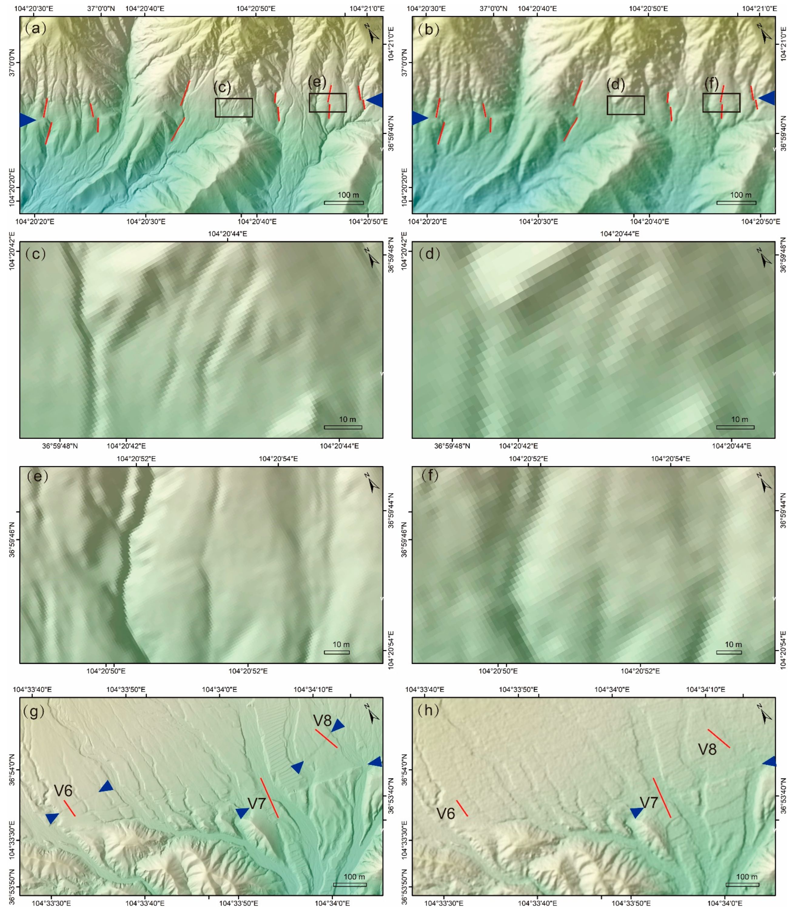
4.2. Observations of the Offset Based on GF-7 DEM

Figure 11 compares the results of active faults, fault scarps, and horizontal fault offsets identified by airborne LiDAR-derived DEM with a 1 m resolution and the GF-7 DEM with a 2 m resolution. As shown in Figure 11, most faults, vertical scarps, and horizontal offsets could be effectively identified by the GF-7 DEM. The GF-7 DEM can be used to identify horizontal offsets larger than 5 m (Figure 11f), while it cannot identify horizontal offsets smaller than 3 m because of the limited resolution (Figure 11d). In addition, the fault scarps, such as V6, with a vertical offset of 0.89 ± 0.04 m, and V8, with a vertical offset of 1.12 ± 0.16 m, could not be effectively identified on the basis of the GF-7 DEM. In short, the GF-7 DEM is suitable for identifying apparent horizontal and vertical offsets over large areas, while it had difficulty identifying fine fault landforms.

4.3. Comparison of the Measurements of the Vertical Offsets

Figure 12 shows the vertical offsets of V1~V8 measured by the airborne LiDAR-derived DEM, GF-7 DEM_Method1, GF-7 DEM_Method2, and GF-7 DEM_Method3. The GF-7 DEMs could reconstruct the fault profile shape with a scarp height larger than 2 m, but significant errors could be observed in the fault profile shape reconstructed by the GF-7 DEMs for small vertical scarps, such as V6 and V8. Figure 13 represents the error scatterplot between the vertical offsets extracted from the airborne LiDAR-derived DEM and the three different GF-7 DEMs. The bias and RMSE values of the vertical offsets measured by GF-7 DEM_Method1 were –0.32 m and 0.55 m. Compared with the significant error in the elevation of GF-7 DEM_Method1 (RMSE = 110.58 m), the accuracy of the vertical offsets measured by GF-7 DEM_Method1 improved significantly, indicating that the absolute elevation error of GF-7 DEM_Method1 was large while the relative elevation error was small. The RMSE and bias values of the vertical offsets measured by GF-7 DEM_Method2 were the same as or smaller than those of GF-7 DEM_Method1. Among these three GF-7 DEMs, the accuracy of the vertical offsets measured by GF-7 DEM_Method3 is the highest, with a bias value of –0.19 m and an RMSE value of 0.41 m. This means that the GCPs extracted from ICESat-2/ATLAS data can slightly improve the accuracy of the measurements of the vertical offsets.

From Figure 13, we can also see most of the measured vertical offsets were generally below the 1:1 line for all three DEMs, suggesting that the vertical offsets may have been underestimated compared with the airborne LiDAR DEM, especially for smaller offset values. The possible reason may be that GF-7 DEMs had a lower resolution (2 m) than the LiDAR DEM (1 m) and cannot reflect the subtle changes in the surface elevation. In other words, the GF-7 DEMs can be regarded as the result obtained after smoothing the LiDAR DTM. In this case, the variation in the elevation of the GF-7 DEMs was smaller than that of the LiDAR DTM, resulting in the vertical offsets being underestimated, especially for smaller offset values.

4.4. Comparison of the Measurements of the Horizontal Offset

Figure 14 shows the horizontal offsets and errors of H1–H13 measured by the airborne LiDAR-derived DEM, GF-7 DEM_Method1, GF-7 DEM_Method2, and GF-7 DEM_Method3. The horizontal offsets extracted by the GF-7 DEMs were compatible with those extracted by the airborne LiDAR-derived DEM.

Table 5. Statistics of the horizontal offsets measured by the airborne LiDAR-derived DEM and the GF-7 DEMs.

DEM	GF-7 DEMMethod1			GF-7 DEMMethod2			GF-7 DEMMethod3
	R2	Bias	RMSE	R2	Bias	RMSE	R2	Bias	RMSE
Statistics	0.99	–1.80 m	3.98 m	1.00	−0.98 m	2.52 m	1.00	–0.81 m	1.37 m

lists the R², bias, and RMSE values of the horizontal offsets extracted by the airborne LiDAR-derived DEM and the GF-7 DEMs. The errors in the horizontal offsets measured by GF-7 DEM_Method1 were the highest, with a bias value of –1.80 m and an RMSE value of 3.98 m. The possible reason is that GF-7 DEM_Method1 had a specific deformation (the horizontal positioning errors in different locations were not constant). Compared with GF-7 DEM_Method1 and GF-7 DEM_Method2, the measured horizontal offsets obtained with GF-7 DEM_Method3 yielded the highest accuracy, with bias and the RMSE values of –0.81 m and 1.37 m, respectively. In other words, the GCPs extracted from ICESat-2/ATLAS data can improve the accuracy of the measurements of horizontal offsets.

5. Conclusions

This study quantitatively evaluated the accuracy of DEMs extracted from GF-7 stereo images with a 2 m resolution with or without GCPs and their potential for application to the quantitative study of active tectonics. The conclusions are as follows: (1) The GF-7 can provide large-scale high-resolution topographical and geomorphological data for quantitatively studying active structures. (2) The GF-7 DEM extracted without GCPs yielded high RMSE values of 178.24 m, 198.90 m, and 110.58 m in the X, Y, and Z directions, respectively. The GCPs extracted from ICESat-2/ATLAS data were used to significantly improve the RMSE values of the GF-7 DEMs in the X, Y, and Z directions to 1.38 m, 1.73 m, and 1.35 m. (3) On the basis of the GF-7 DEMs, the apparent fault scarps and horizontal offsets could be effectively identified, but the fine fault landforms could not be easily identified. (4) Although all three GF-7 DEMs achieved satisfactory accuracy in the measurements of the horizontal and vertical offsets, the GCPs extracted from the ICESat-2/ATLAS data could still improve the accuracy of the measurements of the horizontal and vertical offsets.

In summary, this research indicated, for the first time, the significant potential of China’s first sub-meter stereo mapping satellite, GF-7, for studying active tectonics. However, this study also has some deficiencies, as follows. (1) Only few reliable GCPs were obtained from the ICESat-2 data in the areas with a higher elevation and a rough, steep topography, which may have affected the accuracy of the elevation of the generated GF-7 DEMs. (2) This study only selected the Hasishan section of the Haiyuan fault for research. Therefore, in-depth research should be conducted to explore how to obtain high-precision GCPs from ATL08 data in the area with a rough, steep topography and to analyze the performance of different global DEMs (e.g., the Advanced Land Observing Satellite World 3D (AW3D30) DEM, the Copernicus DEM) in assisting block adjustments of GF-7 data. In addition, we can also select global GF-7 data and sites for measuring the offsets of different levels to improve the reliability of the results.

References

1. Deng, Q.; Chen, L.; Ran, Y. Quantitative Studies and Applications of Active Tectonics. Earth Sci. Front. 2004, 11, 383–392. [Google Scholar] [CrossRef]
2. Ren, Z.; Zielke, O.; Yu, J. Active tectonics in 4D high-resolution. J. Struct. Geol. 2018, 117, 264–271. [Google Scholar] [CrossRef]
3. Liu, J.; Chen, T.; Zhang, P.; Zhang, H.; Zheng, W.; Ren, Z.; Liang, S.; Sheng, C.; Gan, W. Illuminating the Active Haiyuan Fault, China by Airborne Light Detection and Ranging. Chin. Sci. Bull. 2013, 58, 41–45. [Google Scholar] [CrossRef]
4. Chen, T.; Zhang, P.; Liu, J.; Li, C.; Ren, Z.; Hudnut, K. Quantitative study of tectonic geomorphology along Haiyuan fault based on airborne LiDAR. Chin. Sci. Bull. 2014, 59, 2396–2409. [Google Scholar] [CrossRef]
5. Ren, Z.; Zhang, Z.; Chen, T.; Yan, S.; Yin, J.; Zhang, P.; Zheng, W.; Zhang, H.; Li, C. Clustering of offsets on the Haiyuan fault and their relationship to paleoearthquakes. Bulletin 2016, 128, 3–18. [Google Scholar] [CrossRef]
6. Wang, S.; Ren, Z.; Wu, C.; Lei, Q.; Gong, W.; Ou, Q.; Zhang, H.; Ren, G.; Li, C. DEM generation from Worldview-2 stereo imagery and vertical accuracy assessment for its application in active tectonics. Geomorphology 2019, 336, 107–118. [Google Scholar] [CrossRef]
7. Nissen, E.; Maruyama, T.; Arrowsmith, J.R.; Elliott, J.R.; Krishnan, A.K.; Oskin, M.E.; Saripalli, S. Coseismic fault zone deformation revealed with differential lidar: Examples from Japanese M-w similar to 7 intraplate earthquakes. Earth Planet. Sci. Lett. 2014, 405, 244–256. [Google Scholar] [CrossRef]
8. Liu, J.; Ren, Z.; Zhang, H.; Li, C.; Zhang, Z.; Zheng, W.; Li, X.; Liu, C. Slip Rates Along the Laohushan Fault and Spatial Variation in Slip Rate Along the Haiyuan Fault Zone. Tectonics 2022, 41, e2021TC006992. [Google Scholar] [CrossRef]
9. Johnson, K.; Nissen, E.; Saripalli, S.; Arrowsmith, J.R.; McGarey, P.; Scharer, K.; Williams, P.; Blisniuk, K. Rapid mapping of ultrafine fault zone topography with structure from motion. Geosphere 2014, 10, 969–986. [Google Scholar] [CrossRef]
10. Bekaert, D.; Handwerger, A.L.; Agram, P.; Kirschbaum, D.B. InSAR-based detection method for mapping and monitoring slow-moving landslides in remote regions with steep and mountainous terrain: An application to Nepal. Remote Sens. Environ. 2020, 249, 111893. [Google Scholar] [CrossRef]
11. Zhang, Y.; Meng, X.; Dijkstra, T.; Jordan, C.; Chen, G.; Zeng, R.; Novellino, A. Forecasting the magnitude of potential landslides based on InSAR techniques. Remote Sens. Environ. 2020, 241, 111738. [Google Scholar] [CrossRef]
12. Bagnardi, M.; Gonzalez, P.J.; Hooper, A. High-resolution digital elevation model from tri-stereo Pleiades-1 satellite imagery for lava flow volume estimates at Fogo Volcano. Geophys. Res. Lett. 2016, 43, 6267–6275. [Google Scholar] [CrossRef] [Green Version]
13. Shean, D.E.; Alexandrov, O.; Moratto, Z.M.; Smith, B.E.; Joughin, I.R.; Porter, C.; Morin, P. An automated, open-source pipeline for mass production of digital elevation models (DEMs) from very-high-resolution commercial stereo satellite imagery. ISPRS J. Photogramm. Remote Sens. 2016, 116, 101–117. [Google Scholar] [CrossRef] [Green Version]
14. Zhou, Y.; Parsons, B.; Elliott, J.R.; Barisin, I.; Walker, R.T. Assessing the ability of Pleiades stereo imagery to determine height changes in earthquakes: A case study for the El Mayor-Cucapah epicentral area. J. Geophys. Res. Solid Earth 2015, 120, 8793–8808. [Google Scholar] [CrossRef] [Green Version]
15. Martha, T.R.; Govindharaj, K.B.; Kumar, K.V. Damage and geological assessment of the 18 September 2011 M-w 6.9 earthquake in Sikkim, India using very high resolution satellite data. Geosci. Front. 2015, 6, 793–805. [Google Scholar] [CrossRef] [Green Version]
16. Ou, Q.; Kulikova, G.; Yu, J.; Elliott, A.; Parsons, B.; Walker, R. Magnitude of the 1920 Haiyuan Earthquake Reestimated Using Seismological and Geomorphological Methods. J. Geophys. Res. Solid Earth 2020, 125, e2019JB019244. [Google Scholar] [CrossRef]
17. Bi, H.; Zheng, W.; Lei, Q.; Zeng, J.; Zhang, P.; Chen, G. Surface Slip Distribution Along the West Helanshan Fault, Northern China, and Its Implications for Fault Behavior. J. Geophys. Res. Solid Earth 2020, 125, e2020JB019983. [Google Scholar] [CrossRef]
18. Liu, C.; Cui, X.; Guo, L.; Wu, L.; Tang, X.; Liu, S.; Yuan, D.; Wang, X. Satellite Laser Altimetry Data-Supported High-Accuracy Mapping of GF-7 Stereo Images. Remote Sens. 2022, 14, 5868. [Google Scholar] [CrossRef]
19. Chen, J.; Tang, X.; Xue, Y.; Li, G.; Zhou, X.; Hu, L.; Zhang, S. Registration and Combined Adjustment for the Laser Altimetry Data and High-Resolution Optical Stereo Images of the GF-7 Satellite. Remote Sens. 2022, 14, 1666. [Google Scholar] [CrossRef]
20. Sun, Y.; Nie, S.; Li, G.; Huang, X.; Liu, Z.; Wang, C.; Xi, X.; Yu, J. Evaluation of the performance of GaoFen-7 laser altimeter data for ground elevation retrieval over vegetated areas. Remote Sens Lett. 2022, 13, 991–1001. [Google Scholar] [CrossRef]
21. Pan, X.; Jiang, T.; Yu, A.; Zhang, Y.; Yu, L. Block Adjustment of High-Resolution Satellite Images with Google Earth. J. Geomat. Sci. Technol. 2017, 34, 622–627. [Google Scholar]
22. Mumtaz, R.; Palmer, P.L.; Waqar, M.M. Georeferencing of UK DMC stereo-images without ground control points by exploiting geometric distortions. Int. J. Remote Sens. 2014, 35, 2136–2169. [Google Scholar] [CrossRef]
23. Zhou, P.; Tang, X.; Wang, Z.; Cao, N.; Wang, X. SRTM-assisted block adjustment for stereo pushbroom imagery. Photogramm. Rec. 2018, 33, 49–65. [Google Scholar] [CrossRef]
24. Ye, J.; Qiang, Y.; Zhang, R.; Liu, X.; Deng, Y.; Zhang, J. High-Precision Digital Surface Model Extraction from Satellite Stereo Images Fused with ICESat-2 Data. Remote Sens. 2022, 14, 142. [Google Scholar] [CrossRef]
25. Shang, D.; Zhang, Y.; Dai, C.; Ma, Q.; Wang, Z. Extraction Strategy for ICESat-2 Elevation Control Points Based on ATL08 Product. IEEE Trans. Geosci. Remote Sens. 2022, 60, 5705012. [Google Scholar] [CrossRef]
26. Zhang, P.; Peter, M.; Burchfiel, B.C.; Royden, L.; Wang, Y.; Deng, Q.; Song, F.; Zhang, W.; Jiao, D. Bounds on the Holocene Slip Rate of the Haiyuan Fault, North-Central China. Quat. Res. 1988, 30, 151–164. [Google Scholar] [CrossRef]
27. Xie, J.; Huang, G.; Liu, R.; Zhao, C.; Dai, J.; Jin, T.; Mo, F.; Zhen, Y.; Xi, S.; Tang, H.; et al. Design and Data Processing of China’s First Spaceborne Laser Altimeter System for Earth Observation: GaoFen-7. IEEE J. Sel. Top. Appl. Earth Obs. Remote Sens. 2020, 13, 1034–1044. [Google Scholar] [CrossRef]
28. Tang, X.; Liu, C.; Zhang, H.; Wang, X.; Li, G.; Mo, F.; Li, F. GF⁃7 Satellite Stereo Images Block Adjustment Assisted with Laser Altimetry Data. Geomat. Inf. Sci. Wuhan Univ. 2021, 46, 1423–1430. [Google Scholar] [CrossRef]
29. Markus, T.; Neumann, T.; Martino, A.; Abdalati, W.; Brunt, K.; Csatho, B.; Farrell, S.; Fricker, H.; Gardner, A.; Harding, D.; et al. The ice, cloud, and land elevation satellite-2 (ICESat-2): Science requirements, concept, and implementation. Remote Sens. Environ. 2017, 190, 260–273. [Google Scholar] [CrossRef]
30. Neumann, T.A.; Martino, A.J.; Markus, T.; Bae, S.; Bock, M.R.; Brenner, A.C.; Brunt, K.M.; Cavanaugh, J.; Fernandes, S.T.; Hancock, D.W.; et al. The ice, cloud, and land elevation Satellite-2 Mission: A global geolocated photon product derived from the advanced topographic laser altimeter system. Remote Sens. Environ. 2019, 233, 111325. [Google Scholar] [CrossRef]
31. Bi, H.; Zheng, W.; Ren, Z.; Zeng, J.; Yu, J. Using an unmanned aerial vehicle for topography mapping of the fault zone based on structure from motion photogrammetry. Int. J. Remote Sens. 2017, 38, 2495–2510. [Google Scholar] [CrossRef]
32. Liu, A.; Cheng, X.; Chen, Z. Performance evaluation of GEDI and ICESat-2 laser altimeter data for terrain and canopy height retrievals. Remote Sens. Environ. 2021, 264, 112571. [Google Scholar] [CrossRef]
33. Grodecki, J.; Dial, G. Block Adjustment of High⁃Resolution Satellite Images Described by Rational Functions. Photogramm. Eng. Remote Sens. 2003, 69, 59–68. [Google Scholar] [CrossRef]
34. Li, G.; Tang, X.; Gao, X.; Wang, H.; Wang, Y. ZY-3 Block adjustment supported by glas laser altimetry data. Photogramm. Rec. 2016, 31, 88–107. [Google Scholar] [CrossRef]
35. Yang, B.; Wang, M.; Xu, W.; Li, D.; Gong, J.; Pi, Y. Large-scale block adjustment without use of ground control points based on the compensation of geometric calibration for ZY-3 images. ISPRS J. Photogramm. Remote Sens. 2017, 134, 1–14. [Google Scholar] [CrossRef]
36. Zielke, O.; Arrowsmith, J.R.; Ludwig, L.G.; Akciz, S.O. Slip in the 1857 and earlier large earthquakes along the Carrizo Plain, San Andreas Fault. Science 2010, 327, 1119–1122. [Google Scholar] [CrossRef] [Green Version]
37. Ai, M.; Bi, H.; Zheng, W.; Yin, J.; Yuan, D.; Ren, Z.; Chen, G.; Liu, J. Using unmanned aerial vehicle photogrammetry technology to obtain quantitative parameters of active tectonics. Seismol. Geol. 2018, 40, 1276–1293. [Google Scholar] [CrossRef]
38. Rusinkiewicz, S.; Levoy, M. Efficient variants of the ICP algorithm. In Proceedings of the 3rd International Conference on 3-D Digital Imaging and Modeling, Quebec City, QC, Canada, 28 May–1 June 2001. [Google Scholar] [CrossRef] [Green Version]
39. Lague, D.; Brodu, N.; Leroux, J. Accurate 3D comparison of complex topography with terrestrial laser scanner: Application to the Rangitikei canyon (N-Z). ISPRS J. Photogramm. Remote Sens. 2013, 82, 10–26. [Google Scholar] [CrossRef] [Green Version]
Figure 1. (a) Tectonic map of the area around the Haiyuan fault. (b) The Hasishan section of the Haiyuan fault and the coverage areas of the GF-7 stereo images.
Remotesensing 15 01480 g001
Figure 2. The distribution of (a) the checkpoints and (b) the positions for measurement of the vertical and horizontal offset.
Remotesensing 15 01480 g002
Figure 3. The number of ATL08 points remaining after each data filtering step.
Remotesensing 15 01480 g003
Figure 4. The location and distribution of the GCPs extracted from the ICESat-2/ATLAS data.
Remotesensing 15 01480 g004
Figure 5. Measurement of the horizontal offsets using LaDiCaoz_v2.1 software. (a) The faults (light blue), fault-parallel profile lines (red and blue), and the longitudinal tracking line (yellow) were drawn on the basis of the DEM. (b) Dislocation recovery results of the fault. (c) The red and blue topographic profile lines were projected onto the fault plane based on the orientation of the gully, and the red and blue profile lines were matched through horizontal movement, vertical movement, and stretching adjustment. (d) Evaluation of the matching results of the horizontal offsets.
Remotesensing 15 01480 g005
Figure 6. Schematic diagram of the measurement results and errors of the vertical offset [37].
Remotesensing 15 01480 g006
Figure 7. (a) GF-7 DEMMethod1; (b) GF-7 DEMMethod2; (c) GF-7 DEMMethod3.
Remotesensing 15 01480 g007
Figure 8. The spatial distribution and histogram of the difference in elevation between the GF-7 and airborne LiDAR point clouds: (a,d) GF-7 DEMMethod1; (b,e) GF-7 DEMMethod2; (c,f) for GF-7 DEMMethod3.
Remotesensing 15 01480 g008
Figure 9. The distribution of the slope of the terrain derived from (a) the airborne LiDAR DEM, (b) GF-7 DEMMethod1, (c) GF-7 DEMMethod2, and (d) GF-7 DEMMethod3.
Remotesensing 15 01480 g009
Figure 10. The histogram of the difference in the slope between the airborne LiDAR DEM and (a) GF-7 DEMMethod1, (b) GF-7 DEMMethod2, and (c) GF-7 DEMMethod3.
Remotesensing 15 01480 g010
Figure 11. The fault features identified by the airborne LiDAR-derived DEM with a 1 m resolution (a,c,e,g) and GF-7 DEM with a 2 m resolution (b,d,f,h). The blue triangles represent the faults identified.
Remotesensing 15 01480 g011
Figure 12. Vertical offsets of V1–V8 measured by the airborne LiDAR-derived DEM, GF-7 DEMMethod1, GF-7 DEMMethod2, and GF-7 DEMMethod3.
Remotesensing 15 01480 g012
Figure 13. Error scatterplot between the vertical offsets measured by the airborne LiDAR-DEM and (a) GF-7 DEMMethod1; (b) GF-7 DEMMethod2; (c) GF-7 DEMMethod3.
Remotesensing 15 01480 g013
Figure 14. Horizontal offsets and errors of H1–H13 measured by the airborne LiDAR DEM, GF-7 DEMMethod1, GF-7 DEMMethod2 and GF-7 DEMMethod3.
Remotesensing 15 01480 g014