UAV-Hyperspectral Imaging to Estimate Species Distribution in Salt Marshes: A Case Study in the Cadiz Bay (SW Spain)

Abstract

Salt marshes are one of the most productive ecosystems and provide numerous ecosystem services. However, they are seriously threatened by human activities and sea level rise. One of the main characteristics of this environment is the distribution of specialized plant species. The environmental conditions governing the distribution of this vegetation, as well as its variation over time and space, still need to be better understood. In this way, these ecosystems will be managed and protected more effectively. Low-altitude remote sensing techniques are excellent for rapidly assessing salt marsh vegetation coverage. By applying a high-resolution hyperspectral imaging system onboard a UAV (UAV-HS), this study aims to differentiate between plant species and determine their distribution in salt marshes, using the salt marshes of Cadiz Bay as a case study. Hyperspectral processing techniques were used to find the purest spectral signature of each species. Continuum removal and second derivative transformations of the original spectral signatures highlight species-specific spectral absorption features. Using these methods, it is possible to differentiate salt marsh plant species with adequate precision. The elevation range occupied by these species was also estimated. Two species of Sarcocornia spp. were identified on the Cadiz Bay salt marsh, along with a class for Sporobolus maritimus. An additional class represents the transition areas from low to medium marsh with different proportions of Sarcocornia spp. and S. maritimus. S. maritimus can be successfully distinguished from soil containing microphytobenthos. The final species distribution map has up to 96% accuracy, with 43.5% of the area occupied by medium marsh species (i.e., Sarcocornia spp.) in the 2.30–2.80 m elevation range, a 29% transitional zone covering in 1.91–2.78 m, and 25% covered by S. maritims (1.22–2.35 m). Basing a method to assess the vulnerability of the marsh to SLR scenarios on the relationship between elevation and species distribution would allow prioritizing areas for rehabilitation. UAV-HS techniques have the advantage of being easily customizable and easy to execute (e.g., following extreme events or taking regular measurements). The UAV-HS data is expected to improve our understanding of coastal ecosystem responses, as well as increase our capacity to detect small changes in plant species distribution through monitoring.

1. Introduction

Salt marshes are ecological transition zones where marine and terrestrial ecosystems interact [1]. These ecosystems are characterized by a unique and highly specific assemblage of plants and animals [2] and high primary production, with the plant species being a crucial component of the system dynamics [3]. They offer numerous recognized ecosystem services; highlights among them are the services of coastal protection and blue carbon sink [4,5,6,7].

Tidal salt marsh vegetation is typically halophyte and has to tolerate regular periods of immersion/emergence, salinity and anoxia [8,9]. To adapt to these stresses, these plants have developed unique morphological, anatomical, and physiological characteristics [10,11]. The distribution of the salt marsh plant species follows a typical zonation pattern along the elevation gradient [12,13]. This elevation gradient includes gradients in salinity, redox potential, soil N content, soil clay content, and soil organic matter [2]. However, elevation seems a major determinant for the establishment of all of them.

Unfortunately, increasing human populations have caused an extensive loss, degradation, and fragmentation of coastal ecosystems worldwide [14]. The main anthropogenic pressures on salt marshes include changes in hydrological and salinity regimes, physical deterioration or removal of coastal features, and urbanisation [15,16,17]. However, the main concern nowadays in any coastal ecosystem is the survival of the particular ecosystem in a climate change scenario [18]. Although there are numerous examples of modelling these responses in the literature [19,20,21,22], a major modelling limitation is still the low availability of adequate datasets. Remote sensing (RS) techniques are changing this scenario with the provision of high-resolution spatial data that will support a new generation of computer models [18].

Sea level rise is probably the major threat to tidal salt marshes [18]. Changes in sea level are equivalent to changes in elevation. Therefore, our capacity for monitoring changes in elevation and plant species distribution is going to be key for developing early warning management plans. RS techniques are a straightforward and cost-effective way to extract information since they provide recurring datasets in short time scales at affordable prices. Maps and assessments of coastal habitats have both benefited greatly from the use of RS techniques [1,23]. For example, the loss and degradation of salt marshes have been successfully evaluated by combining long-term LANDSAT imagery and numerical modelling [24]. Sentinel-2 and Landsat archives proved to be useful tools for tracking long-term salt marsh extent dynamics [25]. More recently, deep learning models, powered by Sentinel imagery, have improved the mapping of low and high salt marsh land cover in South Carolina coastal wetlands [26].

Differences in the biophysical properties of salt marsh plants generate spectral differences that can be detected using hyperspectral (HS) data [27,28,29]. However, airborne or satellite-based HS imaging has a spatial resolution (meter to tens of meters) that is probably not adequate to identify species distribution due to the considerable spatial heterogeneity in salt marshes [25,30]. Previous works on HS images from the EO-1 Hyperion satellite (30 m pixels) concluded that 30 m is insufficient spatial resolution to accurately distinguish between species with spectral similarities, such as Sporobolus maritimus (Curtis) P.M.Peterson & Saarela (previously named Spartina maritima (Curtis) Fernald) and Sarcocornia spp. A.J.Scott [31]. Combinations of Quickbird images (2.4 m resolution in the multispectral mode) with high spectral data from Hyperion (242 narrow bands and 30 m pixel) have been probed to map different salt-marsh species with acceptable accuracies in classification [32]. Pléiades images provide a robust and consistent global identification of the salt marsh zone. However, the application of its multispectral (MS) 2 m spatial resolution images proved to be insufficient for early assessment of the Spartina anglica C.E. Hubb. (currently Sporobolus anglicus (C.E. Hubb.) P.M.Peterson & Saarela) invasion, mainly due to the small size of the patches [33].

Nowadays, most of the RS techniques have developed integrable sensors into unmanned aerial vehicles (UAVs). For the intertidal zone, UAVs that fly up to 120 m altitude are suitable to identify spatial heterogeneity in microtopography, canopy height or greenness [34,35,36]. In addition, UAVs offer significant operational flexibility and minimal costs [34,37], allowing flight dates to be tailored. Therefore, UAVs may provide the necessary spatial and temporal resolution for mapping species distribution and their temporal changes. High-resolution RGB cameras integrated into UAVs have been previously employed in salt marsh environments. Farris et al. [38] used UAV-LiDAR to track the salt marsh shoreline, while Yan et al. [39] used UAVs to examine environmental factors influencing the ecological response of Spartina alterniflora Loisel. (currently Sporobolus alterniflorus (Loisel.) P.M.Peterson & Saarela). UAV-multispectral (UAV-MS) technology has also shown utility in calculating indices of plant diversity and species richness in wetland communities [40]. Villoslada et al. [41] have shown that maps created from UAV-MS images provide useful data for managing plant communities and assessing the effects of climate change on coastal meadows. However, achieving a high-accuracy classification requires the use of a large variety of vegetation indices and the evaluation of the spectral properties of the training samples.

The use of UAV hyperspectral remote sensing (UAV-HS) in salt marshes combines the advantages of high spatial and spectral resolutions to capture the finer scale of spectral and spatial heterogeneity. UAV-HS has previously been used to classify desert steppe species [42], using spectral transformation to enhance species differences in vegetation indices with an overall accuracy of 87%. UAV-HS is able to detect salt stress in croplands and the accuracy performance of this technique improves in conjunction with other techniques [43]. Although several salt marsh vegetation species have undergone field hyperspectral investigation through field spectrometer measurements [28,44], this is likely the first work using a UAV hyperspectral sensor in a salt marsh environment.

Advances in RS technique applications require adequate study cases. Cadiz Bay offers an excellent system for assessing the capacity of UAV-HS in the discrimination of salt marsh vegetation species distribution. This tidal environment is home to the southernmost tidal salt marshes in Europe and is protected by numerous environmental protection figures at local and international levels. Cadiz Bay was designated a Natural Park in 1989 (Bahía de Cádiz Natural Park, PNBC, [45]) and RAMSAR site in 2002 (site no. 1265, [46]). The system is considered an important resting place on the migratory route of birds and is included in the Natura 2000 network (ES0000140, as SCA and SPA). Located between two seas and two tectonic plates, Cadiz Bay is a key place for biodiversity studies [47,48,49,50].

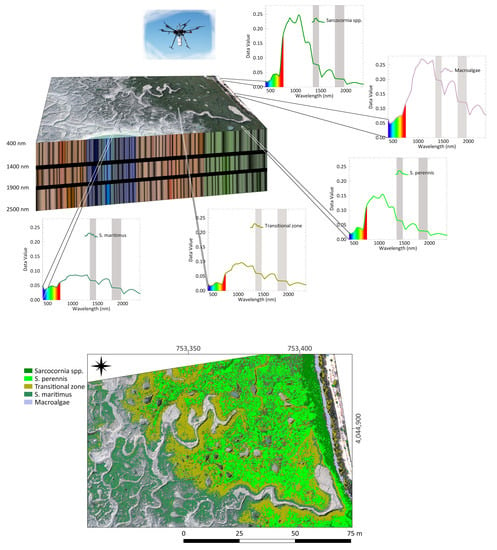
This work examines the potential of high spatial and spectral resolution UAV-HS data to accurately identify and differentiate the distribution of the salt marsh vegetation at the level of species. The specific goals are (1) to determine which is the appropriate UAV-HS dataset to map salt marsh vegetation; (2) to assess the separability of salt marsh interest classes; and (3) to estimate the elevation ranges of the detected species. These findings are expected to become a starting point for the early assessment of salt marsh degradation and help in the selection of areas for salt marsh rehabilitation or detection of the establishment and spread of alien species.

2. Materials and Methods

2.1. Site Description

Cadiz Bay hosts the southernmost European coastal wetland, located where the Mediterranean Sea, the Atlantic Ocean, and the continents of Europe and Africa converge (Figure 1). Located on the Atlantic coastline, precipitation, wind, and waves are influenced by large-scale oceanic weather systems that cross the North Atlantic [51]. Cadiz Bay is delimited by the tombolo of the city of Cadiz, with NNW-SSE orientation, and opens towards the Atlantic Sea to the north [52]. The entire bay is formed by two water bodies, the external and the inner bay, connected by tides through a narrow strait [53]. The external basin has depths up to 20 m, whereas the inner basin has a mean depth of about 2 m, and is sheltered from ocean waves [54]. The intertidal system of the bay is composed of natural salt marshes, salinas, mudflats, and an intricate network of tidal creeks [55]. The tidal regime is mesotidal semi-diurnal with a mean spring tidal range of 2.96 m [56].

The distribution of vegetation in the natural salt marshes of Cadiz Bay follows a conventional mid-latitude zonation [57], although the protective walls of the salinas frequently cut off the high marsh. The low marsh is mostly inhabited by Sporobolus maritimus, whereas the medium marsh is dominated by Sarcocornia spp., primarily Sarcocornia fruticosa (L.) A.J.Scott and Sarcocornia perennis (Mill.) A.J.Scott, and other halophytic species in lower abundance (Figure 2). Seagrass beds of Zostera noltei Hornem. and Cymodocea nodosa Asch., as well as patches of Zostera marina L., are found at the lower parts of the intertidal zone [53].

Our study area was selected in an area with a wide and well-developed natural salt marsh zonation, in the north-eastern corner of the inner bay [54].

2.2. UAV and Hyperspectral Sensor

This work was performed with a Matrice 600 hexacopter (DJI) (UAV from now) equipped with a co-aligned VNIR–SWIR hyperspectral (HS from now) system (Headwall Photonics), all property of the University of Cadiz [58].

The HS unit captures continuous information in the 400–2500 nm spectral range, (see [58] for further information). The HS instrument provides VNIR and SWIR data as separate files, but they can be stacked in a single hypercube containing the complete VNIR–SWIR information (see Section 2.4.2).

For data accuracy, the HS system includes an APX-15 GNSS-inertial solution (Trimble Applanix), and the UAV incorporates three built-in GPSs. These GPSs provide an accuracy of ±0.5 m and ±1.5 m in the vertical and horizontal, respectively. However, the post-processing of the APX-15 data increases accuracy to 0.02 m and 0.05 m, respectively.

2.3. UAV-Based Data Acquisition

Flight operations were conducted on 22 October 2021 between 10 am and 12 pm with a low tide of 1.3 m LAT (lowest astronomical tide), covering an area of 4.8 ha (Figure 1c). Clear weather ensured uniform lighting conditions for setting the flight and the sensor. The flight mission was planned with UgCS desktop, version 4.5 (SPH engineering). The flight altitude was set at 120 m and the speed at 5 m/s to ensure radiometric quality. This HS sensor does not require frontal overlap, but a 40% lateral overlap was set to assure the subsequent reconstruction of the orthomosaic. The sensor was calibrated by obtaining a reference spectrum in the 400–1700 nm range from a radiometrically calibrated tarp (3 × 3 m). A Reach RS2+ RTK GNSS antenna (EMLID) was used as a base station (see Section 2.4.1). This antenna allows for obtaining more precise results with accuracies of 4 mm + 1 ppm and 8 mm + 1 ppm, in horizontal and vertical measurements, respectively.

2.4. Hyperspectral Data Processing

This section summarizes the processing to generate the HS products (Figure 3). The processing was performed with ENVI, v. 5.3.6 (L3Harris Geospatial Solutions, Inc., Broomfield, CO, USA -.), whereas QGis, v. 3.26.3 (QGIS Development Team) was used for the visualization and handling of raster deliverables. The projected coordinate system used in this work was the ETRS89, UTM zone 29 N (EPSG:25829).

2.4.1. Hyperspectral Pre-Processing

Data from the APX-15 is processed with the POSPac UAV software, v. 8.9 (Trimble Applanix), using the data from the antenna to improve accuracy and create the smoothed best-estimated trajectory (SBET). This file, with root mean square errors (RMSEs) within 0.02–0.05 m, is used for the orthorectification of the hypercubes (Figure 3(0)).

The VNIR and SWIR data cubes are processed separately using SpectralView, v 3.2.0 (Headwall Photonics) as follows: (1) raw data is transformed to radiance (Figure 3(1)) by subtracting the dark reference from the digital numbers (DNs). The dark spectrum is collected in the field by covering the sensor lens after the mission and is considered sensor noise; (2) the reflectance correction is the conversion of radiance to reflectance (Figure 3(2)). This step is used to build a line of best fit between the radiance of the HS sensor and the reflectance measured on the radiometric tarp [59,60]; (3) the orthorectification (Figure 3(3)) is performed by combining a precision DSM and the SBET from step 1. For this operation, a DSM from Curcio et al. [34] was used, with 0.05 m/pixel resolution and 0.01 m mean accuracy; (4) the processed VNIR and SWIR hypercubes are stitched together (mosaicking, Figure 3(4)) into a single final mosaic that is orthorectified and georeferenced.

2.4.2. Hyperspectral Post-Processing

Atmospheric correction is not required when flying at a maximum altitude of 120 m. Once mosaicked, VNIR and SWIR hypercubes are stacked into a single file and the wavelengths associated with water vapour absorbance (i.e., 1350–1460 nm; 1790–1960 nm; 2350–2500 nm [28]) are excluded, resulting in an orthomosaic with 418 exploitable bands (Figure 3(5)).

The Normalized Difference Vegetation Index (NDVI) is used to discriminate the presence of vegetation in the study area (Figure 3(6)) and generate the training set for the final classification step (see Section 2.5). The NDVI map layer is calculated according to Equation (1):

NDVI = (NIR − RED)/(NIR + RED)

(1)

with NIR and RED as the near-infrared and red bands centred at 860 nm and 649 nm, respectively. Very low NDVI values (0.1 and below) are associated with bare soil or water, moderate values (~0.3) correspond to shrub and grassland, and high values (0.6–1) are associated with high-density plants and healthy physiological conditions [61]. Since only shrub and grassland vegetation was considered for this work, the NDVI map layer was masked with a threshold of 0.3. The product of this step is a raster with only vegetation distribution.

2.4.3. Endmember Extraction

An endmember is a pure signature for a class [62] and they are essential for the classification of HS data. Pure signatures from hyperspectral imagery can be found using minimum noise fraction (MNF), the Pixel Purity Index (PPI), and endmember extraction techniques (Figure 3). The MNF maximises the noise-to-signal ratio and reduces dimensionality without sacrificing information [63] (Figure 3(7)). Most of the significant information is contained in the first MNF bands, which are used in successive processing, ignoring the rest of the bands containing only noise [64]. The PPI technique [65] searches for pure spectral signatures by identifying the pixels with the fewest mixed spectral signatures (Figure 3(8)). The PPI image locates the pure pixels of the scene, which will then be used to extract the spectra of the potential endmembers [66]. A region of interest (ROI) is a dataset sample considered important for a particular purpose [67]. In this case, the regions of interest (ROIs) contain the pixels with the pure spectra in the scene and are imported in the n-Dimensional Visualizer scatter plot (n-DV; Figure 3(9)). The n-DV is an ENVI tool for visualising the distribution of pixels in the n-D space (where n is the number of bands), allowing the purest pixels representing the spectral endmembers to be identified and clustered (Figure 3(10,11)). After these steps, the classification procedure can be carried out.

2.5. Classification

The classification process uses unsupervised and supervised algorithms to map the spatial location and abundance of each endmember spectrum. The relevant MNF bands are the input for the ISODATA algorithm (Figure 3(12)), which iteratively clusters the pixels using the least distance approach [68]. The result is a first classified image based on the inherent spectral information of the dataset, with each class represented by a different endmember.

The next level of classification is produced by the spectral angle mapper (SAM) algorithm (Figure 3(13)), which calculates the angle between two spectra to identify their spectral similarity based on a maximum angle threshold [69]. This threshold is set to 0.1 radians to minimize spectral mixing issues. This algorithm uses the endmembers of the unsupervised classification to classify.

The last algorithm selected in this study is the support vector machine (SVM) (Figure 3(15)), selected because of the good results it produces with heterogeneous, complex, and noisy data [70]. The SVM separates the classes using a training set with class samples (i.e., support vectors) [71], with every class represented by an ROI. In this case, ROIs are generated based on three sources of information: (1) the unsupervised classification; (2) the SAM-classified image; (3) the NDVI map (Figure 3(14)).

2.6. Spectral Analysis

To verify that UAV-HS datasets can differentiate vegetation at the species level in salt marshes, the separability of the spectral signatures of the classifications must be tested. This was analysed through spectral transformations. In addition, the usefulness of new spectral indices for the separation of species is explored, using the relevant wavelengths highlighted by the spectral transformations to generate them.

2.6.1. Continuum Removal and Second-Order Derivative

The differences in absorption and reflection spectra between vegetation species can be very small, making classification difficult. Spectral transformation, such as continuum removal (CR) and derivative spectroscopy, have the potential to amplify small differences [28,42,72]. CR is used to normalize the spectra, and sometimes this is enough to highlight differences in absorption and reflection spectra [73]. The second-order derivative method (2nd derivative from now) emphasises the small differences in absorption peaks associated with biochemical properties, allowing for the identification of different species [28,74]. To enhance the signal-to-noise ratio and extract additional hidden spectral features, the 2nd derivative spectrum is filtered using a boxcar average smoothing. All transformed spectra are analysed in four separated wavelength windows: visible region (VIS, 400–700 nm), near-infrared region (NIR, 700–1000 nm), and two regions of short-infrared (SWIR1, 1000–1800 nm; SWIR2, 1800–2350 nm).

2.6.2. Spectral Indices (SI)

New spectral indices (SI) have been constructed from the most outstanding absorption and reflectance features (peaks and valleys of the 2nd derivative, respectively) of the transformed spectrum. These indices can emphasize the distribution of different vegetation species in the salt marsh. Each SI is calculated according to Equation (2) (known as the normalized difference):

SI_B2-B1 = (B2 − B1)/(B2 + B1)

(2)

where SI_B2-B1 is the calculated spectral index, B1 is the wavelength presenting the absorption feature, and B2 is the wavelength presenting the reflectance feature. This type of equation brings out characteristics not initially visible.

2.7. Validation

2.7.1. Spectral Signatures

The spectral responses of our study area were previously studied in 2014–2015 (FAST project, [75]). In the FAST project, each sampling point was a 1 × 1 m area where five reflectance measurements were made using a field hyperspectral radiometer for the VNIR range (400–1000 nm).

The FAST spectra measurements are utilised here as a reference spectral library to identify species based on their spectral features. All spectra from our classification results are compared to the library using the Spectral Analyst tool from ENVI. The similarities of our classification spectra to those in the library are calculated by providing a similarity score to each spectrum in the library, with the highest score considered the closest match (i.e., the most confident spectral similarity). This analysis considers only the wavelength range available in the FAST library (400–1000 nm).

2.7.2. Classification

Two methods are used to determine the SVM classification accuracy. The first one is the comparison of the classification results with the composition of species observed at 60 randomly sampled points in the study area. To buffer small errors associated with very precise locations, the species from the classification was determined as the prevalent class in a 15 cm diameter buffer area around each point.

The second method is the comparison with random pixels from other sources. In total, seven comparisons are performed from seven sets of random pixels. One set is obtained from the training ROIs. The other six sets are generated from the unsupervised classified image using different sampling methods: (1) two sets are generated with stratified-proportionate samples (SP), with sizes directly related to the size of the classes; (2) two sets of equalized samples (Eq), with fixed size regardless of the class size; and (3) two sets of random samples (R), using 10% and 20% of the total pixels.

For each comparison, the accuracy is determined from (1) the overall accuracy, calculated by counting the correctly classified values and dividing by the total number of values; (2) producer accuracy, which measures the likelihood of correctly classifying a value into each class; (3) user accuracy, which shows the likelihood that a prediction belongs to the correct class. Each probability is determined by dividing the proportion of correct values by the total number of values in a class.

2.8. Elevation of Species Distribution

Once the vegetation classes are confirmed, their elevation distribution is assessed using a DEM with 0.24 m/pixel resolution and a mean accuracy of 0.04 m [34]. The corresponding elevations are extracted for each class using 5 cm sampling grids. After removing outliers, the elevation of each class is characterized using a set of statistical parameters (i.e., minimum, maximum, median, and mode).

3. Results

3.1. Classification Result

For the SVM supervised classification, a total of 15 ROIs were recognized, corresponding to 15 classes, 7 of them associated with vegetation classes. However, only four of these classes are within the salt marsh horizons considered in this work. Regarding the other three vegetation classes, one has been associated with macrophyte debris deposited in the uppermost zone of the salt marsh by an extreme high tide event, and the other two with the typical vegetation of the saline wall. These last two classes are outside the scope of this work and, therefore, will not be taken into consideration. Nevertheless, it is interesting that they can be distinguished from salt marsh species.

Of the 4.8 ha of surveyed salt marsh, the spatial mapping of the endmembers estimates a vegetation cover of 14.7% of the area. These species are distributed parallel to the mean sea line and in different elevation ranges.

In this work, the vegetation classes within the salt marsh horizons include four classes of salt marsh species and a fifth class associated with macroalgal debris. From high to low elevations, the distribution of these classes is macroalgal debris deposits first, followed by vegetation 1 and 2 in the mid-horizon, vegetation 3 within the transition zone, and vegetation 4 in the low horizon. The area covered by these classes is 2.9%, 9.2%, 34.3%, 28.9%, and 24.9% of the vegetated area, respectively (Figure 4).

3.2. Spectral Analysis

The four marsh vegetation classes show typical plant spectral curves (Figure 5). The peaks of each class are located at the same wavelength (±5 nm), presenting only quantitative differences. The macroalgae class showed clear divergences from this pattern. First, the strong absorption peak in the red region (peak 3 in Figure 5) is less pronounced than in plant classes. It also lacks the absorption peak at 943 nm (peak 6 in Figure 5). There is a significant increase in reflectance from the red-edge region to the SWIR1 region (i.e., 700–1300 nm), and also higher reflectance in entire the SWIR region (1000–2350 nm) (Figure 5,

Table 1. Wavelengths of the absorption peaks detected in the spectral signature of the marsh vegetation classes of Cadiz Bay. The numbers in the column headers correspond to the peaks indicated in Figure 5. Units: nm.

Class\Peak	(1)	(2)	(3)	(4)	(5)	(6)	(7)	(8)	(9)	(10)
Macroalgae	447	500	669	776	864	-	997	1182	1523	2025
Vegetation 1	443	492	669	776	860	943	991	1206	1523	2025
Vegetation 2	447	487	669	776	860	943	991	1194	1523	2025
Vegetation 3	447	487	669	776	864	943	997	1188	1523	2025
Vegetation 4	443	483	669	776	864	943	997	1182	1523	2025

).

The 2nd derivative transformation accentuated small differences not previously observed in the reflectance curves (Figure A1, Figure A2, Figure A3 and Figure A4). These effects are more pronounced in the SWIR1 region, and the variations between 2013 and 2329 nm (SWIR2 region) are particularly notable.

The spectral indices (SI) were constructed with the significant absorbance peaks at 1057, 1110, 1152, 1182, 1260, and 1331 nm, generating SI_1152-1110, SI_1331-1260, SI_1182-1057, and SI_1523-1290. These indices may show differences that can be attributed to biophysical differences in vegetation (Figure 6).

3.3. Validation

According to the scores obtained, vegetation 1 and 2 classes may represent Sarcocornia spp., while vegetation 4 class may correspond to Sporobolus maritimus. Vegetation 3 class has been attributed to areas of overlap of different proportions of these species (i.e., the transition zone).

The categories identified at the field reference points were Sarcocornia, Salicornia, and transition zones only. However, distinguishing between Sarcocornia and Salicornia species in the field is very challenging and misidentifications can be expected [76]. The accuracy of the classification was estimated to be 46% but increased to 73% when considering that Sarcocornia and Salicornia could be mistaken for each other in the field. When comparing the classification to the sets of random pixels, the accuracy ranges from 92 to 96% (

Table 2. Overall accuracy of the HS image classification. The accuracy is estimated by comparison with field measurements, random samples generated from ROIs, and other groups of random samples (Eq250, Eq500, R10, R20, Sp10, Sp20). Eq250 and Eq500 are the equalized samples groups using 250 and 500 pixels respectively for each class as reference; R10 and R20 are the random samples groups using 10% and 20 % of total pixels as reference respectively; Sp10 and Sp20 are the stratified-proportionate samples groups using 10% and 20 % of total pixels as reference, respectively.

Estimation Method	Accuracy
Eq250	92.5%
Eq500	92.4%
Field measurement	46–73%
ROIs	95.9%
R10	95.6%
R20	95.7%
Sp10	95.9%
Sp20	95.8%

).

3.4. Elevation Range of Identified Species

Vegetation 1 class (identified as a short Sarcocornia spp. or a Salicornia spp.) is included within the elevation range of the vegetation 2 class (identified as S. perennis) (

Table 3. Estimated elevation range for each salt marsh vegetation class identified in Cadiz Bay. S. perennis: Sarcocornia perennis; S. maritimus: Sporobolus maritimus. Figure A5 shows the frequency distribution of the extracted values for each class; Q: quantile.

Class	Specie	0.05 Q	0.25 Q	0.5 Q	0.75 Q	0.95 Q	Mode
Macroalgae	Macroalgae	1.13	2.54	2.75	3.43	3.77	2.81
Vegetation 1	Salicornia spp. o Sarcocornia spp.	2.34	2.53	2.62	2.69	2.75	2.67
Vegetation 2	S. perennis	2.30	2.56	2.67	2.74	2.80	2.79
Vegetation 3	Transitional	1.91	2.26	2.42	2.58	2.78	2.00
Vegetation 4	S. maritimus	1.22	1.76	1.94	2.10	2.35	1.68

). The two classes spread across the same elevation range, but the mode of their elevation range is different, with 2.67 m vs 2.79 m for vegetation 1 and 2, respectively. The transitional class (vegetation 3) extended from 1.91 m to 2.78 m, narrowing to 2.26–2.58 m for Q1–Q3. The S. maritimus (vegetation 4) covers a range between 1.22 m and 2.35 m (1.76–2.10 m for Q1–Q3). Macroalgae have a bimodal distribution, with two accumulation zones located at 2.49–2.86 m and 3.35–3.84 m (Figure A5).

4. Discussion

The analyses of hyperspectral datasets from low and medium salt marsh areas in Cadiz Bay are adequate to identify vegetation distribution at the species level. Four plant classes distributed along the horizons of the salt marsh and one class of macrophyte debris were recognised. Three of the plant classes have been associated with monospecific vegetation (Sarcocornia spp., S. perennis, and S. maritimus), while a fourth class represents the mix of species typical of the convergence of distributions (i.e., transition zone). The results from this study are expected to be extrapolated to other mid-latitude tidal marshes since the low and medium tidal marshes of these latitudes usually present similar structural traits [75].

The performance of the SAM classification method is limited in areas with several species due to the mix of spectra [77]. However, this problem can be minimised by using the two supervised classification methods (SAM and SVM) in succession after performing hyperspectral processing procedures. The SVM supervised classification reached up to 98% accuracy, demonstrating its effectiveness in mapping land cover. When looking at the accuracy of individual classes, features such as water bodies and types of soil perfectly match the reference data. Focusing on vegetation classes, the highest accuracy is achieved by vegetation 1, vegetation 4 and macroalgae. The accuracy is lower, although still significant for the remaining classes (

Table A1. Report for the accuracy of the comparison of classification results to Eq250, the equalized samples groups using 250 pixels for each class as reference. The table summarizes the producer accuracy and user accuracy in percentage and pixels for each class.

Class	Class Name	Prod. Acc. (Percent)	User Acc. (Percent)	Prod. Acc. (Pixels)	User Acc. (Pixels)
ROI #1	Vegetation 1	98.00	98.00	245/250	245/250
ROI #2	Vegetation 2	74.80	87.38	187/250	187/214
ROI #3	Vegetation 3	66.80	81.07	167/250	167/206
ROI #4	Ponds with mpb	100.00	99.60	250/250	250/251
ROI #5	Vegetation 5	85.20	78.89	213/250	213/270
ROI #6	Vegetation 6	88.00	81.48	220/250	220/270
ROI #7	Soil	99.60	89.89	249/250	249/277
ROI #8	Soil with mph	98.40	94.62	246/250	246/260
ROI #9	Tidal channel	100.00	100.00	250/250	250/250
ROI #10	Saline	100.00	100.00	250/250	250/250
ROI #11	Ponds without water	90.40	97.84	226/250	226/231
ROI #12	Shallow water	99.60	100.00	249/250	249/249
ROI #13	Dry soil	100.00	100.00	250/250	250/250
ROI #14	Macroalgae	98.40	100.00	246/250	246/246
ROI #15	Vegetation 4	88.00	79.71	220/250	220/276

,

Table A2. Report for the accuracy of the comparison of classification results to Eq500, the equalized samples groups using 500 pixels for each class as reference. The table summarizes the producer accuracy and user accuracy in percentage and pixels for each class.

Class	Class Name	Prod. Acc. (Percent)	User Acc. (Percent)	Prod. Acc. (Pixels)	User Acc. (Pixels)
ROI #1	Vegetation 1	98.13	98.13	419/427	419/427
ROI #2	Vegetation 2	74.00	85.87	316/427	316/368
ROI #3	Vegetation 3	66.74	78.51	285/427	285/363
ROI #4	Ponds with mpb	100.00	100.00	427/427	427/427
ROI #5	Vegetation 5	84.31	77.25	360/427	360/466
ROI #6	Vegetation 6	84.78	81.35	362/427	362/445
ROI #7	Soil	99.77	90.83	426/427	426/469
ROI #8	Soil with mph	98.83	96.57	422/427	422/437
ROI #9	Tidal channel	100.00	100.00	427/427	427/427
ROI #10	Saline	100.00	100.00	427/427	427/427
ROI #11	Ponds without water	90.87	99.49	388/427	388/390
ROI #12	Shallow water	100.00	100.00	427/427	427/427
ROI #13	Dry soil	100.00	100.00	427/427	427/427
ROI #14	Macroalgae	98.83	99.29	422/427	422/425
ROI #15	Vegetation 4	89.93	80.00	384/427	384/480

,

Table A3. Report for the accuracy of the comparison of classification results to random samples generated from ROIs. The table summarizes the producer accuracy and user accuracy in percentage and pixels for each class.

Class	Class Name	Prod. Acc. (Percent)	User Acc. (Percent)	Prod. Acc. (Pixels)	User Acc. (Pixels)
ROI #1	Vegetation 1	97.88	97.13	508/519	508/523
ROI #2	Vegetation 2	73.80	80.25	386/523	386/481
ROI #3	Vegetation 3	66.61	72.40	417/626	417/576
ROI #4	Ponds with mpb	100.00	99.07	427/427	427/431
ROI #5	Vegetation 5	82.86	85.66	986/1190	986/1151
ROI #6	Vegetation 6	86.01	82.09	793/922	793/966
ROI #7	Soil	99.20	98.63	4734/4772	4734/4800
ROI #8	Soil with mph	98.29	97.87	1838/1870	1838/1878
ROI #9	Tidal channel	100.00	100.00	5997/5997	5997/5997
ROI #10	Saline	100.00	99.95	1915/1915	1915/1916
ROI #11	Ponds without water	90.67	93.71	447/493	447/477
ROI #12	Shallow water	99.87	100.00	767/768	767/767
ROI #13	Dry soil	100.00	100.00	508/508	508/508
ROI #14	Macroalgae	98.56	99.39	821/833	821/826
ROI #15	Vegetation 4	89.75	83.13	744/829	744/895

,

Table A4. Report for the accuracy of the comparison of classification results to R10, the random samples group using 10% of total pixels as reference. The table summarizes the producer accuracy and user accuracy in percentage and pixels for each class.

Class	Class Name	Prod. Acc. (Percent)	User Acc. (Percent)	Prod. Acc. (Pixels)	User Acc. (Pixels)
ROI #1	Vegetation 1	98.39	96.83	61/62	61/63
ROI #2	Vegetation 2	67.44	78.38	29/43	29/37
ROI #3	Vegetation 3	67.92	63.16	36/53	36/57
ROI #4	Ponds with mpb	100.00	100.00	40/40	40/40
ROI #5	Vegetation 5	78.38	83.65	87/111	87/104
ROI #6	Vegetation 6	83.91	79.35	73/87	73/92
ROI #7	Soil	98.82	97.66	501/507	501/513
ROI #8	Soil with mph	100.00	98.32	176/176	176/179
ROI #9	Tidal channel	100.00	100.00	601/601	601/601
ROI #10	Saline	100.00	100.00	188/188	188/188
ROI #11	Ponds without water	79.25	93.33	42/53	42/45
ROI #12	Shallow water	98.90	100.00	90/91	90/90
ROI #13	Dry soil	100.00	100.00	47/47	47/47
ROI #14	Macroalgae	98.55	100.00	68/69	68/68
ROI #15	Vegetation 4	90.11	86.32	82/91	82/95

,

Table A5. Report for the accuracy of the comparison of classification results to R20, the random samples group using 20% of total pixels as reference. The table summarizes the producer accuracy and user accuracy in percentage and pixels for each class.

Class	Class Name	Prod. Acc. (Percent)	User Acc. (Percent)	Prod. Acc. (Pixels)	User Acc. (Pixels)
ROI #1	Vegetation 1	99.14	97.46	115/116	115/118
ROI #2	Vegetation 2	65.98	76.19	64/97	64/84
ROI #3	Vegetation 3	65.04	74.77	80/123	80/107
ROI #4	Ponds with mpb	100.00	96.43	81/81	81/84
ROI #5	Vegetation 5	83.40	84.45	201/241	201/238
ROI #6	Vegetation 6	88.18	84.04	179/203	179/213
ROI #7	Soil	99.04	98.21	933/942	933/950
ROI #8	Soil with mph	96.49	98.89	357/370	357/361
ROI #9	Tidal channel	100.00	100.00	1162/1162	1162/1162
ROI #10	Saline	100.00	99.75	398/398	398/399
ROI #11	Ponds without water	90.82	89.90	89/98	89/99
ROI #12	Shallow water	100.00	100.00	170/170	170/170
ROI #13	Dry soil	100.00	100.00	77/77	77/77
ROI #14	Macroalgae	97.31	99.45	181/186	181/182
ROI #15	Vegetation 4	91.95	82.47	160/174	160/194

,

Table A6. Report for the accuracy of the comparison of classification results to Sp10, the stratified-proportionate samples group using 10% of total pixels as reference. The table summarizes the producer accuracy and user accuracy in percentage and pixels for each class.

Class	Class Name	Prod. Acc. (Percent)	User Acc. (Percent)	Prod. Acc. (Pixels)	User Acc. (Pixels)
ROI #1	Vegetation 1	92.31	97.96	48/52	48/49
ROI #2	Vegetation 2	69.23	76.60	36/52	36/47
ROI #3	Vegetation 3	71.43	66.18	45/63	45/68
ROI #4	Ponds with mpb	100.00	100.00	43/43	43/43
ROI #5	Vegetation 5	80.67	87.27	96/119	96/110
ROI #6	Vegetation 6	88.04	81.82	81/92	81/99
ROI #7	Soil	99.58	98.75	475/477	475/481
ROI #8	Soil with mph	98.40	98.40	184/187	184/187
ROI #9	Tidal channel	100.00	100.00	600/600	600/600
ROI #10	Saline	100.00	100.00	192/192	192/192
ROI #11	Ponds without water	89.80	95.65	44/49	44/46
ROI #12	Shallow water	100.00	100.00	77/77	77/77
ROI #13	Dry soil	100.00	100.00	51/51	51/51
ROI #14	Macroalgae	98.80	98.80	82/83	82/83
ROI #15	Vegetation 4	90.36	86.21	75/83	75/87

and

Table A7. Report for the accuracy of the comparison of classification results to Sp20, the stratified-proportionate samples group using 20% of total pixels as reference. The table summarizes the producer accuracy and user accuracy in percentage and pixels for each class.

Class	Class Name	Prod. Acc. (Percent)	User Acc. (Percent)	Prod. Acc. (Pixels)	User Acc. (Pixels)
ROI #1	Vegetation 1	98.08	97.14	102/104	102/105
ROI #2	Vegetation 2	77.14	80.20	81/105	81/101
ROI #3	Vegetation 3	65.60	70.09	82/125	82/117
ROI #4	Ponds with mpb	100.00	97.70	85/85	85/87
ROI #5	Vegetation 5	81.93	86.67	195/238	195/225
ROI #6	Vegetation 6	87.50	82.14	161/184	161/196
ROI #7	Soil	99.06	98.23	945/954	945/962
ROI #8	Soil with mph	97.59	97.86	365/374	365/373
ROI #9	Tidal channel	100.00	100.00	1199/1199	1199/1199
ROI #10	Saline	100.00	100.00	383/383	383/383
ROI #11	Ponds without water	85.86	90.43	85/99	85/94
ROI #12	Shallow water	100.00	100.00	154/154	154/154
ROI #13	Dry soil	100.00	100.00	102/102	102/102
ROI #14	Macroalgae	98.80	100.00	165/167	165/165
ROI #15	Vegetation 4	89.76	84.66	149/166	149/176

). The spectral signature of the transition zone (vegetation 3 class), which is a variable mixture of plant species and, therefore, a variable mix of spectra, makes this class the lowest in accuracy (63.16%). Since the training dataset used to produce the map (i.e., ROIs) determines the quality of the algorithm classification, a single ROI for transition zones is considered insufficient to accurately represent the variability associated with different levels of species mix. Still, the overall accuracy provided by our UAV-HS approach is higher than previous classification attempts. Rasel et al. [31] obtained a 43% overall accuracy from space-borne hyperspectral data with 30 m spatial resolution. Rajakumari et al. [28] combined satellite multispectral data and ground spectrometric measurements, achieving 65.8% to 73.55% accuracy for the vegetation and land cover spectral signatures, respectively.

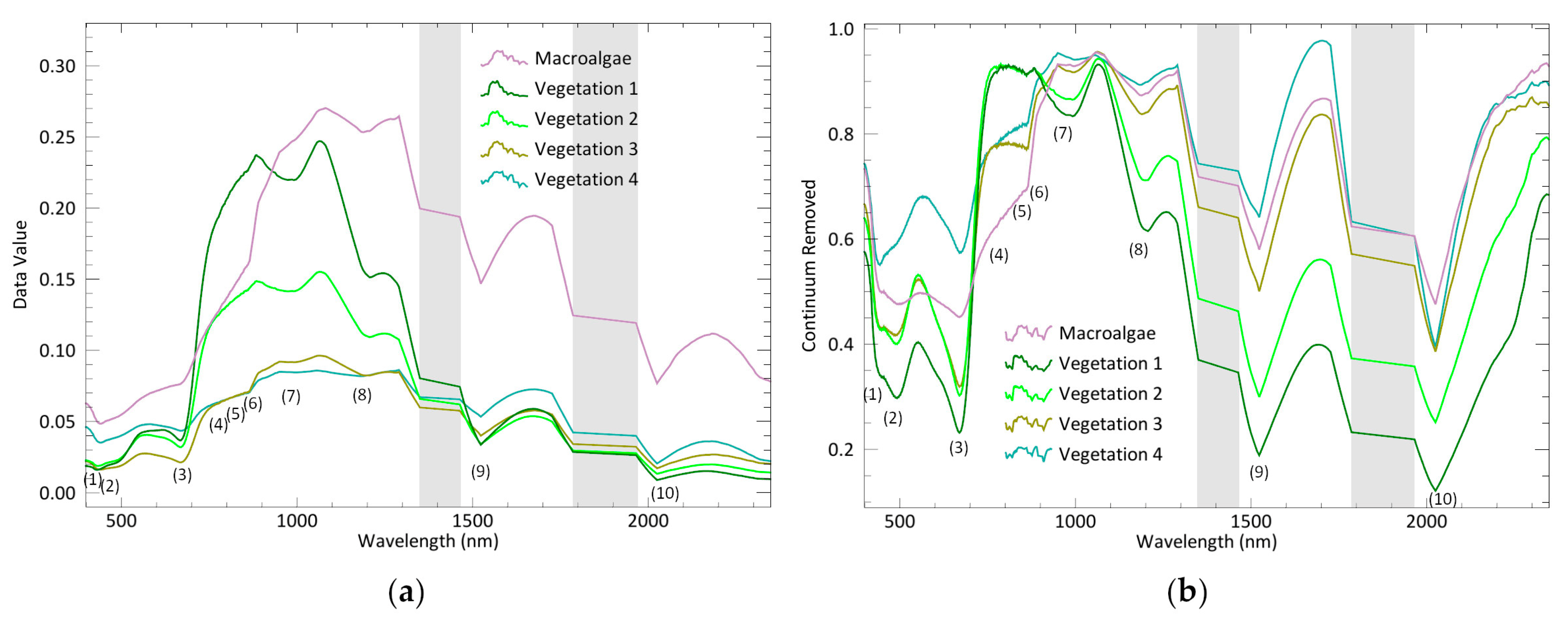
Among the endmembers extracted from Cadiz Bay salt marshes, four exhibit the typical plant pattern, while one shows the macroalgae response with distinct peaks and slopes of the reflectance spectrum. Chlorophyll a (Chl-a), found in both plants and macroalga, determines a typical absorption peak at 669 nm. However, this feature is smoothed in the spectral signature of macroalgae (Figure 5), maybe due to its yellowish-brown colour related to the fucoxanthin content [78]. The class of macroalgae in this study corresponds to debris deposited by an extreme flood event at an elevated position far removed from ordinary tidal cycles. This material dries and decomposes, resulting in high reflectance values in the NIR–SWIR, a typical region where water often attenuates spectral signatures [79]. The reflectance curves of the four remaining classes do not differ much from each other, the only significant variations being in the peak intensity. However, the continuum removal transformation enhances different responses in the 740–864 region, with opposite slopes in the curve between 882 and 949 nm (Figure 7). These findings lead to the acceptance of vegetation 1 and 2 as the spectral signatures of Sarcocornia species in the medium marsh horizon, and vegetation 3 and 4 as the signatures of species distributed in the transition and the low marsh, respectively.

Different species of Sarcocornia dominate the medium marsh in Cadiz Bay [55,57]. However, because they are morphologically similar to Salicornia species, it is very challenging to distinguish them in the field when they coexist, and misidentification can occur [76]. As revealed by the CR spectra, vegetation 1 and 2 differ almost only in the intensity of the peaks, demonstrating optical similarities. However, the 2nd derivative analysis reveals that two groups of halophytes are spectrally distinct (Figure A1, Figure A2, Figure A3 and Figure A4), with these spectral differences resulting from biochemical variations between salt marsh species [28]. The pigment content, canopy structure, leaf area and leaf structure all have an impact on the visible region of the reflectance spectrum of plant canopies [42]. The 2nd derivative of our reflectance curves shows differences in the blue and red regions at wavelengths associated with the chlorophyll and xanthophyll peaks [74]. However, our work shows that the largest 2nd derivative peaks are in the SWIR region, and many of them coincide with water absorption wavelengths. Water absorption bands are present at 900 and 967 nm (the water band index [80]), in the 1150–1260 nm region [81] and in the 1450–1940 nm region [82]. Salinity in soils and vegetation is also detectable in the SWIR region [83,84], and Kumar et al. [85] proposed a SWIR-based vegetation index to detect changes in vegetation cover from satellites. All these previous works support our conclusion that SWIR, with its highest spectral variability, is a suitable region to discriminate plant species from salt marshes. The SI established here can reveal differences in the canopy cover (Figure 6), proving that UAV-HS is able to detect variations in canopy cover at the species level. The great advantages of UAVs are the high spatial and temporal resolutions of their products, as well as greater flexibility and lower cost when compared to satellite products. This allows, for example, data collection immediately after an extreme event and then periodically afterwards, providing key data to assess the ability of dynamic systems, such as salt marshes, to return to previous states (or resilience).

The horizon of the low salt marsh in Cadiz Bay is dominated by S. maritimus [55]. Its shoot structure and density allow the soil to be exposed, resulting in a mixed spectrum of soil and plant responses that is very similar to the spectral signature of soil with microphytobenthos. This problem may result in misinterpretations when using low spatial resolution sensors [1]. The higher spatial resolution (5 cm/pixel) offered by UAVs not only prevents this issue, but also reduces the occurrence of mixed spectral signatures due to the reduced pixel size. The comparison of the spectral responses of the S. maritimus class (vegetation 4) with the soil classes (Figure 8) shows that the influence of the soil is inevitable. However, S. maritimus habitats and soil with microphytobenthos can be distinguished by CR and 2nd derivative transformations in the red-edge and SWIR2 regions (Figure 9). This demonstrates that these two habitats can be distinguished in UAV-HS datasets, allowing for more precise mapping of S. maritimus and microphytobenthos soil and minimizing overestimation/underestimation issues for these categories.

The zonation of salt marsh plant species depends on elevation, tidal regime, and the gradient of environmental variables, such as salinity, redox potential, soil N, clay, and organic matter content, as well as interspecific relationships [2,86,87,88]. According to Redondo-Gomez et al. [89], in SW Spain, S. perennis subsp. perennis occupies from 2.26 to 2.84 m LAT, and S. perennis subsp. alpini from 2.84 to 3.65 m LAT. Our results agree with these findings, showing that Sarcocornia spp. inhabit the salt marsh horizon between 2.30 m and 2.80 m LAT. Previous studies have described S. fruticose and S. perennis as dominant species in the salt marshes of Cadiz Bay [55]. Unfortunately, the spectral library available in our study area (FAST project, [75]) does not specify which Sarcocornia taxa were measured. However, due to differences in the SWIR region, our results suggest that two Sarcocornia taxa coexist in the medium salt marsh horizon. Differences in this part of the spectrum have previously been related to differences in the salinity [84], suggesting that soil salinity may be playing a role in the zonation of Cadiz Bay tidal marshes. Although the elevation ranges for vegetation 1 and 2 overlap, suggesting a similar ecological niche, their different mode (2.67 m for vegetation 1 vs 2.79 m for vegetation 2, Table 3) indicate a shift in the optimum range of environmental conditions between the two groups, supporting the existence of two species. Both histograms are left skewed, indicating that these species can populate lower elevations despite performing better at higher positions. As a result of our findings, some resilience is expected in these habitats under sea level rise scenarios.

Regarding the accumulations of macroalgae, the decomposition of these accumulations of organic matter alters the availability of oxygen and the redox potential in the sediments, which could have negative consequences for multiple trophic levels if their incidence increases significantly [90,91]. Understanding the local carbon cycle and the dynamic of the system also requires mapping where macroalgae are deposited [78,91]. In Cadiz Bay, Sarcocornia spp. and S. maritimus overlap in a narrow area here called the transition zone (vegetation 3). This class has problems with accuracy mainly because of the wide variety of spectral responses due to the different proportions of Sarcocornia spp. and S. maritimus. Future studies may include more classes for the transition zone, but they will need careful spectral analysis to investigate the spectral response associated with specific proportions of the dominant species.

5. Conclusions

This study demonstrates the potential of UAV-HS technology to identify and map the distribution of plant species in salt marshes, using canopy reflectance information. Salt marsh plant species have very similar spectral shapes. However, hyperspectral technology is capable of detecting spectral differences associated with the water content and salinity of salt marsh plant tissues. The continuum removal and 2nd derivative transformations can detect hidden spectral features in reflectance curves, which can separate plant species with satisfactory accuracy. The classification map obtained through a supervised process reached up to 98% accuracy. The availability of an accurate DEM allows for the estimation of the preferred elevation range for each specie from the distribution of the corresponding classes. The overlap of species distribution generates mixes of spectra with a large variability associated with different species proportions. Future research may reduce these uncertainties but will require an increase in the number of associated classes.

Vegetation distribution is a key indicator in determining the health of salt marshes. The ability to monitor changes in these distributions will improve our understanding of salt marsh dynamics, our modelling capacity to assess responses to sea level rise, and help stakeholders manage these complicated, vulnerable, and valuable ecosystems. UAV-HS data can be used to evaluate salt marsh vulnerability and strengthen conservation efforts by defining critical areas for conservation and examining pressures on crucial ecosystem services, such as blue carbon.

References

1. Belluco, E.; Camuffo, M.; Ferrari, S.; Modenese, L.; Silvestri, S.; Marani, A.; Marani, M. Mapping Salt-Marsh Vegetation by Multispectral and Hyperspectral Remote Sensing. Remote. Sens. Environ. 2006, 105, 54–67. [Google Scholar] [CrossRef]
2. Veldhuis, E.R.; Schrama, M.; Staal, M.; Elzenga, J.T.M. Plant Stress-Tolerance Traits Predict Salt Marsh Vegetation Patterning. Front. Mar. Sci. 2019, 5, 501. [Google Scholar] [CrossRef] [Green Version]
3. Adam, P. Saltmarsh Ecology; Cambridge University Press: Cambridge, UK, 1990. [Google Scholar]
4. Duarte, C.M.; Losada, I.J.; Hendriks, I.E.; Mazarrasa, I.; Marbá, N. The Role of Coastal Plant Communities for Climate Change Mitigation and Adaptation. Nat. Clim. Chang. 2013, 3, 961–968. [Google Scholar] [CrossRef] [Green Version]
5. McLeod, E.; Chmura, G.L.; Bouillon, S.; Salm, R.; Björk, M.; Duarte, C.M.; Lovelock, C.E.; Schlesinger, W.H.; Silliman, B.R. A Blueprint for Blue Carbon: Toward an Improved Understanding of the Role of Vegetated Coastal Habitats in Sequestering CO2. Front. Ecol. Environ. 2011, 9, 552–560. [Google Scholar] [CrossRef] [PubMed] [Green Version]
6. Möller, I.; Kudella, M.; Rupprecht, F.; Spencer, T.; Paul, M.; van Wesenbeeck, B.K.; Wolters, G.; Jensen, K.; Bouma, T.J.; Miranda-Lange, M.; et al. Wave Attenuation over Coastal Salt Marshes under Storm Surge Conditions. Nat. Geosci. 2014, 7, 727–731. [Google Scholar] [CrossRef] [Green Version]
7. Wang, F.; Sanders, C.J.; Santos, I.R.; Tang, J.; Schuerch, M.; Kirwan, M.L.; Kopp, R.E.; Zhu, K.; Li, X.; Yuan, J.; et al. Global Blue Carbon Accumulation in Tidal Wetlands Increases with Climate Change. Natl. Sci. Rev. 2021, 8, nwaa296. [Google Scholar] [CrossRef] [PubMed]
8. Davy, A.J.; Brown, M.J.H.; Mossman, H.L.; Grant, A. Colonization of a Newly Developing Salt Marsh: Disentangling Independent Effects of Elevation and Redox Potential on Halophytes. J. Ecol. 2011, 99, 1350–1357. [Google Scholar] [CrossRef]
9. Janousek, C.N.; Folger, C.L. Variation in Tidal Wetland Plant Diversity and Composition within and among Coastal Estuaries: Assessing the Relative Importance of Environmental Gradients. J. Veg. Sci. 2014, 25, 534–545. [Google Scholar] [CrossRef]
10. Al Hassan, M.; Chaura, J.; López-Gresa, M.P.; Borsai, O.; Daniso, E.; Donat-Torres, M.P.; Mayoral, O.; Vicente, O.; Boscaiu, M. Native-Invasive Plants vs. Halophytes in Mediterranean Salt Marshes: Stress Tolerance Mechanisms in Two Related Species. Front. Plant Sci. 2016, 7, 473. [Google Scholar] [CrossRef] [Green Version]
11. Minden, V.; Andratschke, S.; Spalke, J.; Timmermann, H.; Kleyer, M. Plant Trait-Environment Relationships in Salt Marshes: Deviations from Predictions by Ecological Concepts. Perspect. Plant Ecol. Evol. Syst. 2012, 14, 183–192. [Google Scholar] [CrossRef]
12. Eleuterius, L.N.; Eleuterius, C.K. Tide Levels and Salt Marsh Zonation. Bull. Mar. Sci. 1979, 29, 394–400. [Google Scholar]
13. Roozen, A.J.M.; Westhoff, V. A Study on Long-Term Salt-Marsh Succession Using Permanent Plots. Vegetatio 1985, 61, 23–32. [Google Scholar] [CrossRef]
14. Murray, N.J.; Phinn, S.R.; DeWitt, M.; Ferrari, R.; Johnston, R.; Lyons, M.B.; Clinton, N.; Thau, D.; Fuller, R.A. The Global Distribution and Trajectory of Tidal Flats. Nature 2019, 565, 222–225. [Google Scholar] [CrossRef] [PubMed]
15. Lowe, M.R.; Peterson, M.S. Effects of Coastal Urbanization on Salt-Marsh Faunal Assemblages in the Northern Gulf of Mexico. Mar. Coast. Fish. 2014, 6, 89–107. [Google Scholar] [CrossRef] [Green Version]
16. Schuerch, M.; Spencer, T.; Temmerman, S.; Kirwan, M.L.; Wolff, C.; Lincke, D.; McOwen, C.J.; Pickering, M.D.; Reef, R.; Vafeidis, A.T.; et al. Future Response of Global Coastal Wetlands to Sea-Level Rise. Nature 2018, 561, 231–234. [Google Scholar] [CrossRef] [PubMed] [Green Version]
17. Xin, P.; Wilson, A.; Shen, C.; Ge, Z.; Moffett, K.B.; Santos, I.R.; Chen, X.; Xu, X.; Yau, Y.Y.Y.; Moore, W.; et al. Surface Water and Groundwater Interactions in Salt Marshes and Their Impact on Plant Ecology and Coastal Biogeochemistry. Rev. Geophys. 2022, 60, e2021RG000740. [Google Scholar] [CrossRef]
18. Fagherazzi, S.; Mariotti, G.; Leonardi, N.; Canestrelli, A.; Nardin, W.; Kearney, W.S. Salt Marsh Dynamics in a Period of Accelerated Sea Level Rise. J. Geophys. Res. Earth Surf. 2020, 125, e2019JF005200. [Google Scholar] [CrossRef]
19. Alizad, K.; Hagen, S.C.; Medeiros, S.C.; Bilskie, M.V.; Morris, J.T.; Balthis, L.; Buckel, C.A. Dynamic Responses and Implications to Coastal Wetlands and the Surrounding Regions under Sea Level Rise. PLoS ONE 2018, 13, e0205176. [Google Scholar] [CrossRef] [Green Version]
20. Kirwan, M.L.; Mudd, S.M. Response of Salt-Marsh Carbon Accumulation to Climate Change. Nature 2012, 489, 550–553. [Google Scholar] [CrossRef]
21. Narayan, S.; Beck, M.W.; Wilson, P.; Thomas, C.J.; Guerrero, A.; Shepard, C.C.; Reguero, B.G.; Franco, G.; Ingram, J.C.; Trespalacios, D. The Value of Coastal Wetlands for Flood Damage Reduction in the Northeastern USA. Sci. Rep. 2017, 7, 9463. [Google Scholar] [CrossRef] [Green Version]
22. Watson, E.B.; Oczkowski, A.J.; Wigand, C.; Hanson, A.R.; Davey, E.W.; Crosby, S.C.; Johnson, R.L.; Andrews, H.M. Nutrient Enrichment and Precipitation Changes Do Not Enhance Resiliency of Salt Marshes to Sea Level Rise in the Northeastern U.S. Clim. Chang. 2014, 125, 501–509. [Google Scholar] [CrossRef]
23. Silvestri, S.; Marani, M. Salt-Marsh Vegetation and Morphology: Basic Physiology, Modelling and Remote Sensing Observations. In Ecogeomorphology of Tidal Marshes; American Geophysical Union: Washington, DC, USA, 2013; Volume 59, pp. 5–25. [Google Scholar]
24. Lopes, C.L.; Mendes, R.; Caçador, I.; Dias, J.M. Assessing Salt Marsh Loss and Degradation by Combining Long-Term LANDSAT Imagery and Numerical Modelling. Land Degrad. Dev. 2021, 32, 4534–4545. [Google Scholar] [CrossRef]
25. Blount, T.R.; Carrasco, A.R.; Cristina, S.; Silvestri, S. Exploring Open-Source Multispectral Satellite Remote Sensing as a Tool to Map Long-Term Evolution of Salt Marsh Shorelines. Estuar. Coast. Shelf Sci. 2022, 266, 107664. [Google Scholar] [CrossRef]
26. Li, H.; Wang, C.; Cui, Y.; Hodgson, M. Mapping Salt Marsh along Coastal South Carolina Using U-Net. ISPRS J. Photogramm. Remote Sens. 2021, 179, 121–132. [Google Scholar] [CrossRef]
27. Artigas, F.J.; Yang, J. Spectral Discrimination of Marsh Vegetation Types in the New Jersey Meadowlands, USA. Wetlands 2006, 26, 271–277. [Google Scholar] [CrossRef]
28. Rajakumari, S.; Mahesh, R.; Saranjith, K.J.; Ramesh, R. Building Spectral Catalogue for Salt Marsh Vegetation, Hyperspectral and Multispectral Remote Sensing. Reg. Stud. Mar. Sci. 2022, 53, 102435. [Google Scholar] [CrossRef]
29. Zhuo, W.; Shi, R.; Wu, N.; Zhang, C.; Tian, B. Spectral Response and the Retrieval of Canopy Chlorophyll Content under Interspecific Competition in Wetlands—Case Study of Wetlands in the Yangtze River Estuary. Earth Sci. Inform. 2021, 14, 1467–1486. [Google Scholar] [CrossRef]
30. Du, Y.; Wang, J.; Liu, Z.; Yu, H.; Li, Z.; Cheng, H. Evaluation on Spaceborne Multispectral Images, Airborne Hyperspectral, and LiDAR Data for Extracting Spatial Distribution and Estimating Aboveground Biomass of Wetland Vegetation Suaeda Salsa. IEEE J. Sel. Top. Appl. Earth Obs. Remote Sens. 2019, 12, 200–209. [Google Scholar] [CrossRef]
31. Rasel, S.M.M.; Chang, H.-C.; Ralph, T.; Saintilan, N. Endmember Identification from EO-1 Hyperion L1_R Hyperspectral Data to Build Saltmarsh Spectral Library in Hunter Wetland, NSW, Australia. In Proceedings of the Remote Sensing for Agriculture, Ecosystems, and Hydrology XVII, Toulouse, France, 22–24 September 2015; Neale, C.M.U., Maltese, A., Eds.; SPIE: Bellinghame, WA, USA, 2015; Volume 9637. [Google Scholar]
32. Kumar, L.; Sinha, P. Mapping Salt-Marsh Land-Cover Vegetation Using High-Spatial and Hyperspectral Satellite Data to Assist Wetland Inventory. GIsci. Remote Sens. 2014, 51, 483–497. [Google Scholar] [CrossRef]
33. Proença, B.; Frappart, F.; Lubac, B.; Marieu, V.; Ygorra, B.; Bombrun, L.; Michalet, R.; Sottolichio, A. Potential of High-Resolution Pléiades Imagery to Monitor Salt Marsh Evolution After Spartina Invasion. Remote Sens. 2019, 11, 968. [Google Scholar] [CrossRef] [Green Version]
34. Curcio, A.C.; Peralta, G.; Aranda, M.; Barbero, L. Evaluating the Performance of High Spatial Resolution UAV-Photogrammetry and UAV-LiDAR for Salt Marshes: The Cádiz Bay Study Case. Remote Sens. 2022, 14, 3582. [Google Scholar] [CrossRef]
35. Pinton, D.; Canestrelli, A.; Wilkinson, B.; Ifju, P.; Ortega, A. Estimating Ground Elevation and Vegetation Characteristics in Coastal Salt Marshes Using Uav-Based Lidar and Digital Aerial Photogrammetry. Remote Sens. 2021, 13, 4506. [Google Scholar] [CrossRef]
36. van Iersel, W.; Straatsma, M.; Addink, E.; Middelkoop, H. Monitoring Height and Greenness of Non-Woody Floodplain Vegetation with UAV Time Series. ISPRS J. Photogramm. Remote Sens. 2018, 141, 112–123. [Google Scholar] [CrossRef]
37. Doughty, C.L.; Cavanaugh, K.C. Mapping Coastal Wetland Biomass from High Resolution Unmanned Aerial Vehicle (UAV) Imagery. Remote Sens. 2019, 11, 540. [Google Scholar] [CrossRef] [Green Version]
38. Farris, A.S.; Defne, Z.; Ganju, N.K. Identifying Salt Marsh Shorelines from Remotely Sensed Elevation Data and Imagery. Remote Sens. 2019, 11, 1795. [Google Scholar] [CrossRef] [Green Version]
39. Yan, D.; Li, J.; Yao, X.; Luan, Z. Integrating UAV Data for Assessing the Ecological Response of Spartina Alterniflora towards Inundation and Salinity Gradients in Coastal Wetland. Sci. Total Environ. 2022, 814, 152631. [Google Scholar] [CrossRef] [PubMed]
40. Zhu, H.; Huang, Y.; Li, Y.; Yu, F.; Zhang, G.; Fan, L.; Zhou, J.; Li, Z.; Yuan, M. Predicting Plant Diversity in Beach Wetland Downstream of Xiaolangdi Reservoir with UAV and Satellite Multispectral Images. Sci. Total Environ. 2022, 819, 153059. [Google Scholar] [CrossRef]
41. Villoslada, M.; Bergamo, T.F.; Ward, R.D.; Burnside, N.G.; Joyce, C.B.; Bunce, R.G.H.; Sepp, K. Fine Scale Plant Community Assessment in Coastal Meadows Using UAV Based Multispectral Data. Ecol. Indic. 2020, 111, 105979. [Google Scholar] [CrossRef]
42. Yang, H.; Du, J. Classification of Desert Steppe Species Based on Unmanned Aerial Vehicle Hyperspectral Remote Sensing and Continuum Removal Vegetation Indices. Optik 2021, 247, 167877. [Google Scholar] [CrossRef]
43. Ivushkin, K.; Bartholomeus, H.; Bregt, A.K.; Pulatov, A.; Franceschini, M.H.D.; Kramer, H.; van Loo, E.N.; Jaramillo Roman, V.; Finkers, R. UAV Based Soil Salinity Assessment of Cropland. Geoderma 2019, 338, 502–512. [Google Scholar] [CrossRef]
44. Zhou, Q.; Wang, J.; Tian, L.; Feng, L.; Li, J.; Xing, Q. Remotely Sensed Water Turbidity Dynamics and Its Potential Driving Factors in Wuhan, an Urbanizing City of China. J. Hydrol. 2021, 593, 125893. [Google Scholar] [CrossRef]
45. Consejería de Medioambiente Parque Natural de La Bahía de Cádiz; CMA: Sevilla, Spain, 2006.
46. Ramsar. Available online: https://www.ramsar.org/es (accessed on 23 November 2022).
47. Araújo, C.V.M.; Diz, F.R.; Laiz, I.; Lubián, L.M.; Blasco, J.; Moreno-Garrido, I. Sediment Integrative Assessment of the Bay of Cádiz (Spain): An Ecotoxicological and Chemical Approach. Environ. Int. 2009, 35, 831–841. [Google Scholar] [CrossRef]
48. Coll, M.; Carreras, M.; Ciércoles, C.; Cornax, M.J.; Gorelli, G.; Morote, E.; Sáez, R. Assessing Fishing and Marine Biodiversity Changes Using Fishers’ Perceptions: The Spanish Mediterranean and Gulf of Cadiz Case Study. PLoS ONE 2014, 9, e85670. [Google Scholar] [CrossRef] [Green Version]
49. Pérez Latorre, A.V.; Galán de Mera, A.; Deil, U.; Cabezudo, B. Fitogeografía y Vegetación Del Sector Aljíbico (Cádiz-Málaga, España). Acta Bot. Malacit. 1996, 21, 241–267. [Google Scholar] [CrossRef] [Green Version]
50. Rueda, J.L.; González-García, E.; Marina, P.; Oporto, T.; Rittierott, C.; López-González, N.; Farias, C.; Moreira, J.; López, E.; Megina, C.; et al. Biodiversity and Geodiversity in the Mud Volcano Field of the Spanish Margin (Gulf of Cádiz). In Proceedings of the 7° Simpósio Sobre a Margem Ibérica Atlântica—MIA, Lisboa, Portugal, 16–20 December 2012. [Google Scholar] [CrossRef]
51. Plomaritis, T.A.; Benavente, J.; Laiz, I.; del Río, L. Variability in Storm Climate along the Gulf of Cadiz: The Role of Large Scale Atmospheric Forcing and Implications to Coastal Hazards. Clim. Dyn. 2015, 45, 2499–2514. [Google Scholar] [CrossRef] [Green Version]
52. González, M.; Álvarez-Gómez, J.A.; Aniel-Quiroga, Í.; Otero, L.; Olabarrieta, M.; Omira, R.; Luceño, A.; Jelinek, R.; Krausmann, E.; Birkman, J.; et al. Probabilistic Tsunami Hazard Assessment in Meso and Macro Tidal Areas. Application to the Cádiz Bay, Spain. Front. Earth Sci. 2021, 9, 591383. [Google Scholar] [CrossRef]
53. Peralta, G.; Godoy, O.; Egea, L.G.; de los Santos, C.B.; Jiménez-Ramos, R.; Lara, M.; Brun, F.G.; Hernández, I.; Olivé, I.; Vergara, J.J.; et al. The Morphometric Acclimation to Depth Explains the Long-Term Resilience of the Seagrass Cymodocea Nodosa in a Shallow Tidal Lagoon. J. Environ. Manag. 2021, 299, 113452. [Google Scholar] [CrossRef] [PubMed]
54. Jiménez-Arias, J.L.; Morris, E.; Rubio-de-Inglés, M.J.; Peralta, G.; García-Robledo, E.; Corzo, A.; Papaspyrou, S. Tidal Elevation Is the Key Factor Modulating Burial Rates and Composition of Organic Matter in a Coastal Wetland with Multiple Habitats. Sci. Total Environ. 2020, 724. [Google Scholar] [CrossRef] [PubMed]
55. Life Blue Natura 2017 "Caracterización de La Marisma Mareal de La Bahía de Cádiz. Proyecto LIFE 14 CCM/ES/000957 “Blue Natura Andalucía” Expte. 2016/000225/M. Available online: https://life-bluenatura.eu/wp-content/uploads/2017/01/Deliverable_B.Cadiz_cartography.pdf (accessed on 15 October 2022).
56. del Río, L.; Plomaritis, T.A.; Benavente, J.; Valladares, M.; Ribera, P. Establishing Storm Thresholds for the Spanish Gulf of Cádiz Coast. Geomorphology 2012, 143–144, 13–23. [Google Scholar] [CrossRef]
57. García de Lomas, J.; García, C.M.; Álvarez, Ó. Vegetación de Las Marismas de Aletas-Cetina (Puerto Real). Identificación de Hábitats de Interés Comunitario y Estimaciones Preliminares de Posibles Efectos de Su Inundación. Rev. De La Soc. Gaditana De Hist. Nat. 2006, 5, 9–38. [Google Scholar]
58. Vehículos Aéreos—Servicio de Drones (Uca.Es). Available online: https://dron.uca.es/vehiculos-aereos/ (accessed on 2 November 2022).
59. Barreto, M.A.P.; Johansen, K.; Angel, Y.; McCabe, M.F. Radiometric Assessment of a UAV-Based Push-Broom Hyperspectral Camera. Sensors 2019, 19, 4699. [Google Scholar] [CrossRef] [PubMed] [Green Version]
60. Wang, C.; Myint, S.W. A Simplified Empirical Line Method of Radiometric Calibration for Small Unmanned Aircraft Systems-Based Remote Sensing. IEEE J. Sel. Top. Appl. Earth Obs. Remote Sens. 2015, 8, 1876–1885. [Google Scholar] [CrossRef]
61. Gandhi, G.M.; Parthiban, S.; Thummalu, N.; Christy, A. Ndvi: Vegetation Change Detection Using Remote Sensing and Gis—A Case Study of Vellore District. Procedia Comput. Sci. 2015, 57, 1199–1210. [Google Scholar] [CrossRef] [Green Version]
62. Schwengerdt, R.A. Remote Sensing: Models and Methods for Image Processing, 2nd ed.; Academic Press: San Diego, CA, USA, 1997. [Google Scholar]
63. Bakos, K.L.; Gamba, P. Hierarchical Hybrid Decision Tree Fusion of Multiple Hyperspectral Data Processing Chains. IEEE Trans. Geosci. Remote Sens. 2011, 49, 388–394. [Google Scholar] [CrossRef]
64. ENVI—Environment for Visualizing Images. Available online: https://www.l3harrisgeospatial.com/docs/using_envi_Home.html (accessed on 12 December 2022).
65. Boardman, J.W.; Kruse, F.A.; Green, R.O. Mapping Target Signatures via Partial Unmixing of AVIRIS Data. In Proceedings of the Summaries of the Fifth Annual JPL Airborne Earth Science Workshop, Pasadena, CA, USA, 23–26 January 1995; Volume 1. [Google Scholar]
66. Chang, C.I.; Plaza, A. A Fast Iterative Algorithm for Implementation of Pixel Purity Index. IEEE Geosci. Remote Sens. Lett. 2006, 3, 63–67. [Google Scholar] [CrossRef]
67. Jan, M.M.; Zainal, N.; Jamaludin, S. Region of Interest-Based Image Retrieval Techniques: A Review. IAES Int. J. Artif. Intell. 2020, 9, 520–528. [Google Scholar] [CrossRef]
68. Abbas, A.W.; Minallh, N.; Ahmad, N.; Abid, S.A.R.; Khan, M.A.A. K-Means and ISODATA Clustering Algorithms for Landcover Classification Using Remote Sensing. Sindh Univ. Res. J. (Sci. Ser.) 2016, 48, 315–318. [Google Scholar]
69. Liu, X.; Yang, C. A Kernel Spectral Angle Mapper Algorithm for Remote Sensing Image Classification. In Proceedings of the 6th International Congress on Image and Signal Processing (CISP 2013), Hangzhou, China, 16–18 December 2013; IEEE: Hangzhou, China, 2013; pp. 814–848. [Google Scholar] [CrossRef]
70. Melgani, F.; Bruzzone, L. Classification of Hyperspectral Remote Sensing Images with Support Vector Machines. IEEE Trans. Geosci. Remote Sens. 2004, 42, 1778–1790. [Google Scholar] [CrossRef] [Green Version]
71. Hsu, C.-W.; Chang, C.-C.; Lin, C.-J. A Practical Guide to Support Vector Classification; Technical Report; Department of Computer Science and Information Engineering, University of National Taiwan: Taipei, China, 2003; pp. 1–12. Available online: http://www.csie.ntu.edu.tw/~cjlin/papers/guide/guide.pdf (accessed on 12 December 2022).
72. Schmidt, K.S.; Skidmore, A.K. Spectral Discrimination of Vegetation Types in a Coastal Wetland. Remote Sens. Environ. 2003, 85, 92–108. [Google Scholar] [CrossRef]
73. Clark, R.N.; Roush, T.L. Reflectance Spectroscopy: Quantitative Analysis Techniques for Remote Sensing Applications. J. Geophys. Res. 1984, 89, 6329–6340. [Google Scholar] [CrossRef]
74. Torres-Pérez, J.L.; Guild, L.S.; Armstrong, R.A. Hyperspectral Distinction of Two Caribbean Shallow-Water Corals Based on Their Pigments and Corresponding Reflectance. Remote Sens. 2012, 4, 3813–3832. [Google Scholar] [CrossRef] [Green Version]
75. de Vries, M.; van der Wal, D.; Möller, I.; van Wesenbeeck, B.; Peralta, G.; Stanica, A. Earth Observation and the Coastal Zone: From Global Images to Local Information. FP7 FAST Project Syntesis Report. Zenodo 2018. [Google Scholar] [CrossRef]
76. Steffen, S.; Ball, P.; Mucina, L.; Kadereit, G. Phylogeny, Biogeography and Ecological Diversification of Sarcocornia (Salicornioideae, Amaranthaceae). Ann. Bot. 2015, 115, 353–368. [Google Scholar] [CrossRef] [PubMed] [Green Version]
77. Didore, V.A.; Vaidya, R.S.; Nalawade, D.B.; Kale, K. v Classification of EO-1 Hyperion Data Using Supervised Minimum Distance Algorithm and Spectral Angle Mapper. J. Emerg. Technol. Innov. Res. 2021, 8, 148–152. [Google Scholar]
78. Oppelt, N.; Shulze, F.; Bartsch, I.; Doernhoefer, K.; Eisenhardt, I. Hyperspectral Classification Approaches for Intertidal Macroalgae Habitat Mapping: A Case Study in Heligoland. Opt. Eng. 2012, 51, 111703. [Google Scholar] [CrossRef]
79. Liu, G.; Tang, P.; Zhan-qing, C.; Wang, T.; Xu, J. A Study on Effect of Water Background on Canopy Spectral of Wetland Aquatic Plant. Guang Pu Xue Yu Guang Pu Fen Xi 2015, 35, 2970–2976. [Google Scholar]
80. Claudio, H.C.; Cheng, Y.; Fuentes, D.A.; Gamon, J.A.; Luo, H.; Oechel, W.; Qiu, H.L.; Rahman, A.F.; Sims, D.A. Monitoring Drought Effects on Vegetation Water Content and Fluxes in Chaparral with the 970 Nm Water Band Index. Remote Sens. Environ. 2006, 103, 304–311. [Google Scholar] [CrossRef]
81. Sims, D.A.; Gamon, J.A. Estimation of Vegetation Water Content and Photosynthetic Tissue Area from Spectral Reflectance: A Comparison of Indices Based on Liquid Water and Chlorophyll Absorption Features. Remote Sens. Environ. 2003, 84, 526–537. [Google Scholar] [CrossRef]
82. Wang, J.; Xu, R.; Yang, S.; Wang, J.; Xu, R.; Yang, S.; Xu, R. Estimation of Plant Water Content by Spectral Absorption Features Centered at 1,450 Nm and 1,940 Nm Regions. Environ. Monit. Assess. 2008, 157, 459–469. [Google Scholar] [CrossRef]
83. Bannari, A.; El-Battay, A.; Bannari, R.; Rhinane, H. Sentinel-MSI VNIR and SWIR Bands Sensitivity Analysis for Soil Salinity Discrimination in an Arid Landscape. Remote Sens. 2018, 10, 855. [Google Scholar] [CrossRef] [Green Version]
84. Lugassi, R.; Goldshleger, N.; Chudnovsky, A. Studying Vegetation Salinity: From the Field View to a Satellite-Based Perspective. Remote Sens. 2017, 9, 122. [Google Scholar] [CrossRef] [Green Version]
85. Kumar, S.; Arya, S.; Jain, K. A SWIR-Based Vegetation Index for Change Detection in Land Cover Using Multi-Temporal Landsat Satellite Dataset. Int. J. Inf. Technol. 2022, 14, 2035–2048. [Google Scholar] [CrossRef]
86. Feng, Y.; Sun, T.; Zhu, M.S.; Qi, M.; Yang, W.; Shao, D.D. Salt Marsh Vegetation Distribution Patterns along Groundwater Table and Salinity Gradients in Yellow River Estuary under the Influence of Land Reclamation. Ecol. Indic. 2018, 92, 82–90. [Google Scholar] [CrossRef]
87. Hladik, C.; Schalles, J.; Alber, M. Salt Marsh Elevation and Habitat Mapping Using Hyperspectral and LIDAR Data. Remote Sens. Environ. 2013, 139, 318–330. [Google Scholar] [CrossRef]
88. Gabriel, J.R.; Reid, J.; Wang, L.; Mozdzer, T.J.; Whigham, D.F.; Megonigal, J.P.; Langley, J.A. Interspecific Competition Is Prevalent and Stabilizes Plant Production in a Brackish Marsh Facing Sea Level Rise. Estuaries Coasts 2022, 45, 1646–1655. [Google Scholar] [CrossRef]
89. Redondo-Gómez, S.; Castillo, J.M.; Luque, C.J.; Luque, T.; Figueroa, M.E.; Davy, A.J. Fundamental Niche Differentiation in Subspecies of Sarcocornia Perennis on a Salt Marsh Elevational Gradient. Mar. Ecol. Prog. Ser. 2007, 347, 15–20. [Google Scholar] [CrossRef] [Green Version]
90. García-Robledo, E.; Corzo, A.; García De Lomas, J.; van Bergeijk, S.A. Biogeochemical Effects of Macroalgal Decomposition on Intertidal Microbenthos: A Microcosm Experiment. Mar. Ecol. Prog. Ser. 2008, 356, 139–151. [Google Scholar] [CrossRef]
91. Newton, C.; Thornber, C. Ecological Impacts of Macroalgal Blooms on Salt Marsh Communities. Estuaries Coasts 2013, 36, 365–376. [Google Scholar] [CrossRef]
Figure 1. Location of the Cadiz Bay: regional context (a) and detail of the study area (b,c) The white rectangle in picture c represents the flight area for the UAV-HS survey. Coordinates are expressed in ETRS89/UTM zone 29N reference system (EPSG:25829).
Remotesensing 15 01419 g001
Figure 2. Landscapes with dominant vegetation throughout the salt marsh horizons. (a) Sarcocornia spp. populate the medium salt marsh horizon. (b) The vegetation of medium and low horizons overlaps in a narrow fringe here called the transition zone. The abundance of species from the medium and the low horizons can be found in different proportions. (c) Sporobolus maritimus dominates the low horizon of the salt marsh.
Remotesensing 15 01419 g002
Figure 3. Flowchart showing the hyperspectral processing steps. Rounded boxes indicate data or products, rectangle boxes represent processes. Numbers in brackets refer to the respective explanation in the text. SBET: smoothed best estimate of trajectory; MNF: minimum noise fraction; PPI: pixel purity index; n-DV: n-dimensional visualizer; NDVI: normalized difference vegetation index; SAM: spectral angle mapper; ROIs: regions of interest; SVM: support vector machine. See text for details.
Remotesensing 15 01419 g003
Figure 4. Salt marsh vegetation distribution according to the SVM classification. The white line defines the boundaries of the surveyed area, corresponding to 4.8 ha. The macroalgae class is debris deposited in the uppermost zone of the salt marsh representing less than 3% of the vegetated space. Vegetation 1 and vegetation 2 are distributed along the medium marsh horizon, vegetation 3 corresponds to the transitional zone, and vegetation 4 spreads along the low marsh horizon. The classification is superposed on the orthomosaic obtained by the hyperspectral survey displayed in true colour combination.
Remotesensing 15 01419 g004
Figure 5. Spectral profiles (a) and the corresponding continuum removal transformations (b) for the salt marsh vegetation classes identified in Cadiz Bay. The grey areas highlight the water vapour absorbance regions (1350–1460 nm and 1790–1960 nm) excluded from the hyperspectral processing. The numbers in brackets indicate the absorbance peaks of the spectral signatures. Note that minimum values are absorption peaks and maximum values are reflectance peaks.
Remotesensing 15 01419 g005
Figure 6. Distribution of spectral indices (SI) values in the salt marsh of Cadiz Bay. The results display only a detail of the study area, and the corresponding SI is indicated in the legend. Wavelengths used for creating SI are suitable to show the variations in canopy cover. Thresholds are adjusted for each index to better enhance differences in canopy cover.
Remotesensing 15 01419 g006
Figure 7. Results of the continuum removal transformation for the discriminated vegetation classes in the salt marsh of Cadiz Bay. Note that vegetation 1 and 2 have the opposite slope to vegetation 3 and 4 in the 882–949 nm region.
Remotesensing 15 01419 g007
Figure 8. Comparison of the spectral responses of the S. maritimus class (vegetation 4) and soil classes: reflectance curve (a) and continuum removed spectra (b). The water vapour absorbance regions (1350–1460 nm and 1790–1960 nm) excluded from the hyperspectral processing are shown in grey.
Remotesensing 15 01419 g008
Figure 9. Comparisons of 2nd derivative transformation for the S. maritimus (vegetation 4) and soil classes in the red-edge region (a) and SWIR2 (b).
Remotesensing 15 01419 g009