Article

Impacts of Extreme Space Weather Events on September 6th, 2017 on Ionosphere and Primary Cosmic Rays

by
Aleksandra Kolarski
,
Nikola Veselinović
,
Vladimir A. Srećković
,
Zoran Mijić
*,
Mihailo Savić
and
Aleksandar Dragić
Institute of Physics Belgrade, University of Belgrade, Pregrevica 118, 11080 Belgrade, Serbia
*
Author to whom correspondence should be addressed.
Remote Sens. 2023, 15(5), 1403; https://doi.org/10.3390/rs15051403
Submission received: 17 January 2023 / Revised: 23 February 2023 / Accepted: 28 February 2023 / Published: 2 March 2023

Abstract

:
The strongest X-class solar flare (SF) event in 24th solar cycle, X9.3, occurred on 6 September 2017, accompanied by earthward-directed coronal mass ejections (CMEs). Such space weather episodes are known to cause various threats to human activities ranging from radio communication and navigation disturbances including wave blackout to producing geomagnetic storms of different intensities. In this study, SFs’ ionospheric impacts and effects of accompanied heliospheric disturbances on primary cosmic rays (CR) are investigated. This work offers the first detailed investigation of characteristics of these extreme events since they were inspected both from the perspective of their electromagnetic nature, through very low frequency (VLF) radio waves, and their corpuscular nature of CR by multi-instrumental approach. Aside data recorded by Belgrade VLF and CR stations, data from GOES and SOHO space probes were used for modeling and analysis. Conducted numerical simulations revealed a significant change of ionospheric parameters (sharpness and effective reflection height) and few orders of magnitude increase of electron density. We compared our findings with those existing in the literature regarding the ionospheric response and corresponding parameters. In addition, Forbush decrease (FD) magnitude, corrected for magnetospheric effect, derived from measurements, and one predicted from power exponents used to parametrize the shape of energetic proton fluence spectra at L1 were compared and found to be in good agreement. Presented findings could be useful for investigation of atmospheric plasma properties, particles’ modeling, and prediction of extreme weather impacts on human activities.

1. Introduction

As an important aspect of space weather applications, ionospheric responses to intense solar flares (SFs) and coronal mass ejections (CMEs) have been investigated for several decades [1,2,3]. Short in duration but huge explosive events on the Sun release high-energy particles and intense broad range radiation influencing the state of the Earth’s upper atmosphere. While enhanced EUV radiation disturbs E and F regions of the ionosphere, during solar flares, X-ray radiation can increase by several orders of magnitude and cause an extra ionization within the ionospheric D-layer [4,5]. The increase in the rate of change of atmospheric ionization depends on both the flare class and the rate of change in flare radiations [6]. For the investigation of D-region behavior, radio wave measurements at very low and low frequencies (VLF-LF) are widely used [7,8,9]. SFs have a direct radio wave interference effect on Global Navigation Satellite System (GNSS) transmission and other radio systems [10,11,12]. High-frequency (HF) radio wave blackout and magnetic field variation have also been documented and studied [11,13].
Solar activity can produce extreme phenomena which are more likely around the maximum of the 11-year cycle. One such type of events are SFs that are, in most cases, followed by CMEs [14]. CME releases a large-scale flux of charged particles from solar corona with an accompanying embedded magnetic field. This additional flux of charged particles emerging in interplanetary space is defined as interplanetary coronal mass ejection (ICME). When propagating with speed greater than magnetosonic wave speed (in solar wind reference frame), ICME can form a shock due to interaction with ambient solar wind. In situ measurements of the environment performed by space probes at different locations in the heliosphere can provide information about various solar weather parameters. They also include direct measurements of fast-moving energetic particles that can be in temporal correlation with CMEs and SFs [15]. These particles can originate from the Sun, in which case they are called solar energetic particles (SEPs) or can be accelerated locally by an ICME related shock when they are referred to as energetic storm particles (ESPs). Several space probes placed at Lagrange point 1 (L1) between the Sun and the Earth constantly monitor this flux, in addition to a number of probes at Earth’s vicinity and elsewhere throughout the heliosphere [16]. Enhancement of interplanetary magnetic field (IMF) creates additional modulation of cosmic ray (CR) and can lead to one of the transient phenomena, Forbush decrease (FD). FD is a rapid depression of measured CR flux (typically occurring within a day), followed by a gradual recovery that can last for several days [17]. Correlation between FD parameters (magnitude of decrease, duration, time evolution) and various parameters of solar wind plasma have been studied in the past [18,19,20].
Extreme space weather events can have severe impacts on wide areas of human activities. Historically, such events are not very frequent, but the probability of their occurrence over the next decade is not negligible (i.e., for geomagnetic storms, it has been estimated to be about 12% [21]). Extreme events can cause significant damage to sensitive satellite components and increase absorbed radiation dose in space, which can pose a serious health hazard to astronauts. Energetic particle flux during extreme solar activity events is studied and different models of the space environment are proposed for forecasting schemes. Even though many studies have been carried out, still, only limited information is available on an approximate assessment of the direct impact such events can have on technological infrastructure and what the indirect associated expenses would be [22].
Study of ionospheric reaction to SFs is currently very relevant research, given the prospect of improving the capacity and reliability of anticipating space weather disturbances, which might affect the performance of a wide range of space-borne and ground-based technological systems and pose a danger to human health and safety [23,24].
The 24th solar cycle began in December 2008 and although approaching the solar minimum and the low solar activity, several strong SFs occurred in September 2017, including the X9.3 class flare, the strongest one in that cycle [25,26]. A lot of studies have been published analyzing different aspects of these extreme weather events. The SF effect on the chemical structure of the upper and middle atmosphere is reported in [27]. In the study presented in [28], the analysis of total electron content (TEC) and rate of change of TEC index to probe the storm-time ionospheric TEC irregularities in the Indian longitude sector during the space weather events of 6–10 September 2017 was presented. During the flares, the total radio fade-out in the range of 30 to 90 min at the Hermanus and Sao Luis ionosondes is reported [29]. It is also observed that SFs’ effects on the ionosphere last longer than the effects on the Earth’s magnetic field [30]. The effects of the strong X9.3 flare of 6 September 2017, following its impact on the ionosphere and the resulting difficulties for existing (e.g., precise positioning and GNSS navigation support services) and future technologies (e.g., autonomous car navigation) have been analyzed [10].
In this paper, X-class SFs of 6 September 2017 ionospheric impacts and the effects of accompanied heliospheric disturbances on primary cosmic rays are investigated. The atmospheric D-region parameters and electron density are obtained and analyzed along with various heliospheric parameters (associated with the accompanying ICME) measured in-situ at L1, as well as flux of secondary cosmic ray muons measured on the ground and shallow-underground levels. Since all empirical models are based upon data obtained through numerous studies, such as International Reference Ionosphere model [31], each case study of extreme weather events is of great significance, not only for the atmospheric plasma properties investigations, but also for the particles’ modeling procedures. With that goal, modulation of ionosphere and CR flux by intense X-class SF events was investigated through a multi-instrumental approach, by employing space- and ground-based observations on one hand, and by conducting proposed numerical simulations on the other hand, using both original VLF and CR measurements (from the same location in Belgrade) as well as data and results from other observing stations worldwide. Through extensive comparison, noticed agreements and disagreements between results are highlighted as well.

2. Materials and Methods

Galactic cosmic rays interact with interplanetary magnetic fields as they traverse our solar system. IMF is a solar magnetic field carried by the solar wind, a stream of charged particles propagating outward from the Sun. Interaction of CRs with IMF modulates CR flux as is also evident from measurements of CR flux intensity with Earth-based CR detectors [32]. Galactic cosmic rays, upon reaching Earth, interact with atmospheric atoms and molecule nuclei, generating a shower of secondary particles. Secondary CRs vertical flux, at the bottom of the atmosphere (at atmospheric depth 1000 gcm−2), for particles’ energies larger than 1GeV, is composed mainly of muons ( 90 m−2s−1sr−1), protons and neutrons ( 2 m−2s−1sr−1), electrons and positrons ( 0.2 m−2s−1sr−1), and charged pions ( 0.04 m−2s−1sr−1) as well as neutrinos [33]. Observation of these secondary CRs can be conducted in the atmosphere, on the ground or even underground, detecting one or several different types of produced particles. A worldwide network of neutron monitors (NM) and ground detectors that detect hadronic components of secondary CRs have been in use for decades. NMs are sensitive to primary CRs with energies of about 0.5–20 GeV. Another type of widely used Earth-based CR detectors are muon monitors, focused on detecting the muon component of secondary CRs. Muon monitors are sensitive to higher energies of primary CRs, thus complementing NMs measurements [34].
Belgrade CRs station is a part of the Low-background Laboratory for Nuclear Physics (LBLNP) at the Institute of Physics Belgrade (IPB), Serbia. It has two identical detector set-ups placed on two different levels, one on ground level (GLL) and the other in shallow-underground (UL). Underground level is situated below 12 m of loess overburden (25-m water equivalent). This setup allows for monitoring of secondary CR’s muons flux that originates from two different energy ranges under the same environmental conditions (such as geomagnetic location, atmospheric parameters, experimental setup). Altitude of the station is 78 m above sea level, with a geomagnetic latitude of 39°32′N. Relation between the measured count rate of these energy-integrating detectors with flux of primary CRs at the top of the atmosphere was found using a calculated detector yield function. Additionally, due to the sensitivity of secondary muons to varying properties of the atmosphere, which acts as a moderator, correction of measured flux for atmospheric pressure and variation of temperature throughout the whole atmospheric column from the top of the atmosphere to the ground is needed. Details of the detector systems and response function of Belgrade CR station acquired using Monte Carlo simulation of CR transport, along with the description and results of atmospheric and efficiency corrections are presented in [35,36].
For inspection of the Earth’s lower ionospheric response to intense solar activity during events of energetic solar outbursts (such as SFs and CMEs) during the descending branch of the 24th solar cycle, as in September 2017, VLF radio signal registrations from Belgrade’s (BEL; 44.85°N, 20.38°E) Absolute Phase and Amplitude Logger (AbsPAL) station database were used. This system is a part of the Laboratory for Astrophysics and Physics of Ionosphere at the IPB, Serbia. Numerical simulations conducted in this paper rely on application of the well known and widely exploited technique of Long Wavelength Propagation Capability (LWPC) software [37] utilization on one hand, based on hop wave theory and the ionospheric exponential model [38,39], and on the FlarED’ Method and Approximate Analytic Expression application [5,40] on the other hand: the novel approach based on retrieving ionospheric parameters directly from solar X-ray radiation spectral components of soft range. Here, novel approach is applied on two cases of SF events within the strongest X-class (the weaker X2.2 and stronger X9.3), making the validation of the proposed approximate method firmly applicable and reliable across the entire X-class range, in addition to some previous recent research all regarding cases of weaker X-class SFs from the lower section of X-class range [5,8,40]. The methodology used relies on simultaneous monitoring of several VLF signals during regular and irregular ionospheric conditions, both for amplitude and phase, and obtaining properties of perturbations directly from observed recorded VLF data, by signal values’ comparison between unperturbed and perturbed states. The details are presented in Section 3.2 and Supplementary Material.

3. Results

3.1. Solar Energetic Particles and Secondary Cosmic Ray Flux during and after Intense SF Events

The strongest flare of solar cycle 24 (classified as X9.3) happened in early September 2017 during the declining phase of this solar cycle. Active region AR12673 [41] was the cause of unusual and intensive solar activity. This region produced several more SFs around that time with the most intense one occurring on 6 September 2017. The flare was closely followed by a severe geomagnetic storm that began on 7 September. In total, four different possibly related CMEs erupted within several days. The first of these was a halo CME that happened on 4 September which, together with the second one, affected CR flux and produced an intense Forbush decrease on 7 September. Magnitude of FD for 10 GV rigidity primary CR corrected for magnetospheric effect (MM) [18] was −7.7% (quoted from IZMIRAN database of FD parameters [42]).
Solar activity and the accompanying heliospheric disturbance during early September 2017 have been studied in detail in a number of published articles that indicate that successive CMEs between 4–6 September produced complex transients. Complex interactions caused by the passage of ICME are not so simple to model, one consequence being that it is not so straightforward to predict time of arrival of the disturbance on Earth [43]. However, in-situ measurements by space probes at L1 can help in this regard. Based on data from Solar and Heliospheric Observatory (SOHO)/Large Angle and Spectrometric Corona-graph (LASCO)/C2 [44] and analysis given in [45], the first CME from AR12673 with a moderate speed of approximately 710 kms−1 appeared on 4 September followed by a much faster (approx. 1350 kms−1) second CME. These two CMEs merged in lower solar corona into a single structure producing single shock followed by a prolonged sheath region which was detected at L1 on 6 September. The second shock arrived at L1 on 7 September as a result of CME that occurred on 6 September. This CME had a high velocity of 1480 kms−1 and its eruption coincides with the X9.3 SF. This shock was followed by a turbulent sheath region and a magnetic cloud. One repository where such measurements can be found compiled in the form of low- and high-resolution OMNI data can be found at GSFC/Space Physics Data Facility [46]. Low-resolution OMNI data (used in this study) contains hourly values for various heliospheric and geomagnetic indices. One of the probes that monitors variation of energetic proton flux at L1 is the ERNE instrument onboard SOHO probe [47]. It consists of two separate particle detectors with complementing detector energy ranges (for lower and higher particle energies) and provides energetic particle flux measurements in 20 energy bins (ranging from 1.3 up to 130 MeV per nucleon) with a time resolution of one hour (data are available at [48]). Apart from providing insight into SF/CME/ICME induced disturbance in the heliosphere, measurements done by this instrument could be useful for predicting the effects that these phenomena have on cosmic rays, as some studies have shown [49]. Proton flux recorded during early September 2017 is showed in Figure 1 and Figures S1 and S2 in Supplementary Material. As it is often difficult to determine the acceleration mechanism related to violent events on the Sun (especially when accelerated particles are detected near Earth), for the sake of simplicity, going forward, we will refer to both solar energetic particles (accelerated near the Sun) and energetic storm particles (accelerated in interplanetary space) as SEP.
In order to determine SEP fluence related to heliospheric disturbances and FD events during early September 2017, integration of SOHO/ERNE proton flux time series in separate energy channels is needed over the time period associated with a given FD event. Determination of this time period during complex solar activity in September 2017 is not simple or straightforward. Using procedures described in [36] that rely on the IZMIRAN database, as well as neutron monitor data and data measured at Belgrade muon station, we can determine optimal integration intervals more reliably.
Generally, SEP fluence spectrum exhibits a change of slope (sometimes referred to as a “knee”). Several different models are proposed to describe this characteristic shape [50,51,52]. We chose to use the double power law proposed in [53] given by Equation (1):
f E = E a e x p E E k ,   E < b a E k E b b a E k b a e x p a b ,   E > b a E k
where E is the particle energy, Ek is the “knee” energy (at which the break in the spectrum occurs), a and b are power exponents related to energy ranges below and above Ek, respectively. Exponents a and b are determined by fitting the proton fluence spectrum using Equation 1 and are used to parameterize its shape. Ek is set as a fixed parameter and is determined from the known dependence of “knee” energy on integral fluence. More detailed description of the procedure can be found in [49]. The shape of fluence spectrum and fitted double power law for the September event are shown in Figure 2. Obtained values were −1.16 for exponent a and −2.5 for exponent b (taking 6.8 MeV as value for “knee” energy).
Observed underestimate of fluence in higher energy channels can be explained by the assumption that there are contributions of low energy CR in these energy ranges that are suppressed with additional heliospheric disturbance and can be more pronounced for more extreme solar activity events. Additionally, this discrepancy between model and measured fluence can be due to saturation of high energy channels during events with greater SEP flux [54].
Contribution of these higher energy channels to integral flux is rather small and it does not significantly affect total flux, however, it does add to higher uncertainty of b, which is why this exponent is seldom used in analysis. Based on the established correlation between a exponent and FD magnitude corrected for magnetospheric effect [49], an estimated value of 8.3% was obtained for MM, which is in reasonably good agreement with the value found in the IZMIRAN database. Large disturbances in the heliosphere in early September 2017 that cause large FD are part of a complex event that can lead to disturbance in the magnetosphere and primary CR flux variability, but also influence dynamic processes in the ionosphere.

3.2. Monitoring Low Altitude Mid-Latitude Ionosphere during intense SF events

Monitoring of the mid-latitude ionospheric D-region (50–90 km) from BEL station during September 2017 were simultaneously conducted for all VLF signals recorded by the AbsPAL system. Geographical position of BEL VLF system and the VLF transmitters (GQD/22.10 kHz, Anthorn UK and TBB/26.70 kHz, Bafa Turkey) are given in Figure S3. Both shown signals are of short great circle paths (GCPs) propagating mostly over land. In general, the GQD signal arrives to Belgrade from the north, in NW-SE direction, with GCPGQD = 1982 km covering almost two time zones, while TBB signal arrives from the south, in SE-NW direction, with GCPTBB = 1020 km covering one time zone (Table 1). Corresponding incident solar X-ray flux data were obtained from the Geostationary Operational Environmental Satellite (GOES) database [55].
We studied data from 6 September 2017 belonging to the descending branch of the 24th solar cycle, with the strongest SF event X9.3 reported during the last solar cycle and the earth-directed CME which produced FD. September 2017 was the most active month during 2017, with a total of 99 SFs reported, of which there were 68 C, 27 M, and four X class events. During 6 September 2017, there were seven SFs reported in total, of which there were two C, three M, and two X-class SFs. Such intense solar activity significantly affected Earth’s lower ionosphere, which can be clearly observed both as amplitude and phase perturbations on sub-ionospheric propagating VLF signals and was documented on BEL AbsPAL recordings. The two strongest SFs reported on 6 September 2017, i.e., X2.2 and X9.3—overall the strongest SF from the last solar cycle, as observed on GQD and TBB signal traces, practically occurred during the established stable daytime ionospheric conditions, when both traces were entirely sunlit. BEL GQD data during the entire day of 6 September 2017, with the accompanying incident solar X-ray flux from soft spectral range (0.1–0.8 nm) are given in Figure S4. As the best representative quiet day, 3 September 2017 was chosen. As observed on GQD signal, solar-induced sudden ionospheric disturbances (SIDs) are denoted by black arrows accompanied with the time of each SF event’s occurrence in UT. Both amplitude and phase perturbation follow the SF events’ evolution, with time delays corresponding to the sluggishness of the ionosphere [56]. Oscillatory character of the perturbations characteristic for GQD signal registered by BEL station, can still be recognized on the signal’s phase, especially in the case of the weaker SF, while in the case of the amplitude, this feature is no longer observable mostly due to inducing SF’s intensity [5,7,57,58,59]. Although these two SF occurred back-to-back, it is possible to determine individual contributions of each SF on signal recordings. It can be stated that, although these SFs strongly impacted the Earth-ionosphere waveguide for several hours, as observed from BEL station, the mid-latitude lower ionosphere fully recovered and went back to its regular conditions. Preflare ionospheric state can be treated as quiet.
Comparison between GQD and TBB signal recordings, arriving from opposite directions to the BEL station, but both of short GCPs, is given in Figure 3, as an enlarged section related to time evolution of X2.2 and X9.3 SFs.
Amplitude change in both signals is of similar behavior, simply following the incident solar X-ray radiation, with similar relative change in the amplitude amount compared to unperturbed conditions ΔA ≈ 7 dB. However, in the case of the TBB signal, there is a more rapid decreasing trend after the peak value corresponding to the maximal amplitude change in both SF cases. In the case of the GQD signal, relative change in the phase amount compared to unperturbed conditions ΔPh (°) is several tens of degrees, with still recognizable oscillatory behavior characteristic for BELGQD. Unfortunately, in the case of the TBB signal, phase data were unusable so that further analysis, neither qualitative nor quantitative and neither any of the numerical simulations, were not possible to conduct. The TBB signal recordings given are purely interesting from the point of view of amplitude comparison with the GQD signal, with total opposite GCPs as recorded in Belgrade.

3.3. Analysis of Signal Propagation Parameters during Intense SF Events

SFs’ occurrence time and evolution were both favorable regarding applied modeling procedures, due to stable daytime GQD waveguide conditions. This was particularly significant for application of the first of previously mentioned numerical procedures in the Methods section, i.e., application of Wait’s theory through LWPC software utilization, based upon the two-component exponential model. VLF sub-ionospheric propagation simulations, depending on pair of so-called Wait’s parameters β (km−1) and H’ (km) (representing time-dependent parameter of lower ionospheric boundary sharpness and VLF signal’s reflection height), are conducted using Equation (2) valid for daytime ionosphere [39]:
Ne(h, H’, β) = 1.43·1013·e(–0.15·H’)·e[(β−0.15)·(hH’)],      (m−3)
Parameters β and H’ for unperturbed daytime ionospheric conditions are within software predefined as 0.3 km−1 and 74 km, respectively, while for each case of perturbed conditions, they must be individually modeled as input parameter pairs along GCP, depending on determined measured amplitude and phase perturbations. Modeling procedure is based on trial-and-error technique, with the goal of achieving the best fit between measured and simulated values of amplitude and phase perturbations obtained through modeling. Results from this numerical procedure in the case of X2.2 and X9.3 SFs of 6 September 2017, for their entire time evolution, are given in Figure 4. Both sharpness (Figure 4b) and effective reflection height (Figure 4a) are in correlation with incident soft X-ray flux (Figure 4c).
Obtained modeled values of sharpness and reflection heights corresponding to X-ray flux peaks revealed: in the case of X2.2 SF at 09:10 UT with Ixmax = 2.2658·10−4 Wm−2, sharpness increased for amount of 0.13 km−1 and reflection height was lowered for 14 km, while in the case of X9.3 SF at 12:02 UT with Ixmax = 9.3293·10−4 Wm−2, sharpness increased for the amount of 0.25 km−1 and reflection height was lowered for 15.6 km, compared with their predefined unperturbed values.
Electron density was calculated at the reflection height, when h = H’ throughout altitude range corresponding to lower ionosphere (50–90 km), but it must be noted that at the range boundaries, results obtained from calculations should be taken with caution due to possible model failure. Electron density profiles corresponding to the influence of two X-class SFs from 6 September 2017, as observed on the GQD signal at BEL station, are given in Figure 5, in black and red for X2.2 and X9.3 SFs respectively, while quiet ionospheric conditions are given in blue. Conducted calculations indicate that Ne for these two SFs differ within one order of magnitude throughout the entire altitude range. Looking separately, at a height of 74 km, compared to unperturbed ionospheric state, Ne increased by almost three and about 3.5 orders of magnitude during the cases of weaker and stronger SF events respectively.
For time evolution of X2.2 and X9.3 SFs of 6 September 2017, during about 12 h, a novel approach for obtaining GQD signal propagation parameters, sharpness β and reflection height H’ from incident solar X-ray irradiance, was applied by employing the FlarED’ Method and Approximate Analytic Expression application, where electron density is calculated with simple logarithmic second-degree polynomial Equation (3) specially designed to take ionospheric response time delay through height-dependent coefficients into calculations (for more details see [5,40]):
log Ne(h, Ix) = a1(h) + a2(h) · log Ix + a3(h) · (log Ix)2
where a1(h), a2(h), and a3(h) are height-dependent coefficients, Ix is solar X-ray flux (Wm−2), and h is height (km). Such calculated Ne values are in good agreement with those obtained using other simulation methods related to the two-component exponential model and VLF sub-ionospheric propagation simulations conducted through the use of LWPC software [40]. Figure 6 presents a 12-h variation of solar X-ray flux within two spectral bands provided by GOES-15 and -13 satellites (Figure 6a) and the corresponding Ne (m−3) during these two X-class SFs (Figure 6b).

3.4. Analysis of Cosmic Ray Flux Registered by Belgrade Station during Early September 2017

As a result of solar activity at the beginning of September 2017, a strong FD was detected, resulting in a decrease of CR flux of close to 15% (as observed on the South Pole [60]). The effect was also detected on lower latitudes, being intense enough to be detected by underground muon monitors that are generally sensitive to higher energies of galactic CRs. To get a better perspective of data recorded by Belgrade muon station during this period (both by GLL and UL), we compared it against selected neutron monitor measurements (provided by the Neutron Monitor Database [61]). For this purpose, we chose three NMs: one on the opposite hemisphere with low effective vertical geomagnetic cutoff rigidity Rc, one near the North Pole, and one relatively close to Belgrade muon station with a comparable Rc. All selected stations have different asymptotic directions, Rc, and altitude and are generally sensitive to primary CR with lower median rigidity then CR detected by Belgrade muon station. Median rigidity (Rm) is the rigidity of primary CR where half of all contributions to detector count rate originates from primary CR with rigidity lower than that specific value. Basic characteristics for NM stations are as follows: South Pole (SOPO, 90.00°S, altitude 2820 m, Rc = 0.1 GV, median rigidity Rm = 10 GV), Thule (THUL, 76.5°N, 68.7°W, 26 m, Rc = 0.3 GV, Rm = 12.6 GV), and Athens (ATHN, 37.97°N, 23.78°E, 260 m, Rc = 8.53 GV, Rm = 25.1 GV). Belgrade muon station, as mentioned before, measures muon flux on ground level (GLL, 44.85°N, 20.38°E, 75 m, Rc = 5.3 GV, Rm = 63 GV) and underground level (UL, 44.85°N, 20.38°E, 75 m, Rc = 12 GV, Rm = 122 GV). Median rigidity for NM stations is retrieved from [62]. For Belgrade muon station, Rm values for GLL and UL were determined using the response function obtained by means of Monte Carlo simulation for CR transport. Time series of detected flux for all stations during early September 2017 are given in Figure 7. Flux is normalized using a ten-day average before the FD. This longer interval was chosen due to unusually high solar activity during the period of interest.
Hourly time series show that all stations detected FD around the same time, however, time profiles are not the same. This is due to the specific sensitivity of selected CR stations to primary CR with different rigidities. Additionally, the measured magnitude of the FD is not the same for all detector stations. As expected, UL, GLL, and Athens, with higher cutoff and median rigidity, recovered from sharp depression sooner than stations at higher latitudes (with lower Rc). For a more quantitative description of the relationship between observations from selected monitors, cross-correlation analysis of hourly time series for different stations can be applied using Pearson coefficient with a 2-tail test for significance. Correlation coefficients between data recorded by these ground stations during September 2017 are given in Table 2.
These ground (and one shallow-underground) stations have different locations, different cut-off rigidities, and different energy-dependent detection efficiency of the detectors. All these differences can lead to better understanding of these different correlation coefficients.
Further insight can be gathered by comparing variability of CR flux measured by different stations, as well as geomagnetic activity and selected space weather parameters for the early part of September, which are presented in Figure 8. One-hour time resolution was used for all data. The ICME list compiled by Richardson and Cane [63] and the CME list provided by SOHO/LASCO [64] were used to precisely time the near Earth passage of two ICMEs observed during this period (respective time intervals indicated in Figure 8 by dashed blue lines).
In the days following early September X-flares, two sudden storm commencements (SSCs), or two shocks, arrived during the last hours of 6–7 September (indicated by solid blue lines in Figure 8). They were followed by a sheath region and ICME ejecta. Interaction of shock and sheath region of ICME2 with ICME1 ejecta, visible in the sudden change of solar wind parameters, led to the observed intense geomagnetic activity and consequent FD. This CME-CME interaction with its complex structure was the main reason for the extensive geomagnetic storm [65] and a strong detected FD. With arrival of the first ICME, CR flux showed a small decrease detected as a low-magnitude FD by NM stations [66] (at 23:43:00 UT on 6 September, with magnitude of 1.8% according to IZMIRAN database).
When the second fast interplanetary shock arrived and interacted with ejecta from the previous ICME, a sharp decrease in CR flux and one of the largest FDs in solar cycle 24 was detected (at 23:00:00 UT on 7 September, with magnitude of 7.7% according to IZMIRAN database). Main FD was clearly visible even with muon detectors, which leads to the conclusion that inhomogeneities in the heliosphere created by interaction of these two ICMEs modulated CR extensively. The recovery phase of this FD was influenced by disturbed interplanetary condition, the effect being dependent on particle energy as was evident by comparing profiles of CR time series recorded by different stations. Before the end of the recovery phase, another flare (X8.2 of 10 September) led to a small ground level enhancement (GLE), the last one of solar cycle 24 (GLE #72). Recovery time of the main FD was approximately three days in total, which is a relatively short period for such a large CR modulation. Cross-correlation coefficients between CR time series measured by Belgrade muon station and selected space weather parameters for the period of six days (during 5–10 September) are given in Table 3.
During this period, apparent correlation can be established between selected parameters. This correlation is larger for Thule NM than in the case of Belgrade Muon monitor. Due to the short period, correlation between proton flux at L1 and detected CR flux on all stations is exaggerated.

4. Discussion

The cascade of strong solar activity from AR12673 that occurred in early September 2017 was among others characterized by a number of SFs. Several concurrent interconnecting CMEs/ICMEs emerged in a relatively short period, inducing a disturbance in the heliosphere. The complex structure of interacting CMEs/ICMEs produced an extensive geomagnetic storm and ionospheric disturbance and affected the flux of primary CR (visible as a FD). Additionally, the mentioned phenomena were responsible for the increased flux of energetic particles in interplanetary space. The origin and acceleration mechanism for energetic protons measured at L1 is not so straightforward to determine due to complicated interactions of all effects potentially involved. In case these particles originate from the Sun, correlation between SF properties and SEP fluence is supposed to be rather poor, although it is suggested that primary acceleration of SEP to higher energies occur in close proximity to the flare site [67,68]. If, on the other hand, these particles are accelerated in interplanetary space due to the passage of ICME shock, some correlation can be established (i.e., between measured proton fluence and CME/ICME velocity). However, regardless of their origin, the shape of energetic proton fluence spectrum can hold useful information about heliospheric disturbance and can even provide insight into the effect that this disturbance has on the flux of primary CR in interplanetary space (especially when more intense events are concerned). That was also demonstrated in this case, where the magnitude of the corresponding FD corrected for magnetospheric effect estimated from proton fluence spectra was in good agreement with the value for MM calculated based on NM measurements.
Impacts of the soft range X-ray solar electromagnetic radiation released from two powerful SF events from 6 September 2017 onto the European mid-latitude ionospheric D-region were monitored and inspected based on recordings from BEL narrowband VLF receiving station, belonging to a global ground-based VLF network system. Lower ionospheric disturbances induced by incident soft range X-ray radiation were indirectly examined regarding simultaneous perturbations of VLF radio signals’ propagation parameters within the Earth-ionosphere waveguide, with analysis conducted for signals with short GCPs (Table 1; Figure S3).
Aside from quiet ionospheric preflare conditions, SFs’ occurrence times were also favorable in terms of applied modeling procedure using the LWPC software package, since analyzed signals on their GCPs towards BEL station were transmitted through waveguides under already established stable daytime ionospheric conditions. Since this procedure relies on trial-and-error technique in acquiring the best fitting pair of Wait’s parameters for depicting real measured data with the modeled data, and from that, by obtaining information regarding lower ionospheric conditions based on modeled ones, both of these prerequisites significantly eased an already highly challenging task of modeling X-class SFs and especially those most energetic among them. In such disturbed conditions, both ionospheric plasma properties and related corresponding VLF signal propagation parameters are drastically changed compared with the regular state. Accordingly, electron density height profiles are also changed in regard to both time and space distributions. As expected, the evolution of observed VLF signals’ perturbations was with similar characteristics, following a lower ionospheric response to incident solar X-ray flux with delay times corresponding to the sluggishness of the ionosphere and were of amounts expected for cases of such powerful events (Figure 3). Their back-to-back occurrence did not allow for individual duration specification of each SF’s impact on analyzed VLF signals, however, their individual contribution was possible to determine. According to registered VLF BEL data, after a several-hour lasting disturbance, the lower ionosphere fully recovered (Figure S4).
For the state of maximal perturbation that corresponds to SFs’ X-ray flux peaks, perturbed GQD signal’s amplitudes are 118% and 117% of unperturbed, while phases are 165% and 192% of unperturbed. Wait’s parameters are in correlation with incident soft X-ray flux and modeling results based upon exponential conductivity increase with height within the ionosphere suggesting that perturbed sharpnesses are 143.3% and 183.3% of unperturbed, while perturbed reflection heights are 81% and 78.9% of unperturbed, respectively to SFs (Figure 4). As expected, in the case of the stronger SF event, propagation was more affected by the induced disturbance, causing the reflecting edge boundary to become significantly sharper, while reflecting edge height descended for 1.6 km−1 more than in case of the weaker one. Numerically, simulated ionospheric conditions fit well with observed ones, as indirectly obtained through GQD signal’s amplitude and phase measurements. Due to its short GCP and stable daytime ionospheric conditions, averaged conditions that were held within the waveguide during the modeling procedure can be considered reliable. Electron densities calculated using Equation (2) for the D-region altitude range show about one order of magnitude difference between analyzed SFs at their peak, giving a reflection height of 74 km an increase in electron density of 82.1% compared between stronger and weaker events (Figure 5).
The effects on the ionosphere of the largest SF event of the last decade, X9.3 together with X2.2, occurred on 6 September 2017, observed through GQD VLF signal response in relation to the SF class, were compared with some other cases of strong SF events, including several major SFs (2003–2011 of class X28+–X6.9) and other SFs (from 2006–2017 of class X1–X9.3 and from period 1994-1998 in range X1–X5). Figure S5 provides a comparison of the results obtained in this study (black stars) and those available in the literature [5,7,8,69,70,71,72,73,74,75,76,77]. Presented ionospheric parameters (β and H’) and corresponding electron densities are related to results from two hundred cases of SF events recorded in Belgrade on GQD trace in the period of 2003–2017 in other mid-latitudinal ionospheric sectors and the low-latitudinal ionospheric sector. In order to ensure better insight into the tendency of parameters with the SF events’ strength, smaller diagrams containing the entire C–X-class range are embedded in Figure S5. It can be seen that values of signal parameters for some X-class events are quite scattered.
Our results fit well with the general trend (linear fit), considering that most of the available cases taken into consideration are from the mid-latitudinal sector. A significant discrepancy notable in the enlarged X-class section, related to results from [69] and [70], is probably caused by latitudinal factor (due to low-latitudinal observations likewise as suggested in [71] and similarly due to observations obtained more towards higher-latitude compared with Belgrade receiver site, respectively). A novel proposed approximate method that employs approximative Equation (3) for obtaining ionospheric parameters was validated both for cases of weaker and stronger SFs and expanded further towards the upper boundary of X-class range, as compared to recent previous studies employing this technique. Applied novel approach provides mapping of the entire ionospheric altitude range (Figure 6) in a simpler and easier to conduct manner. Results obtained in this study using this novel approach applied to X-class SFs could be useful for validation of the available ionospheric models and as input data for other climate models.
Furthermore, increased solar activity at the beginning of September 2017 had a significant effect on cosmic rays observed as a decrease in measured flux by all relevant CR stations. Intensity of the event was such that the energy range of affected primary CR was wide enough for the effect to be detected both by neutron monitors and muon detectors. The decrease was even observable in shallow-underground muon measurements, although to a much lesser extent. Temporal agreement between measurements taken by different detectors was good, while the shape of detected FD varied, as would be expected due to difference in location, instrument design, and sensitivity. Cross-correlation analysis of hourly time series for different stations (presented in Table 2) shows expected positive correlation, where obtained coefficients are consistent with values expected based on differences in detector location, particular setups, station specific environmental conditions, and most importantly, the energy (rigidity) range of primary CR they are sensitive to. GLL and UL have the same position, however, correlation is not so high (≈0.7) due to different Rc and Rm. Nevertheless, this correlation is higher than that between either of the detectors and any of the neutron monitor stations. NMs have more similar Rc and Rm values, so this correlation is greater despite their different location. As far as correlation between measured CR flux and selected space weather and geomagnetic parameters is concerned, a larger correlation observed for NM (Table 3) can almost certainly be attributed to the fact that muon detectors are sensitive to higher energy CR (which are less modulated by disturbances in the heliosphere). Correlation between selected proton channel (particles with energy between 16 and 20 MeV) and CR flux is exaggerated as it is a consequence of a relatively short time interval taken for analysis. This value is greatly reduced if a longer interval is taken into consideration, even appearing as a small anticorrelation. This is expected as proton flux with its turbulent magnetic field scatters CR and thus can produce a decrease in detected CR flux. Inverse correlation of magnetic field and solar wind speed with CR flux is anticipated due to the same reason.
Forbush decrease in early September 2017 was caused by compound solar wind disturbance formed due to the interaction of several ICMEs. This time interval is particularly interesting because it happens in a descending-to-minimum phase of a solar cycle. The apparent multitude of solar activity is more characteristic to other phases. For example, similar series of successive CMEs led to FD in March 2012 [78] during the ascending phase of the solar cycle, but this heightened activity of the Sun, isolated between relatively quiet periods, allows for better study of the phenomena. Forecasting these multiple CME interaction events and predicting time of arrival is very difficult [45] but needed, so this series of events can be a good case study.
Although no apparent correlation between SF intensity and solar wind and FD parameters is clearly demonstrable, the majority of more intense FDs are caused by a CME/ICME following a significant SF, thus indicating a likely connection. For one such complex event, accompanying disturbances induced in the heliosphere, magnetosphere, and ionosphere are generally directly attributed to different sources and establishing clear relationships between various parameters used to describe them is far from straightforward. Yet, based on some general features, it is possible to make rudimentary event classification, where within certain classes, some of these relationships may be more pronounced. Strong flares do not necessarily produce a significant FD (although can have an associated GLE, as is the case for X14.4 flare that occurred on 15 April 2001), can produce both strong FDs and GLEs (e.g., GLE #69 on 20 January 2005, GLE #66 on 28 October and GLE #67 on 2 November 2003), or can produce strong FD but without associated GLE (e.g., 7 March 2012, related to X5.4 flare and September 2017 event studied here). It has been shown [49,79] that events that fall in this last category exhibit stronger correlations between FD magnitude and some space weather parameters, specifically average CME speed. More recently, a correlation between FD magnitude (especially in the case of more intense FDs) and shape of energetic proton spectra measured at L1 has been reported for this class of events. As the number of such events is relatively low, it is of significance that results presented in this work are consistent with the indicated relationship. For reference, dependence of FD magnitude on selected SF, CME, and geomagnetic parameters for some of the mentioned events is given in Figure S6.

5. Conclusions

The influence of severely disturbed space weather conditions of 6 September 2017 on parameters of the Earth’s atmosphere was studied, in relation to the relatively close and far surroundings of the Earth. The influence of strong X-class SFs on the ionosphere and primary cosmic rays, based on space- and ground-based observations on one hand and simulations on the other hand, are presented. It contributes to better understanding of solar-terrestrial coupling processes and how primary cosmic rays and the ionosphere respond under conditions during the X-class SF events. Based on the results presented, the following conclusions can be drawn:
-
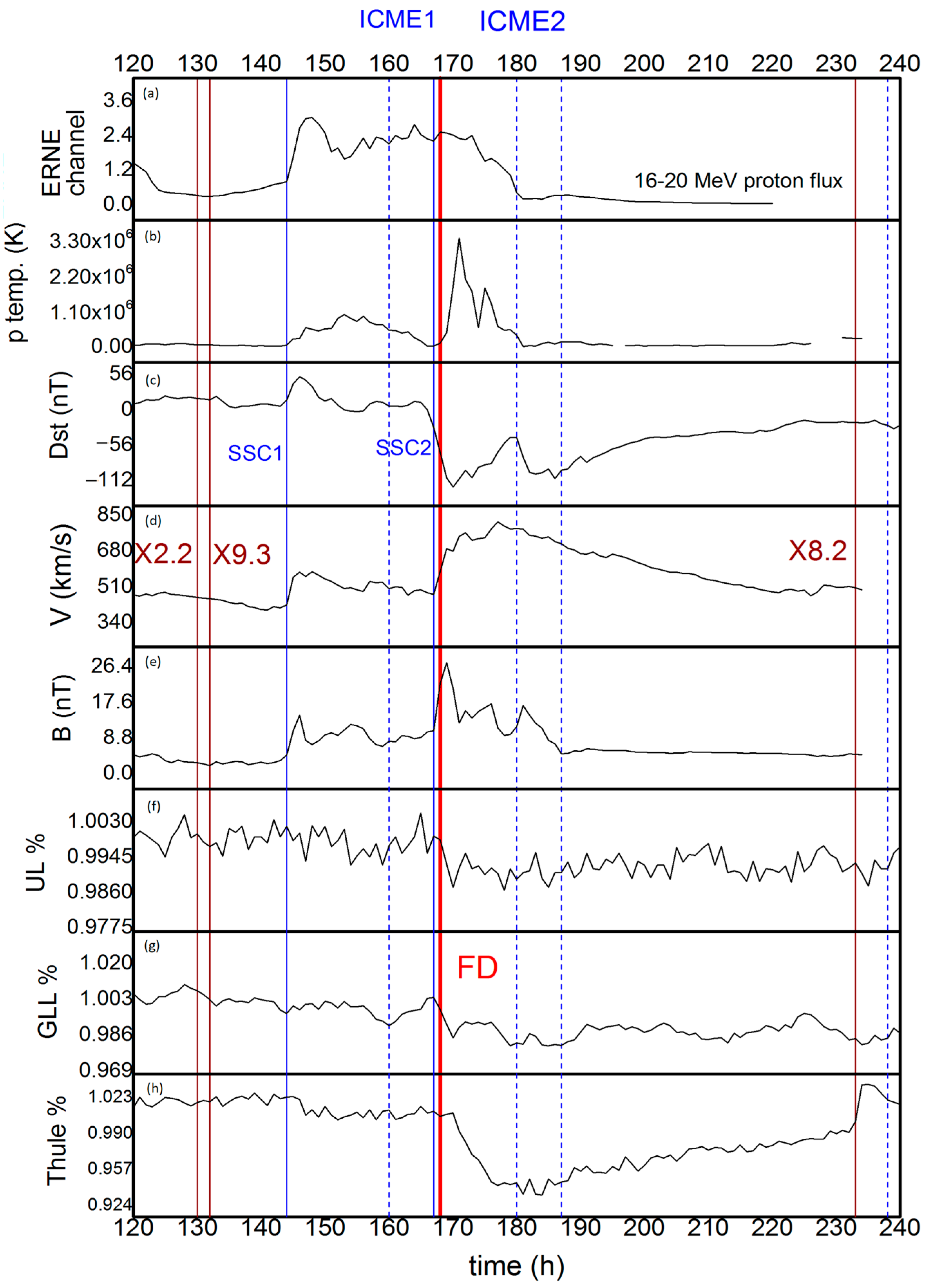
SEP fluence during strongly disturbed conditions of the heliosphere in early September 2017 was calculated from SOHO/ERNE data and modeled using double power law. Relationships between power exponents used to parameterize the shape of fluence spectrum and FD magnitude corrected for magnetospheric effect are consistent with ones expected for this type of event. Hourly time series of secondary CR flux, detected by several ground-based monitors and one shallow-underground monitor, show that all stations detected FD at the same time. Cross-correlation between these time series, and between CR time series and some geomagnetic activity indices, as well as selected IMF and solar wind parameters, are presented. Sensitivity of different stations to primary CR with different rigidity results in different time profiles, maximal decreases, and duration of recovery phase of FD;
-
We observed that a correlation between heliospheric and geomagnetic parameters decreases with increase of median energy of the CR detected by different stations and that shows an extension of CR modulation of complex CME-CME interaction structure initiated with strong SFs;
-
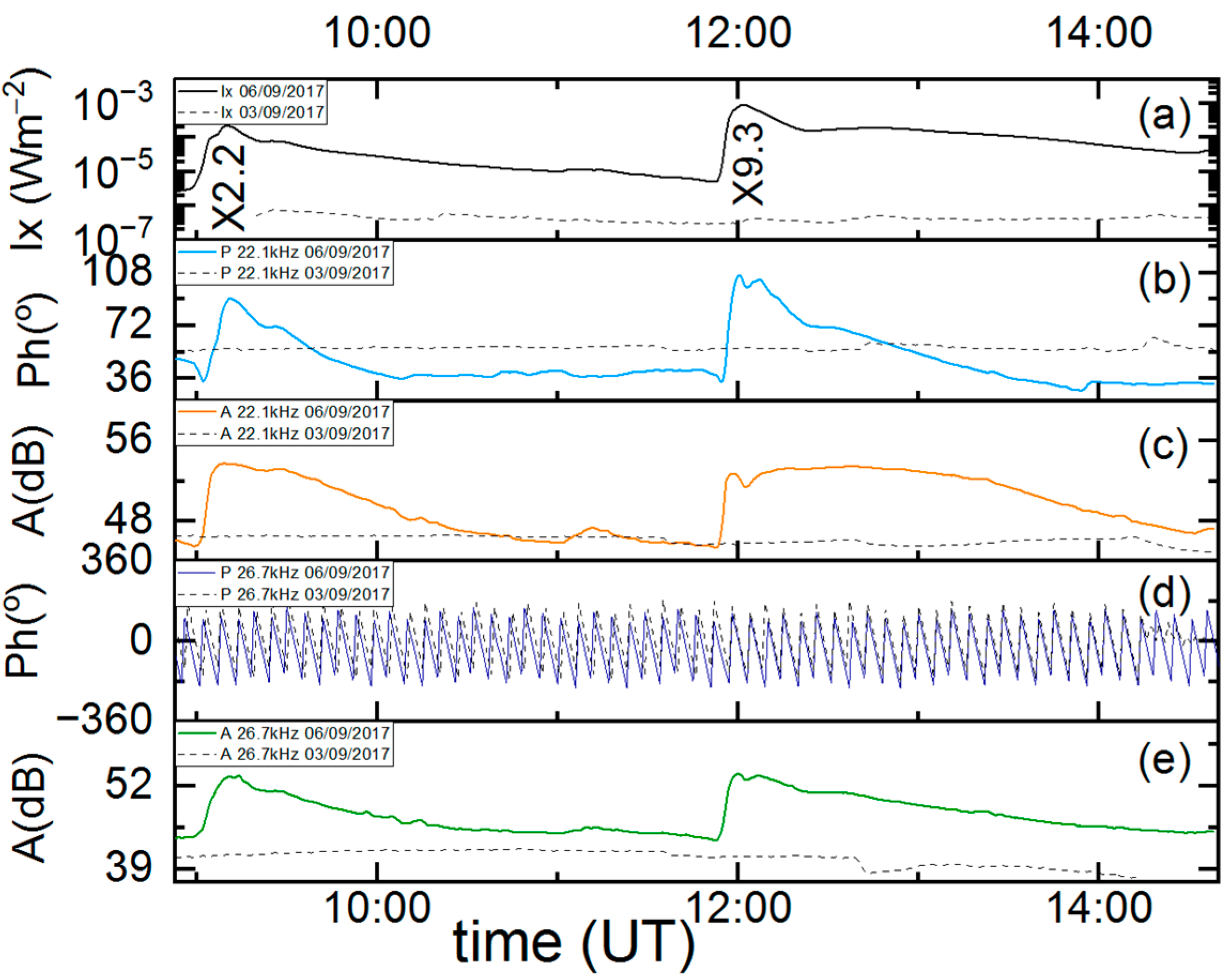
Impact of intense solar activity onto the Earth’s lower ionosphere, through analyzed X-class SFs, was clearly observed (perturbed amplitudes are 118% and 117% of unperturbed, while perturbed phases are 165% and 192% of unperturbed, for X2.2 and X9.3, respectively). BEL AbsPAL recordings of registered VLF signals during SF events are in correlation with X-ray flux (with time delays corresponding to the sluggishness of the ionosphere). Although X2.2 and X9.3 occurred back-to-back, it was possible to determine individual contributions of each SF based upon registered VLF signals;
-
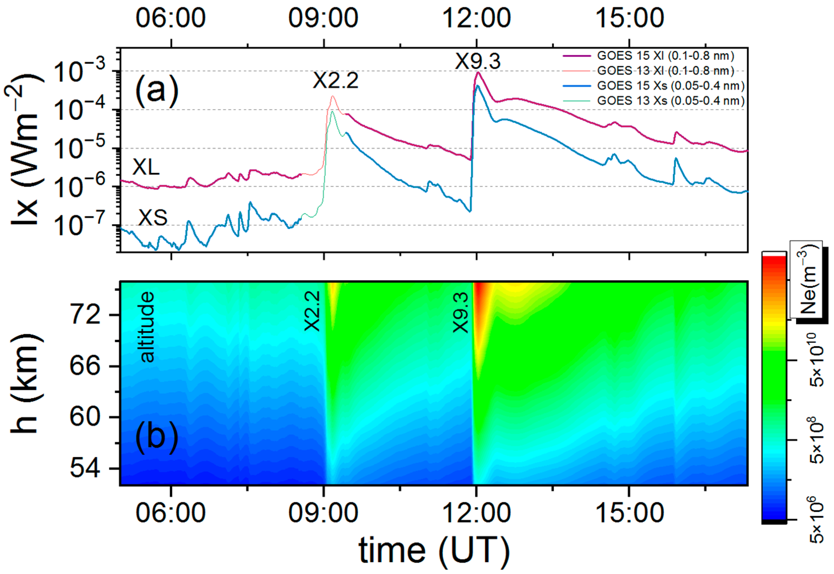
Numerical simulations were conducted through the application of the LWPC software package and the FlarED’ Method and Approximate Analytic Expression application’s novel approach. The ionospheric parameters (sharpness and effective reflection height) and electron density are in correlation with incident X-ray flux of soft range. Ne for these two SFs revealed the difference within one order of magnitude throughout the entire altitude range considered. Compared to quiet ionospheric conditions, Ne at the reference height increased by several orders of magnitude during both SF events. As monitored by BEL VLF station in the mid-latitudinal sector, both presented X-class SFs are common in properties and behavior, as could be expected for intense SF events, according to their strength. However, there is a significant difference in estimations of ionospheric parameters related to some other cases of reported X-class SFs from different sectors.
Although there are numerous papers related to the influence of SF events on Earth’s ionosphere, the vast majority of present case studies of selected SF events, more or less are extensively related to numbers of examined cases. X-class SF events have never been systematically studied in terms of lower ionospheric response. Coupling processes between such extreme space weather events and the lower ionosphere are not well understood. In addition, many intense SF events are related to other energetic solar events like CMEs and SEPs. Comprehensive research is needed especially in terms of retrieving a global (worldwide) lower ionospheric response to such strong events from propagation parameters of radio signals as a remote sensing technique. Case studies, although restricted to some selected events and with great contribution of “local” components contained within obtained and presented results, would provide substantial contributions.
This study emphasized the relevance of the ionospheric response, which was analyzed using a multi-instrument method, and gave a comprehensive examination of the events from the Sun to the Earth. It gave an insight into the sudden increase in ionization during the storm and strong SFs from the beginning of September 2017 and the potential effects on radio communication. Since conditions in the D-region of the ionosphere have a dramatic effect on high frequency communications and low frequency navigation systems, the ionospheric responses (and its parameters like β, H’ and Ne) to severe SFs are a key topic of study in ionospheric physics and are considered to be an important factor for space weather predictions, improvement of empirical models, and applications of machine learning techniques in atmospheric sciences.

Supplementary Materials

The following supporting information can be downloaded at: https://www.mdpi.com/article/10.3390/rs15051403/s1, Figure S1: Differential SEP fluxes during extreme solar event in September 2017, measured by SOHO/ERNE energetic particle sensors LET (Low Energy Detector) proton channels. Red vertical dashed lines indicate the time for the start and the end of interval used to calculate the integral flux.; Figure S2: Differential SEP fluxes during extreme solar event in September 2017, measured by SOHO/ERNE energetic particle sensors HET (High Energy Detector) proton channels. Red vertical dashed lines indicate the time for the start and the end of interval used to calculate the integral flux.; Figure S3: The geographic position of Belgrade (BEL) VLF receiver and the GQD transmitter (54.73°N, 2.88°W), Anthorn UK and TBB transmitter (37.43°N, 27.55°E) Bafa Turkey with GCP of sub-ionospheric propagating VLF signals.; Figure S4: Simultaneous variations of X-ray flux (red), phase (blue), and amplitude (orange) of GQD/22.10 kHz signal versus universal time UT during occurrence of X2.2 and X9.3 class solar flares of 6 September 2017 (from upper to lower panel). Observed amplitude and phase perturbations on GQD radio signal, as well as quiet signal (dashed black), are measured at Belgrade station. Time variation of soft X-ray irradiance is measured by GOES-15 satellite.; Figure S5: Lower ionospheric response to SF events of different strength across X-class (shaded gray area), obtained indirect modeling of VLF signals’ propagation parameters: (a) sharpness β (km−1), and (b) effective reflection height H’, (km) and (c) estimated corresponding electron densities Ne (m−3), in function of X-ray flux; results from our research are presented by black stars.; Figure S6: Magnitude of the FD versus the average CME velocity between the Sun and the Earth, calculated using the time of the beginning of the associated CME observations (a) Minimal Dst-index in the event, (b) maximal X-ray flare power (c) with associated flare indicated in red.

Author Contributions

Conceptualization, V.A.S.; writing—original draft preparation, V.A.S., A.K. and N.V.; writing—review and editing A.K., N.V., V.A.S., Z.M., M.S. and A.D. The authors had full access to the data and took responsibility for their integrity. All authors have read and agreed to the published version of the manuscript.

Funding

This work was funded by the Institute of Physics Belgrade, University of Belgrade, through a grant by the Ministry of Science, Technological Development and Innovations of the Republic of Serbia.

Data Availability Statement

VLF data were recorded at the Institute of Physics Belgrade, University of Belgrade and can be obtained upon request. Please contact V.A.S.

Acknowledgments

The article is based upon work from COST Action CA18212—Molecular Dynamics in the GAS phase (MD-GAS), supported by COST (European Cooperation in Science and Technology). Authors thank D. Šulić for instrumental set-up and useful discussions. OMNI data was made available by NASA/GSFC’s Space Physics Data Facility’s OMNIWeb service. This CME catalog is generated and maintained at the CDAW Data Center by NASA and The Catholic University of America in cooperation with the Naval Research Laboratory. SOHO is a project of international cooperation between ESA and NASA. We acknowledge the NMDB database, founded under the European Union’s FP7 program (contract no.213007) for providing data. We also gratefully acknowledge using data from the catalogue of Forbush effects and interplanetary disturbances provided by Cosmic Ray Group at the IZMIRAN Space Weather Prediction Center at Pushkov Institute of Terrestrial Magnetism, Ionosphere, and Radio Wave Propagation of the Russian Academy of Sciences.

Conflicts of Interest

The authors declare no conflict of interest. The funders had no role in the design of the study; in the collection, analyses, or interpretation of data; in the writing of the manuscript, or in the decision to publish the results.

References

  1. Manju, G.; Pant, T.K.; Devasia, C.V.; Ravindran, S.; Sridharan, R. Electrodynamical response of the Indian low-mid latitude ionosphere to the very large solar flare of 28 October 2003—A case study. Ann. Geophys. 2009, 27, 3853–3860. [Google Scholar] [CrossRef]
  2. Fu, H.; Zheng, Y.; Ye, Y.; Feng, X.; Liu, C.; Ma, H. Joint Geoeffectiveness and Arrival Time Prediction of CMEs by a Unified Deep Learning Framework. Remote Sens. 2021, 13, 1738. [Google Scholar] [CrossRef]
  3. Sahai, Y.; Becker-Guedes, F.; Fagundes, P.R.; Lima, W.L.C.; de Abreu, A.J.; Guarnieri, F.L.; Candido, C.M.N.; Pillat, V.G. Unusual ionospheric effects observed during the intense 28 October 2003 solar flare in the Brazilian sector. Ann. Geophys. 2007, 25, 2497–2502. [Google Scholar] [CrossRef]
  4. Le, H.; Liu, L.; Chen, Y.; Wan, W. Statistical analysis of ionospheric responses to solar flares in the solar cycle 23. J. Geophys. Res. Space Phys. 2013, 118, 576–582. [Google Scholar] [CrossRef]
  5. Srećković, V.A.; Šulić, D.M.; Ignjatović, L.; Vujčić, V. Low Ionosphere under Influence of Strong Solar Radiation: Diagnostics and Modeling. Appl. Sci. 2021, 11, 7194. [Google Scholar] [CrossRef]
  6. Kelley, M.C. The Earth’s Ionosphere: Plasma Physics and Electrodynamics; Academic Press: Cambridge, MA, USA, 2009. [Google Scholar]
  7. Barta, V.; Natras, R.; Srećković, V.; Koronczay, D.; Schmidt, M.; Šulic, D. Multi-instrumental investigation of the solar flares impact on the ionosphere on 05–06 December 2006. Front. Environ. Sci. 2022, 10, 904335. [Google Scholar] [CrossRef]
  8. Kolarski, A.; Srećković, V.A.; Mijić, Z.R. Response of the Earths Lower Ionosphere to Solar Flares and Lightning-Induced Electron Precipitation Events by Analysis of VLF Signals: Similarities and Differences. Appl. Sci. 2022, 12, 582. [Google Scholar] [CrossRef]
  9. Nina, A. Modelling of the Electron Density and Total Electron Content in the Quiet and Solar X-ray Flare Perturbed Ionospheric D-Region Based on Remote Sensing by VLF/LF Signals. Remote Sens. 2022, 14, 54. [Google Scholar] [CrossRef]
  10. Berdermann, J.; Kriegel, M.; Banyś, D.; Heymann, F.; Hoque, M.M.; Wilken, V.; Borries, C.; Heßelbarth, A.; Jakowski, N. Ionospheric Response to the X9.3 Flare on 6 September 2017 and Its Implication for Navigation Services Over Europe. Space Weather 2018, 16, 1604–1615. [Google Scholar] [CrossRef] [Green Version]
  11. Yasyukevich, Y.; Astafyeva, E.; Padokhin, A.; Ivanova, V.; Syrovatskii, S.; Podlesnyi, A. The 6 September 2017 X-Class Solar Flares and Their Impacts on the Ionosphere, GNSS, and HF Radio Wave Propagation. Space Weather 2018, 16, 1013–1027. [Google Scholar] [CrossRef]
  12. De Paula, V.; Segarra, A.; Altadill, D.; Curto, J.J.; Blanch, E. Detection of Solar Flares from the Analysis of Signal-to-Noise Ratio Recorded by Digisonde at Mid-Latitudes. Remote Sens. 2022, 14, 1898. [Google Scholar] [CrossRef]
  13. Demyanov, V.V.; Yasyukevich, Y.V.; Ishin, A.B.; Astafyeva, E.I. Ionospheric super-bubble effects on the GPS positioning relative to the orientation of signal path and geomagnetic field direction. GPS Solut. 2012, 16, 181–189. [Google Scholar] [CrossRef]
  14. Yashiro, S.; Gopalswamy, N. Statistical relationship between solar flares and coronal mass ejections. Proc. Int. Astron. Union 2008, 4, 233–243. [Google Scholar] [CrossRef] [Green Version]
  15. Desai, M.; Giacalone, J. Large gradual solar energetic particle events. Living Rev. Sol. Phys. 2016, 13, 3. [Google Scholar] [CrossRef] [Green Version]
  16. Freiherr von Forstner, J.L.; Guo, J.; Wimmer-Schweingruber, R.F.; Dumbović, M.; Janvier, M.; Démoulin, P.; Veronig, A.; Temmer, M.; Papaioannou, A.; Dasso, S.; et al. Comparing the Properties of ICME-Induced Forbush Decreases at Earth and Mars. J. Geophys. Res. Space Phys. 2020, 125, e2019JA027662. [Google Scholar] [CrossRef]
  17. Cane, H.V. Coronal Mass Ejections and Forbush Decreases. Space Sci. Rev. 2000, 93, 55–77. [Google Scholar] [CrossRef]
  18. Belov, A.V.; Eroshenko, E.A.; Oleneva, V.A.; Struminsky, A.B.; Yanke, V.G. What determines the magnitude of forbush decreases? Adv. Space Res. 2001, 27, 625–630. [Google Scholar] [CrossRef]
  19. Papaioannou, A.; Belov, A.; Abunina, M.; Eroshenko, E.; Abunin, A.; Anastasiadis, A.; Patsourakos, S.; Mavromichalaki, H. Interplanetary Coronal Mass Ejections as the Driver of Non-recurrent Forbush Decreases. Astrophys. J. 2020, 890, 101. [Google Scholar] [CrossRef]
  20. Belov, A.; Shlyk, N.; Abunina, M.; Belova, E.; Abunin, A.; Papaioannou, A. Solar Energetic Particle Events and Forbush Decreases Driven by the Same Solar Sources. Universe 2022, 8, 403. [Google Scholar] [CrossRef]
  21. Riley, P.; Love, J.J. Extreme geomagnetic storms: Probabilistic forecasts and their uncertainties. Space Weather 2017, 15, 53–64. [Google Scholar] [CrossRef]
  22. Eastwood, J.P.; Biffis, E.; Hapgood, M.A.; Green, L.; Bisi, M.M.; Bentley, R.D.; Wicks, R.; McKinnell, L.A.; Gibbs, M.; Burnett, C. The Economic Impact of Space Weather: Where Do We Stand? Risk Anal. 2017, 37, 206–218. [Google Scholar] [CrossRef] [PubMed] [Green Version]
  23. Kumar, A.; Kashyap, Y.; Kosmopoulos, P. Enhancing Solar Energy Forecast Using Multi-Column Convolutional Neural Network and Multipoint Time Series Approach. Remote Sens. 2023, 15, 107. [Google Scholar] [CrossRef]
  24. Alabdulgader, A.; McCraty, R.; Atkinson, M.; Dobyns, Y.; Vainoras, A.; Ragulskis, M.; Stolc, V. Long-Term Study of Heart Rate Variability Responses to Changes in the Solar and Geomagnetic Environment. Sci. Rep. 2018, 8, 2663. [Google Scholar] [CrossRef] [PubMed] [Green Version]
  25. Bruno, A.; Christian, E.R.; de Nolfo, G.A.; Richardson, I.G.; Ryan, J.M. Spectral Analysis of the September 2017 Solar Energetic Particle Events. Space Weather 2019, 17, 419–437. [Google Scholar] [CrossRef] [Green Version]
  26. Chamberlin, P.C.; Woods, T.N.; Didkovsky, L.; Eparvier, F.G.; Jones, A.R.; Machol, J.L.; Mason, J.P.; Snow, M.; Thiemann, E.M.B.; Viereck, R.A.; et al. Solar Ultraviolet Irradiance Observations of the Solar Flares During the Intense September 2017 Storm Period. Space Weather 2018, 16, 1470–1487. [Google Scholar] [CrossRef]
  27. Pikulina, P.; Mironova, I.; Rozanov, E.; Karagodin, A. September 2017 Solar Flares Effect on the Middle Atmosphere. Remote Sens. 2022, 14, 2560. [Google Scholar] [CrossRef]
  28. Vankadara, R.K.; Panda, S.K.; Amory-Mazaudier, C.; Fleury, R.; Devanaboyina, V.R.; Pant, T.K.; Jamjareegulgarn, P.; Haq, M.A.; Okoh, D.; Seemala, G.K. Signatures of Equatorial Plasma Bubbles and Ionospheric Scintillations from Magnetometer and GNSS Observations in the Indian Longitudes during the Space Weather Events of Early September 2017. Remote Sens. 2022, 14, 652. [Google Scholar] [CrossRef]
  29. Amaechi, P.O.; Akala, A.O.; Oyedokun, J.O.; Simi, K.G.; Aghogho, O.; Oyeyemi, E.O. Multi-Instrument Investigation of the Impact of the Space Weather Events of 6–10 September 2017. Space Weather 2021, 19, e2021SW002806. [Google Scholar] [CrossRef]
  30. Curto, J.J.; Marsal, S.; Blanch, E.; Altadill, D. Analysis of the Solar Flare Effects of 6 September 2017 in the Ionosphere and in the Earth’s Magnetic Field Using Spherical Elementary Current Systems. Space Weather 2018, 16, 1709–1720. [Google Scholar] [CrossRef] [Green Version]
  31. Bilitza, D. IRI the International Standard for the Ionosphere. Adv. Radio Sci. 2018, 16, 1–11. [Google Scholar] [CrossRef] [Green Version]
  32. Moraal, H. Cosmic-Ray Modulation Equations. Space Sci. Rev. 2013, 176, 299–319. [Google Scholar] [CrossRef]
  33. Dorman, L.I. Cosmic Rays in the Earth’s Atmosphere and Underground; Springer: Dordrecht, The Netherlands, 2004; Volume 303, p. 862. [Google Scholar]
  34. Zhang, J.L.; Tan, Y.H.; Wang, H.; Lu, H.; Meng, X.C.; Muraki, Y. The Yangbajing Muon–Neutron Telescope. In Nuclear Instruments and Methods in Physics Research Section A: Accelerators, Spectrometers, Detectors and Associated Equipment; Elsevier: Amsterdam, The Netherlands, 2010; Volume 623, pp. 1030–1034. [Google Scholar] [CrossRef]
  35. Veselinović, N.; Dragić, A.; Savić, M.; Maletić, D.; Joković, D.; Banjanac, R.; Udovičić, V. An underground laboratory as a facility for studies of cosmic-ray solar modulation. In Nuclear Instruments and Methods in Physics Research Section A: Accelerators, Spectrometers, Detectors and Associated Equipment; Elsevier: Amsterdam, The Netherlands, 2017; Volume 875, pp. 10–15. [Google Scholar]
  36. Savić, M.; Maletić, D.; Dragić, A.; Veselinović, N.; Joković, D.; Banjanac, R.; Udovičić, V.; Knežević, D. Modeling Meteorological Effects on Cosmic Ray Muons Utilizing Multivariate Analysis. Space Weather 2021, 19, e2020SW002712. [Google Scholar] [CrossRef]
  37. Ferguson, J. Computer Programs for Assessment of Long-Wavelength Radio Communications, Version 2.0: User’s Guide and Source Files; Space and Naval Warfare Systems Center: San Diego, CA, USA, 1998. [Google Scholar]
  38. Mitra, A.P. Lonospheric Effects of Solar Flares; Springer: Berlin/Heidelberg, The Netherlands, 1974; Volume 46. [Google Scholar]
  39. Wait, J.R.; Spies, K.P. Characteristics of the Earth-Ionosphere Waveguide for VLF Radio Waves; US Department of Commerce, National Bureau of Standards: Gaithersburg, MD, USA, 1964; Volume 13.
  40. Srećković, V.A.; Šulić, D.M.; Vujčić, V.; Mijić, Z.R.; Ignjatović, L.M. Novel Modelling Approach for Obtaining the Parameters of Low Ionosphere under Extreme Radiation in X-Spectral Range. Appl. Sci. 2021, 11, 11574. [Google Scholar] [CrossRef]
  41. AR12673 History. Available online: http://helio.mssl.ucl.ac.uk/helio-vo/solar_activity/arstats/arstats_page4.php?region=12673 (accessed on 14 December 2022).
  42. Space Weather Prediction Center (IZMIRAN). Available online: http://spaceweather.izmiran.ru/eng/dbs.html (accessed on 22 January 2022).
  43. Wold, A.M.; Mays, M.L.; Taktakishvili, A.; Jian, L.K.; Odstrcil, D.; MacNeice, P. Verification of real-time WSA−ENLIL+Cone simulations of CME arrival-time at the CCMC from 2010 to 2016. J. Space Weather Space Clim. 2018, 8, A17. [Google Scholar] [CrossRef] [Green Version]
  44. Gopalswamy, N.; Yashiro, S.; Michalek, G.; Stenborg, G.; Vourlidas, A.; Freeland, S.; Howard, R. The SOHO/LASCO CME Catalog. Earth Moon Planets 2009, 104, 295–313. [Google Scholar] [CrossRef]
  45. Werner, A.L.E.; Yordanova, E.; Dimmock, A.P.; Temmer, M. Modeling the Multiple CME Interaction Event on 6–9 September 2017 with WSA-ENLIL+Cone. Space Weather 2019, 17, 357–369. [Google Scholar] [CrossRef]
  46. SPDF - OMNIWeb Service. Available online: https://spdf.gsfc.nasa.gov/pub/data/omni/low_res_omni/ (accessed on 10 November 2022).
  47. Torsti, J.; Valtonen, E.; Lumme, M.; Peltonen, P.; Eronen, T.; Louhola, M.; Riihonen, E.; Schultz, G.; Teittinen, M.; Ahola, K.; et al. Energetic particle experiment ERNE. Sol. Phys. 1995, 162, 505–531. [Google Scholar] [CrossRef]
  48. Multi-Source Spectral Plots (MSSP) of Energetic Particle. Available online: https://omniweb.gsfc.nasa.gov/ftpbrowser/flux_spectr_m.html (accessed on 25 October 2022).
  49. Savić, M.; Veselinović, N.; Dragić, A.; Maletić, D.; Joković, D.; Udovičić, V.; Banjanac, R.; Knežević, D. New insights from cross-correlation studies between solar activity indices and cosmic-ray flux during Forbush decrease events. Adv. Space Res. 2022, 71, 2006–2016. [Google Scholar] [CrossRef]
  50. Band, D.; Matteson, J.; Ford, L.; Schaefer, B.; Palmer, D.; Teegarden, B.; Cline, T.; Briggs, M.; Paciesas, W.; Pendleton, G.; et al. BATSE Observations of Gamma-Ray Burst Spectra. I. Spectral Diversity. Astrophys. J. 1993, 413, 281. [Google Scholar] [CrossRef]
  51. Ellison, D.C.; Ramaty, R. Shock acceleration of electrons and ions in solar flares. Astrophys. J. 1985, 298, 400–408. [Google Scholar] [CrossRef]
  52. Mottl, D.A.; Nymmik, R.A.; Sladkova, A.I. Energy spectra of high-energy SEP event protons derived from statistical analysis of experimental data on a large set of events. AIP Conf. Proc. 2001, 552, 1191–1196. [Google Scholar] [CrossRef]
  53. Zhao, L.; Zhang, M.; Rassoul, H.K. Double power laws in the event-integrated solar energetic particle spectrum. Astrophys. J. 2016, 821, 62. [Google Scholar] [CrossRef] [Green Version]
  54. Miteva, R.; Samwel, S.W.; Zabunov, S.; Dechev, M. On the flux saturation of SOHO/ERNE proton events. Bulg. Astron. J. 2020, 33, 99. [Google Scholar]
  55. NOAA National Centers for Environmental Information. Available online: https://satdat.ngdc.noaa.gov/sem/goes/data/avg/ (accessed on 10 October 2022).
  56. Žigman, V.; Grubor, D.; Šulić, D. D-region electron density evaluated from VLF amplitude time delay during X-ray solar flares. J. Atmos. Sol.-Terr. Phys. 2007, 69, 775–792. [Google Scholar] [CrossRef]
  57. Kolarski, A.; Grubor, D. Sensing the Earth’s low ionosphere during solar flares using VLF signals and goes solar X-ray data. Adv. Space Res. 2014, 53, 1595–1602. [Google Scholar] [CrossRef] [Green Version]
  58. Kolarski, A.; Srećković, V.A.; Mijić, Z.R. Monitoring solar activity during 23/24 solar cycle minimum through VLF radio signals. Contrib. Astron. Obs. Skaln. Pleso 2022, 52, 105. [Google Scholar] [CrossRef]
  59. Šulić, D.; Srećković, V.A.; Mihajlov, A.A. A study of VLF signals variations associated with the changes of ionization level in the D-region in consequence of solar conditions. Adv. Space Res. 2016, 57, 1029–1043. [Google Scholar] [CrossRef] [Green Version]
  60. Dorman, L.; Tassev, Y.; Velinov, P.I.Y.; Mishev, A.; Tomova, D.; Mateev, L. Investigation of exceptional solar activity in September 2017: GLE 72 and unusual Forbush decrease in GCR. J. Phys. Conf. Ser. 2019, 1181, 012070. [Google Scholar] [CrossRef]
  61. Neutron Monitor Database. Available online: https://www.nmdb.eu/ (accessed on 20 October 2022).
  62. Kojima, H.; Shibata, S.; Oshima, A.; Hayashi, Y.; Antia, H.; Dugad, S.; Fujii, T.; Gupta, S.K.; Kawakami, S.; Minamino, M.; et al. Rigidity Dependence of Forbush Decreases. In Proceedings of the 33rd International Cosmic Ray Conference, Rio de Janeiro, Brazil, 2–9 July 2013. [Google Scholar]
  63. Near-Earth Interplanetary Coronal Mass Ejections Since January 1996. Available online: https://izw1.caltech.edu/ACE/ASC/DATA/level3/icmetable2.htm (accessed on 15 October 2022).
  64. Soho Lasco Cme Catalog Cdaw Data Center. Available online: https://cdaw.gsfc.nasa.gov/CME_list/ (accessed on 10 November 2022).
  65. Scolini, C.; Chané, E.; Temmer, M.; Kilpua, E.K.J.; Dissauer, K.; Veronig, A.M.; Palmerio, E.; Pomoell, J.; Dumbović, M.; Guo, J.; et al. CME–CME Interactions as Sources of CME Geoeffectiveness: The Formation of the Complex Ejecta and Intense Geomagnetic Storm in 2017 Early September. Astrophys. J. Suppl. Ser. 2020, 247, 21. [Google Scholar] [CrossRef]
  66. Badruddin, B.; Aslam, O.P.M.; Derouich, M.; Asiri, H.; Kudela, K. Forbush Decreases and Geomagnetic Storms During a Highly Disturbed Solar and Interplanetary Period, 4–10 September 2017. Space Weather 2019, 17, 487–496. [Google Scholar] [CrossRef]
  67. Miteva, R.; Klein, K.L.; Malandraki, O.; Dorrian, G. Solar Energetic Particle Events in the 23rd Solar Cycle: Interplanetary Magnetic Field Configuration and Statistical Relationship with Flares and CMEs. Sol. Phys. 2013, 282, 579–613. [Google Scholar] [CrossRef] [Green Version]
  68. Ravishankar, A.; Michałek, G. Non-interacting coronal mass ejections and solar energetic particles near the quadrature configuration of Solar TErrestrial RElations Observatory. Astron. Astrophys. 2020, 638, A42. [Google Scholar] [CrossRef]
  69. Pandey, U.; Singh, B.; Singh, O.P.; Saraswat, V.K. Solar flare induced ionospheric D-region perturbation as observed at a low latitude station Agra, India. Astrophys. Space Sci. 2015, 357, 35. [Google Scholar] [CrossRef]
  70. Gavrilov, B.G.; Ermak, V.M.; Lyakhov, A.N.; Poklad, Y.V.; Rybakov, V.A.; Ryakhovsky, I.A. Reconstruction of the Parameters of the Lower Midlatitude Ionosphere in M- and X-Class Solar Flares. Geomagn. Aeron. 2020, 60, 747–753. [Google Scholar] [CrossRef]
  71. Venkatesham, K.; Singh, R. Extreme space-weather effect on D-region ionosphere in Indian low latitude region. Curr. Sci. 2018, 114, 1923–1926. [Google Scholar] [CrossRef]
  72. Thomson, N.R.; Rodger, C.J.; Clilverd, M.A. Large solar flares and their ionospheric D region enhancements. J. Geophys. Res. Space Phys. 2005, 110. [Google Scholar] [CrossRef] [Green Version]
  73. Grubor, D.; Šulić, D.; Žigman, V. The response of the Earth-ionosphere VLF waveguide to the January 15-22 2005 solar events. In Proceedings of the IUGG XXIV General Assembly, Perugia, Italy, 2–13 July 2007. [Google Scholar]
  74. Kolarski, A.; Grubor, D. Monitoring VLF signal perturbations induced by solar activity during January 2005. In Proceedings of the The XIX Serbian Astronomical Conference, Belgrade, Serbia, 13–17 October 2020; pp. 387–390. [Google Scholar]
  75. Kumar, S.; Kumar, A.; Menk, F.; Maurya, A.K.; Singh, R.; Veenadhari, B. Response of the low-latitude D region ionosphere to extreme space weather event of 14–16 December 2006. J. Geophys. Res. Space Phys. 2015, 120, 788–799. [Google Scholar] [CrossRef] [Green Version]
  76. Tan, L.M.; Thu, N.N.; Ha, T.Q.; Marbouti, M. Study of solar flare induced D-region ionosphere changes using VLF amplitude observations at a low latitude site. Indian J. Radio Space Phys. 2014, 43, 197–246. [Google Scholar]
  77. McRae, W.M.; Thomson, N.R. Solar flare induced ionospheric D-region enhancements from VLF phase and amplitude observations. J. Atmos. Sol.-Terr. Phys. 2004, 66, 77–87. [Google Scholar] [CrossRef]
  78. Zhao, L.L.; Zhang, H. Transient galactic cosmic-ray modulation during solar cycle 24: A comparative study of two prominent forbush decrease events. Astrophys. J. 2016, 827, 13. [Google Scholar] [CrossRef]
  79. Lingri, D.; Mavromichalaki, H.; Belov, A.; Eroshenko, E.; Yanke, V.; Abunin, A.; Abunina, M. Solar Activity Parameters and Associated Forbush Decreases During the Minimum between Cycles 23 and 24 and the Ascending Phase of Cycle 24. Sol. Phys. 2016, 291, 1025–1041. [Google Scholar] [CrossRef]
Figure 1. Hourly time series (UT) for several different proton channels from SOHO/ERNE ((a) 1.3–1.6 MeV, (b) 10–13 MeV, (c) 20–25 MeV, (d) 40–50 MeV channels’ energy bands) for September 2017. Integration interval for spectral fluence is indicated with red vertical dashed lines.
Remotesensing 15 01403 g001
Figure 2. Fluence spectrum for energetic protons measured by SOHO/ERNE at L1 during FD in September 2017. Data points represent fluence integrated in different energy channels over time of duration of the event, while red line represents the fitted double power law.
Remotesensing 15 01403 g002
Figure 3. Simultaneous variations of X-ray flux (a) with phase delay, (b) amplitude delay, (c) variations of GQD/22.10 kHz and phase delay, (d) amplitude delay, (e) variations of TBB/26.70 kHz signals versus universal time UT during occurrence of X2.2 and X9.3 class SFs of 6 September 2017. Observed amplitude and phase perturbations with the quiet signal of 3 September 2017 (dashed black) are measured at Belgrade station. Time variation of soft X-ray irradiance is measured by GOES-15 satellite.
Remotesensing 15 01403 g003
Figure 4. Simultaneous variations of the effective reflection height h’, (a) sharpness β, (b) and X-ray flux (c) during the occurrence of two successive X-ray flares of 6 September 2017.
Remotesensing 15 01403 g004
Figure 5. The height profile of electron density at peak time for two successive X-class SFs of 6 September 2017.
Remotesensing 15 01403 g005
Figure 6. Variation of X-ray flux (a) as measured by GOES-15 and -13 satellites and the surface plot of corresponding electron density profile (b) versus universal time UT during two successive X-class SFs of 6 September 2017. The results are obtained using simple approximative Equation (3).
Remotesensing 15 01403 g006
Figure 7. Normalized time series of secondary CR flux detected at several ground and one shallow-underground monitors: (a) ground (GLL) and (b) underground (UL) detector at Belgrade muon station, (c) South pole NM (SOPO), (d) Thule NM (THUL), and (e) Athens NM (ATHN).
Remotesensing 15 01403 g007
Figure 8. Hourly variation in CR intensity measured at ground station ((f) UL, (g) GLL, (h) Thule), (e) magnitude of interplanetary magnetic field B, (d) velocity of solar wind V, (c) Dst index, (b) proton temperature, and (a) one of the proton channels measured by ERNE/SOHO during early September 2017 (period 4th–10th).
Remotesensing 15 01403 g008
Table 1. VLF transmitting sites.
Freq.
(kHz)
CountryLatitude
(°)
Longitude
(°)
GCP
(km)
Prop. Path Direction
Transmitter:
GQD22.10UK54.73 N2.88 W1982NW to SE
TBB26.70Turkey37.43 N27.55 E1020SE to NW
Table 2. Statistical correlation between ground stations during September 2017.
Pearson Corr.ATHNSOPOGLLULTHUL
ATHN10.550840.434430.50560.61535
SOPO 10.189410.451940.81747
GLL 10.693250.36496
UL 10.51526
THUL 1
Table 3. Statistical correlation (with significance) between time series of CR flux measured at ground stations and selected space weather parameters during 5–10 September 2017.
Pearson Corr.Thule GLL UL
Thule1
GLL0.67213(<10−6)1
UL0.62741(<10−6)0.75552(<10−6)1
Average B−0.238(<0.008)−0.2420.007−0.243<0.007
SW speed−0.80562(<10−6)−0.62829(<10−6)−0.58503(<10−6)
Dst Index0.77923(<10−6)0.6979(<10−6)0.65494(<10−6)
Proton Channel 16–20 MeV0.43083<10−50.38276<10−40.31715<10−3
Disclaimer/Publisher’s Note: The statements, opinions and data contained in all publications are solely those of the individual author(s) and contributor(s) and not of MDPI and/or the editor(s). MDPI and/or the editor(s) disclaim responsibility for any injury to people or property resulting from any ideas, methods, instructions or products referred to in the content.

