A Semantic Segmentation Framework for Hyperspectral Imagery Based on Tucker Decomposition and 3DCNN Tested with Simulated Noisy Scenarios

Abstract

The present work, unlike others, does not try to reduce the noise in hyperspectral images to increase the semantic segmentation performance metrics; rather, we present a classification framework for noisy Hyperspectral Images (HSI), studying the classification performance metrics for different SNR levels and where the inputs are compressed. This framework consists of a 3D Convolutional Neural Network (3DCNN) that uses as input data a spectrally compressed version of the HSI, obtained from the Tucker Decomposition (TKD). The advantage of this classifier is the ability to handle spatial and spectral features from the core tensor, exploiting the spatial correlation of remotely sensed images of the earth surface. To test the performance of this framework, signal-independent thermal noise and signal-dependent photonic noise generators are implemented to simulate an extensive collection of tests, from 60 dB to −20 dB of Signal-to-Noise Ratio (SNR) over three datasets: Indian Pines (IP), University of Pavia (UP), and Salinas (SAL). For comparison purposes, we have included tests with Support Vector Machine (SVM), Random Forest (RF), 1DCNN, and 2DCNN. For the test cases, the datasets were compressed to only 40 tensor bands for a relative reconstruction error less than 1%. This framework allows us to classify the noisy data with better accuracy and significantly reduces the computational complexity of the Deep Learning (DL) model. The framework exhibits an excellent performance from 60 dB to 0 dB of SNR for 2DCNN and 3DCNN, achieving a Kappa coefficient from 0.90 to 1.0 in all the noisy data scenarios for a representative set of labeled samples of each class for training, from 5% to 10% for the datasets used in this work. The source code and log files of the experiments used for this paper are publicly available for research purposes.

1. Introduction

Hyperspectral imaging studies the interactions between observed scenes and the electromagnetic spectrum [1]. For example, it allows for measuring the amount of light reflected into a spectral sensor. From these measurements, it is possible to obtain a distinctive spectral signature composed of different wavelength channels [2]. If it is assigned a label corresponding to the ground truth, with the help of a human expert or a clustering algorithm, a Machine Learning classifier can be trained using supervised learning [2]. The hyperspectral image capturing process is far from ideal [3]; it is well known that every signal will be prone to being corrupted by different kinds of noise depending on the electronics’ quality, environment of capture, and many others factors. For example, hyperspectral sensors are mounted on airplanes, drones, or satellites causing the capture of data cubes to be highly expensive and noisy. Thus, the need for new methods that are robust to noisy environments for expanding the possible range of applications. To address this task, this work tests the performance of a 3DCNN for noisy hyperspectral images, which is a semantic segmentation algorithm based on the spatial–spectral feature extraction pixel-by-pixel. Given the high computational complexity of the 3DCNN with the original HSI, a dimensionality reduction method based on Tucker Decomposition compresses the spectral dimension of the input, independent of the low signal-to-noise ratio.

1.1. Related Work

It is usual to consider data denoising as a preprocessing step for classification. As is well known, there are many denoising algorithms for hyperspectral imagery [3,4,5,6,7,8,9], which aims to recover the clean signal from the noisy one. These algorithms are particularly useful when the posterior tasks analyze the spectral signature for qualitatively studies. On the other hand, the pixel-based semantic segmentation (classification) could be based on a wide range of algorithms, artificial neural networks architectures, or feature extraction techniques; for example, Convolutional Neural Networks (CNNs) have demonstrated outstanding results performing spatial and spectral feature extraction [2,10,11,12,13,14,15]. Semantic segmentation techniques for RGB images, such as transfer learning [16,17,18,19], have been applied to spectral imagery [20] in combination with fully convolutional models, such as the well-known U-net [21,22,23,24]. There are other techniques specifically designed for noise–robust classification, e.g., based on band fusion [25,26] or feature extraction as a pre-processing step for a classification algorithm [27,28,29,30,31]. In some applications of optical remote sensing satellites in orbit, using atmospheric correction as an example [32,33], for hyperspectral [34,35] earth surface monitoring missions, the first task is to perform semantic segmentation to obtain a classification mask, from which the atmospherically corrected image is estimated.

This framework aims to classify the noisy data pixel by pixel. For example, 3DCNN can extract spatial and spectral features despite the low Signal to Noise Ratio (SNR). However, there is a drawback of using these models caused by the computational complexity of having such huge datasets. Thus, we propose using Tucker Decomposition with a 3DCNN to combine and improve the properties of DL and Decomposition in a single noise robust framework. TKD shows excellent compression ratios with minimal or no effects in the segmentation performance of DL models given that it found a lower-rank representation of the original tensor, capturing the high spatial–spectral correlation of the data [36,37]. Not only that, in this work, we have shown that TKD helps to improve the classification performance where there are a representative number of samples of each class for training. Finally, in

Table 1. Main papers used for the proposed framework and its contribution.

	Author	Contribution
Tensor	Kolda and Bader [38]	Tensor theory
	López et al. [36]	Use of the TKD for semantic segmentation tasks
Noise	Bourennane et al. [4]	Noise theory and noise model
	Liu et al. [39]	Noise model and noise generation
	Rasti et al. [3]	Noise theory and classification test methodology
Classification	Paoletti et al. [2]	Classifiers code, architectures, and theory
	Chen et al. [10]	Spatial–Spectral feature extraction theory
	Li et al. [40]	3DCNN architecture
	Fu et al. [25]	Noisy-robust classification
Metrics	Grandini et al. [41]	Metrics used for multi-class classification evaluation
	Luque et al. [42]	Impact of class unbalance for classification performance metrics

, we have a summary of the major papers consulted for the proposed semantic segmentation framework.

1.2. Contributions

Our main contributions are three-fold:

• This work provides the remote sensing community with a framework based on a 3DCNN and Tucker Decomposition, performing semantic segmentation of noisy hyperspectral images, from an SNR of from 60 dB to 0 dB, outperforming other classical classifiers such as RF and SVM.
• Taking advantage of the spectral correlation of the data, we perform the Tucker Decomposition compressing only in the spectral domain; for example, for the three data sets studied to 40 new tensor bands and achieving a relative reconstruction error of less than 1%. This compression of the spectral domain of the input space reduces the computational complexity, consequently reducing the training time ratio by up to 29 times with respect to the original input space, depending on the case.
• TKD not only reduces the computational complexity but also increases the classification performance. This improvement was most significant for training set sizes on the order of from 5% to 3%. Furthermore, the behavior of TKD under different SNR are studied for the three used datasets.

The remainder of this work explains the basic concepts of tensor algebra, the noise model used, and the architecture of the DL model in Section 2. Section 3 describes the proposed framework. Section 4 analyzes the experiments. Finally, Section 5 and Section 6 present the discussion and conclusions, respectively.

2. Mathematical Background

This section presents a short description of the theoretical concepts used in each stage of the proposed semantic segmentation framework. First, tensor theory for HSI representation and compression based on the TKD is used [38]. Second, a noise model for hyperspectral imagery is used in this paper for noise generation [3,4,39]. Finally, DL spectral and spatial feature extraction models [2,10,40] with metrics are used to compare ground truth labels and predicted ones for unbalanced training scenarios [41,42,43].

2.1. Tensor Algebra

Nowadays, research in tensor data analysis is finding new novel properties and applications on spectral images [4,8,9,36,44,45,46,47,48]. For this reason, this section presents an overview of the tensors theory, and the representation of an HSI as a tensor.

For tensor algebra, the work of Kolda and Bader [38] is our main reference. Using its notation, a scalar is denoted by x, and the vectors and matrices are denoted by $\mathbf{x}$ and $\mathbf{X}$, respectively, which can also be seen as tensors. For example, a first-order tensor is a vector, and a second-order tensor is a matrix. A third- or higher-order tensor is denoted by $\mathcal{X}$ with elements $x_{i,j,...,n}$. Thus, naturally, a third-order tensor may be represented as a cube of elements. Besides, ${\mathbf{x}}_i$ is the $i^{th}$ column of a matrix $\mathbf{X}$, and ${\mathbf{a}}^{\left(n\right)},{\mathbf{A}}^{\left(n\right)}$ are the $n^{th}$ vector or matrix in a sequence of vectors or matrices, respectively. Now, a mode-n fiber is a vector obtained by fixing all indices, except the one corresponding to the $n^{th}$-dimension [38] (pp. 457–460). ${\mathbf{X}}_{\left(n\right)}$ is a mode-n matricization of an $N^{th}$-order tensor $\mathcal{X}$, where the mode-n fibers are arranged to be the matrix columns. Lastly, $\parallel \mathcal{X}\parallel$ denotes the tensor norm of $\mathcal{X}\in {\mathbb{R}}^{I_1\times I_2\times \dots \times I_N}$, as described by Equation (1); this is analogous to the matrix Frobenius norm.

$$\parallel \mathcal{X}\parallel =\sqrt{\sum _{i_1=1}^{I_1}\sum _{i_2=1}^{I_2}\dots \sum _{i_N=1}^{I_N}{x}_{i_1{i}_2\dots i_N}^2}.$$

(1)

An element of the new vector space generated by the outer product of the N vector spaces on the same field $\mathbb{R}$ is an $N^{th}$-order tensor $\mathcal{X}$. Thus, a tensor can be seen as a multi-dimensional array of N dimensions. The order of a tensor is also called the ways or modes [38]. An hyperspectral image $\mathcal{H}$ in Figure 1 can be represented as a third-order tensor $\mathcal{H}\in {\mathbb{R}}^{I_1\times I_2\times I_3}$, where $I_1$ and $I_2$ are image height and width, respectively. $I_3$ is the number of bands in which the electromagnetic spectrum is captured. Then, the element $x_{i_1,i_2,i_3}$ is the pixel value at position $(i_1,i_2)$ at band $i_3$.

In order to introduce the concept of TKD, the concepts of rank-one, vector outer product, n-$mode$ product, and n-rank are required. A rank-one tensor of the $N^{th}$-order $\mathcal{X}\in {\mathbb{R}}^{I_1\times I_2\times \dots \times I_N}$ can be represented as the outer product of vectors [38],

$$\mathcal{X}={\mathbf{a}}^{\left(1\right)}\circ {\mathbf{a}}^{\left(2\right)}\circ \dots \circ {\mathbf{a}}^{\left(N\right)},$$

(2)

where the symbol “∘”, at Equation (2), represents the vector outer product. Thus, each element $x_{i_1,i_2,...,i_n}$ of $\mathcal{X}$ is obtained from the corresponding vector elements [38]:

$$x_{i_1,i_2,...,i_n}=a_{i_1}^{\left(1\right)}{a}_{i_2}^{\left(2\right)}\dots a_{i_N}^{\left(N\right)}\mathrm{for}\mathrm{all}1\le i_n\le I_n.$$

(3)

The n-rank, ${\mathrm{rank}}_n\left(\mathcal{X}\right)$, is the column rank of the matrix ${\mathbf{X}}_{\left(n\right)}$. For easy-reading reasons, it is defined ${\mathrm{rank}}_n\left(\mathcal{X}\right)$ as $R_n$ of $\mathcal{X}$ for $n=1,...,N$. For an HSI represented as a third-order tensor, $\mathcal{H}\in {\mathbb{R}}^{I_1\times I_2\times I_3}$, ${\mathrm{rank}}_1\left(\mathcal{H}\right)$, and ${\mathrm{rank}}_2\left(\mathcal{H}\right)$ correspond to the spatial domain of the image, such that $1\le {\mathrm{rank}}_1\left(\mathcal{H}\right)\le I_1$ and $1\le {\mathrm{rank}}_2\left(\mathcal{H}\right)\le I_2$. In the same way, ${\mathrm{rank}}_3\left(\mathcal{H}\right)$ and $1\le {\mathrm{rank}}_3\left(\mathcal{H}\right)\le I_3$ corresponds to the spectral domain. Finally, for the n-mode product of a tensor with a matrix, $\mathcal{X}{\times }_n\mathbf{U}$, with $\mathbf{U}\in {\mathbb{R}}^{J\times I_n}$, the resultant tensor will have dimensions $I_1\times \dots \times I_{n-1}\times J\times I_{n+1}\times \dots \times I_N$ [38] (pp. 460–461):

$${\left(\mathcal{X}{\times }_n\mathbf{U}\right)}_{i_1\dots i_{n-1}j{i}_{n+1}\dots i_N}=\sum _{i_n=1}^{I_n}{x}_{i_1{i}_2\dots i_N}{u}_{j{i}_n}.$$

(4)

Tucker in 1966 introduced the now-called Tucker Decomposition [50]. It is a form of higher-order PCA and there are several tensor decompositions derived from this one. The Tucker Decomposition (TKD) decomposes a tensor of $N^{th}$-order into a core tensor of the same order but could have different dimensions, multiplied by a transformation matrix along each mode [38]. The Tucker Decomposition for a third-order tensor, e.g., see Figure 2, for an HSI representation, $\mathcal{X}\in {\mathbb{R}}^{I\times J\times K}$, is defined as:

$$\mathcal{X}\approx \mathcal{G}{\times }_1\mathbf{A}{\times }_2{\mathbf{B}\times }_3\mathbf{C}=\sum _{p=1}^P\sum _{q=1}^Q\sum _{r=1}^R{g}_{pqr}{\mathbf{a}}_p\circ {\mathbf{b}}_q\circ {\mathbf{c}}_r=\left[\left[\mathcal{G};\mathbf{A},\mathbf{B},\mathbf{C}\right]\right],$$

(5)

where $P\le I$, $Q\le J$ and $R\le K$.

Element-wise, the Tucker Decomposition in Equation (5) is provided by:

$$x_{ijk}\approx \sum _{p=1}^P\sum _{q=1}^Q\sum _{r=1}^R{g}_{pqr}{a}_{ip}{b}_{jq}{c}_{kr}fori=1,...,I,j=1,...,J,k=1,...,K.$$

(6)

The entries of the core tensor $\mathcal{G}\in {\mathbb{R}}^{P\times Q\times R}$ “show the level of interaction between the different components”. P, Q, and R are the new dimensions of the factor matrices $\mathbf{A}$, $\mathbf{B}$, and $\mathbf{C}$, respectively, which can be seen as the principal components in each mode. “If P, Q, R are smaller than I,J,K, the core tensor $\mathcal{G}$ is a compressed version of $\mathcal{X}$”.

According with Kolda and Bader [38], for $R_n={\mathrm{rank}}_n\left(\mathcal{X}\right)$, an exact Tucker Decomposition of rank $\left(R_1,R_2,...,R_N\right)$ can be computed. Another case is “the truncated Tucker Decomposition of rank $\left(R_1,R_2,...,R_N\right)$, when $R_n<{\mathrm{rank}}_n\left(\mathcal{X}\right)$ for one or more n, then it will be necessarily inexact and more difficult to compute.” Tucker Decomposition can compress along selected dimensions. To do this, we use the Tucker1 Decomposition, defined in [38], which fixes two factor matrices to be the identity matrix,

$$\mathcal{X}\approx \mathcal{G}{\times }_1\mathbf{A}=\left[\left[\mathcal{G};\mathbf{A},\mathbf{I},\mathbf{I}\right]\right].$$

(7)

2.2. Noise Model

Noise is intrinsic to any signal and hyperspectral imaging is not an exception. There are many sources and kinds of noise present on HSIs mentioned in this section. In general, the noise can be distinguished into two classes [4]: the fixed pattern noise and the random noise. The first one is due to calibration errors, and it is not of interest in this work. Instead, random noise, due to its stochastic nature, can be studied and generated from a suitable noise model. For new-generation imaging spectrometers used in hyperspectral imagery, the random noise mainly comes from two aspects: Signal-Dependent (SD) photonic noise and Signal-Independent (SI) electronic noise, also known as thermal (Johnson) noise [51].

Although, the noise model used in this paper is due to the work of Bourennane et al. [4], we are not addressing the signal denoising process; rather, we use it for the simulation of the noisy data scenarios. For this, we carefully study the calculation of variances focused on the implementation of a noise generator in Section 3.2. Using the tensor theory, the noisy HSI is represented as a sum of the clean signal and additive noise [3].

$$\mathcal{H}=\mathcal{X}+\mathcal{N},$$

(8)

where $\mathcal{H},\mathcal{X},\mathcal{N}\in {\mathbb{R}}^{I_1\times I_2\times I_3}$. $\mathcal{H}$ is the noisy HSI, $\mathcal{X}$ is the clean signal, and $\mathcal{N}$ is the noise for both photon and thermal noise [4]. Note that $\mathcal{H}$ is quantized depending on the capturing sensor; this process is described in Section 3.2 by Equation (26). The noise model in Equation (8) is valid under the assumption of high-SNR of $\mathcal{X}$. The variance of the noise depends of each pixel value $x_{i_1,i_2,i_3}$ in the clean signal $\mathcal{X}$. The tensor $\mathcal{N}$ is composed of the sum of two tensors, the photonic noise tensor $\mathcal{P}\in {\mathbb{R}}^{I_1\times I_2\times I_3}$, and the thermal noise tensor $\mathcal{T}\in {\mathbb{R}}^{I_1\times I_2\times I_3}$. Thus:

$$\mathcal{N}=\mathcal{P}+\mathcal{T},$$

(9)

where $\mathcal{P}$ is dependent of the clean signal $\mathcal{X}$, and $\mathcal{T}$ is signal independent.

The improvement of the Charged Couple Device (CCD) sensors for new generation instruments exhibited a tendency to increase the spatial resolution. Therefore, the number of photons that reach a pixel per unit time becomes smaller, causing the random fluctuation of photons arriving at the sensor. Consequently, the photonic noise is now more relevant than before [4]. Photonic noise follows Poisson distribution [52], but it can be approximated by a Gaussian distribution [53]. A single photon noise element $p_{i_1,i_2,i_3}$ of tensor $\mathcal{P}\in {\mathbb{R}}^{I_1\times I_2\times I_3}$ can be expressed in terms of its corresponding element $x_{i_1,i_2,i_3}$ of the clean signal $\mathcal{X}$ as follows [53]:

$$p_{i_1,i_2,i_3}={\left(x_{i_1,i_2,i_3}\right)}^{\gamma }·u_{i_1,i_2,i_3},$$

(10)

where $u_{i_1,i_2,i_3}$ is a stationary, zero-mean uncorrelated random process independent of $x_{i_1,i_2,i_3}$ with variance ${\sigma }_u^2$”. “In the case for earth remote sensing images captured by instruments mounted in airborne or spaceborne platforms, the exponent $\gamma$ is equal to 0.5” [51]. Thus:

$$p_{i_1,i_2,i_3}=\sqrt{x_{i_1,i_2,i_3}}·u_{i_1,i_2,i_3}.$$

(11)

The thermal agitation of the charge carriers inside the electronics of the instruments used for hyperspectral images causes the thermal noise. A single thermal noise element of the noise tensor $\mathcal{T}$ is denoted by $t_{i_1,i_2,i_3}$; this random process can be modeled as an additive zero-mean white Gaussian noise with variance ${\sigma }_t^2$ [4].

From Equations (8) and (9), the noise model used in this paper is:

$$\mathcal{H}=\mathcal{X}+\mathcal{P}+\mathcal{T}.$$

(12)

Element-wise, using Equations (10) and (11), the noise model is:

$$h_{i_1,i_2,i_3}=x_{i_1,i_2,i_3}+\sqrt{x_{i_1,i_2,i_3}}·u_{i_1,i_2,i_3}+t_{i_1,i_2,i_3}.$$

(13)

To highlight the dependency, another useful notation for Equation (9) is [39]:

$$\mathcal{N}\left(\mathcal{X}\right)={\mathcal{N}}_{SD}\left(\mathcal{X}\right)+{\mathcal{N}}_{SI}.$$

(14)

$$n_{i_1,i_2,i_3}\left(\mathcal{X}\right)=\sqrt{x_{i_1,i_2,i_3}}·u_{i_1,i_2,i_3}+t_{i_1,i_2,i_3}.$$

(15)

Given this, Equation (12) can be rewritten as:

$$\mathcal{H}\left(\mathcal{X}\right)=\mathcal{X}+{\mathcal{N}}_{SD}\left(\mathcal{X}\right)+{\mathcal{N}}_{SI}.$$

(16)

This SD and SI noise model is used in the framework of this paper, because it considers two of the main sources of random noise for new generation sensors.

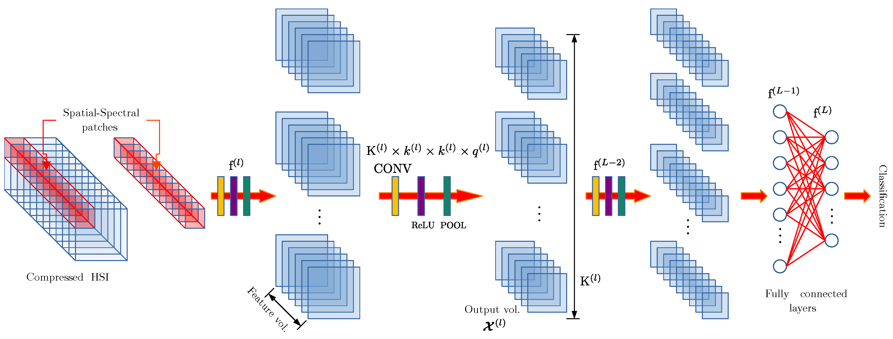
2.3. Spectral–Spatial Deep Learning Models

Generally, spectral signatures of equally labeled pixels are highly correlated between them, and this is a feature that most of the classification algorithms take advantage of for class separation. Spatial correlation is present when a group of neighbor pixels belongs to the same class, which is a common case for remote sensing optical images of the earth surface. Convolutional Neural Networks (CNN) are DL models designed to extract features of neighbor pixels and bands, based on this, the architecture depends on the feature analysis they perform. CNNs for HSI classification are divided in three kinds: spectral, spatial, and spectral–spatial [2].

For the Spectral DL model (1DCNN) in Figure 3, the spectral pixels ${\mathbf{x}}_i\in {\mathbb{N}}^{n_{bands}}$ are the input data, where $n_{bands}$ is the number of bands of the image with or without compression. On each convolutional layer (CONV), 1D-kernels are applied, such that $K^{\left(l\right)}\times q^{\left(l\right)}$, obtaining as a result an output ${\mathbf{X}}^{\left(l\right)}$ composed of $K^{\left(l\right)}$ feature vectors [2].

Spatial DL models (2DCNN) consider the spatial information obtained from the neighbor pixels of the HSI, see Figure 4. For that reason, the input will be spatial patches of $d\times d$ pixels cropped from the complete HSI with the pixel of interest at the center. To extract spatial features, on each CONV layer, 2D-kernels are applied over the input data, such that $K^{\left(l\right)}\times k^{\left(l\right)}\times q^{\left(l\right)}$, obtaining $K^{\left(l\right)}$ feature maps as a result [2].

Spectral–spatial DL models (3DCNN) extract spectral and spatial features at the same time, see Figure 5. Similarly, as with 2DCNN, the features are extracted from spatial patches of $d\times d$, associated with a single pixel of the HSI. This model uses 3D-kernels, such that $K^{\left(l\right)}\times k^{\left(l\right)}\times k^{\left(l\right)}\times q^{\left(l\right)}$, extracting $K^{\left(l\right)}$ feature volumes as output [2].

All these spectral feature extraction DL methods basically infer the ground truths based on the spectral signature. Moreover, remote sensing images exhibit an obvious correlation between neighbor pixels, causing the spatial feature extraction to be a good candidate for this task. Spectral–Spatial feature extraction adopts both characteristics, creating features volumes from a pixel of interest, and, additionally, contains information from its neighbor pixels. For this reason, we use 3DCNN, which is used for the classification of hyperspectral remote sensing noisy images.

2.4. Unbalanced Classification Performance Metrics

Unbalanced classification performance metrics are a key piece for this framework, because we cannot guarantee the same number of labeled samples per each class for HSIs to be tested. Each image will have different spatial Ground Truth (GT) distribution, and there is a need to highlight that, when identifying targets with a low sample count, classical metrics in multi-class classification may show biases. For example, the Overall Accuracy is defined as the number of correct classified samples divided by the overall number of samples. This metric is not reliable when the classification problem is imbalanced. The Average Accuracy metric is essentially an average of the accuracies per each class. If the classification problem shows an unbalanced distribution of classes, this metric takes into account the accuracy per each class as equal, independent of the number of samples. On the other hand, Cohen in 1960 evaluated the classification of two raters (prediction of the model and the actual GT) in order to measure the agreement between them [41]. Cohen’s Kappa coefficient (K) is widely used for the performance evaluation of remote sensing image classification. For this reason, all the results in this work are presented with this metric.

Given a predicted classification map $\widehat{\mathbf{Y}}$, obtained from the trained classifier, and the ground truth $\mathbf{Y}$, of the HSI, a multi-class confusion matrix $\mathbf{M}=\left(m_{i,j}\right)\in {\mathbb{Z}}^{c\times c}$ is computed, where c is the number of classes in $\mathbf{Y}$.

For the case of a binary confusion matrix, Cohen´s Kappa coefficient is defined as follows:

$$K=\frac{P_o-P_e}{1-P_e}.$$

(17)

where $P_o$ is the accuracy achieved by the model, $P_e$ is the level of accuracy to obtain by chance. For a multi-class confusion matrix, K is defined as:

$$K=\frac{{\sum }_{k=1}^c{m}_{k,k}{\sum }_{i=1}^c{\sum }_{j=1}^c{m}_{i,j}-{\sum }_{k=1}^c\left({\sum }_{i=1}^c{m}_{i,k}{\sum }_{j=1}^c{m}_{k,j}\right)}{{\left({\sum }_{i=1}^c{\sum }_{j=1}^c{m}_{i,j}\right)}^2-{\sum }_{k=1}^c\left({\sum }_{i=1}^c{m}_{i,k}{\sum }_{j=1}^c{m}_{k,j}\right)}.$$

(18)

The case when $K=1$ shows a perfect agreement between the GT and predicted labels. $K=0$ means that there is a chance of agreement, but if K is negative, it is a clear disagreement. Each class classification must have importance; for that reason, all the results are presented with Cohen’s Kappa coefficient, but the other two metrics (OA and AA) can be consulted in the log files available in the public repository of this paper [54].

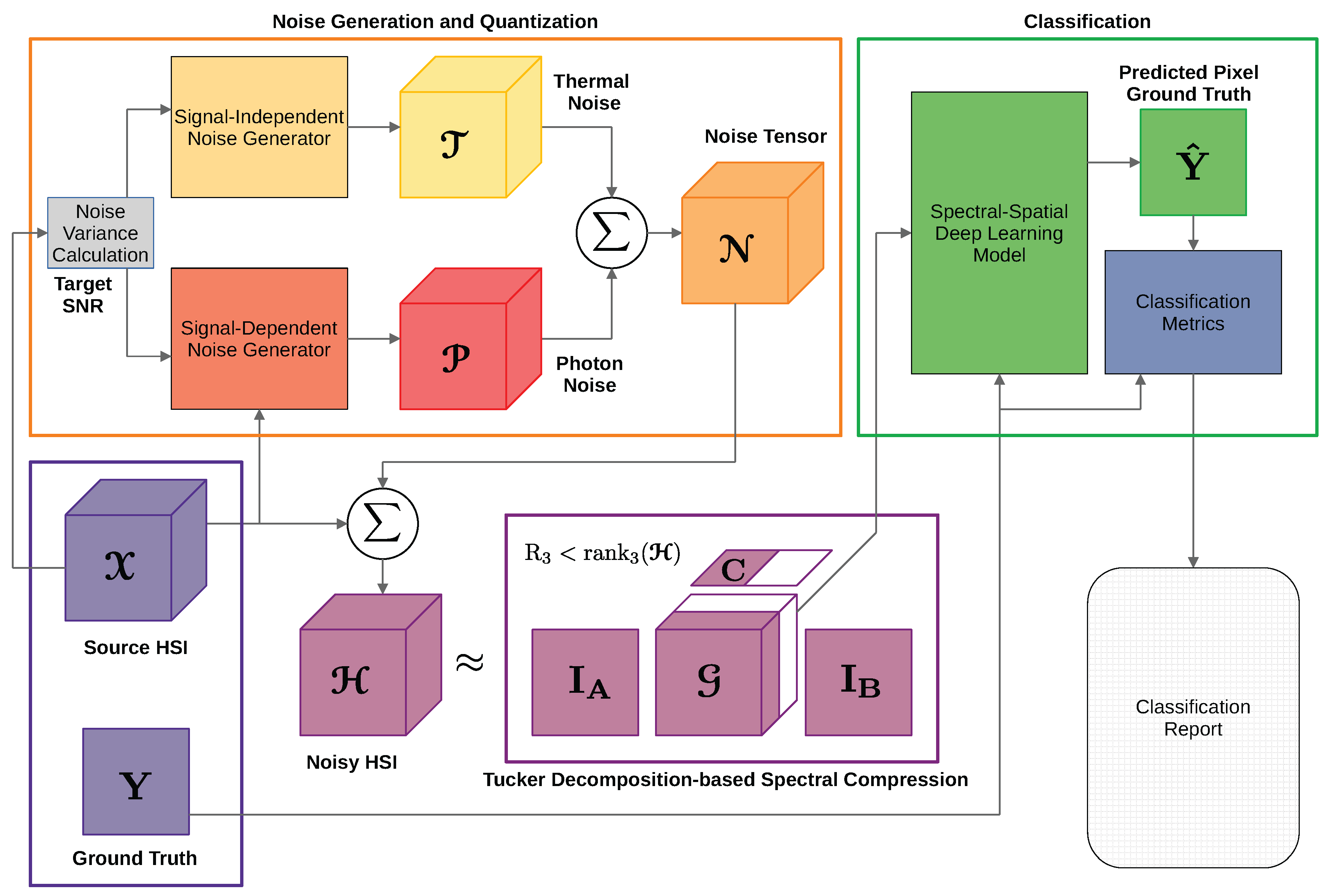
3. Proposed Framework

The proposed framework consists of the following three blocks:

• Noise Generation and Quantization: Having as input the clean signal power, the variances for signal-dependent and independent noise processes are calculated for a specified SNR. In order to follow the non-negative integer values of a digital image, a quantization is performed.
• Tucker Decomposition: Transforms $\mathcal{H}$ into a new input space through a core-tensor $\mathcal{G}$ and factor matrices ${\mathbf{I}}_{\mathbf{A}}$, ${\mathbf{I}}_{\mathbf{B}}$ and $\mathbf{C}$, where $\mathcal{G}$ is a spectrally compressed version of $\mathcal{H}$.
• Deep Learning Model: The model is fitted in terms of the Softmax loss with $\mathcal{G}$ and the class labels present in the ground truth $\mathbf{Y}$, evaluating the prediction $\widehat{\mathbf{Y}}$ of the trained model with metrics that consider a possible unbalanced class scenario.

In Figure 6, a block diagram of the proposed framework is shown.

3.1. Problem Statement

Given $\mathcal{X}\in {\mathbb{R}}^{I_1\times I_2\times I_3}$, which is a source HSI in a third-order tensor form, assuming high-SNR, and $\mathbf{Y}\in {\mathbb{N}}^{I_1\times I_2}$, and given the corresponding pixel ground truth matrix, a noise tensor $\mathcal{N}$ must be generated with the same size of $\mathcal{X}$, $\mathcal{N}\in {\mathbb{R}}^{I_1\times I_2\times I_3}$. $\mathcal{N}$ is the sum of two third-order tensors, the signal-dependent photon noise $\mathcal{P}$, and the signal-independent thermal noise $\mathcal{T}$; hence, $\mathcal{N}=\mathcal{P}+\mathcal{T}$. $\mathcal{N}$ must be generated in such a way that the SNR between $\mathcal{X}$ and $\mathcal{N}$ is at a desired target and the power of both noise tensors are at different proportions. Thus, the new noisy HSI $\mathcal{H}$ is obtained from the sum of the original HSI $\mathcal{X}$, and the generated noise tensor $\mathcal{N}$; therefore, $\mathcal{H}=\mathcal{X}+\mathcal{N},\mathcal{H}\in {\mathbb{R}}^{I_1\times I_2\times I_3}$.

The purpose of $\mathcal{H}$ is to evaluate the classification performance of the Spectral–Spatial DL models when the input HSI is noisy and no denoising method is applied, but the training complexity of these models is too high compared with some classical classifiers. Hence, there is a need to reduce the size of the input to decrease the computational complexity of the DL model. This task could be performed using a Tucker Decomposition-based Spectral Compression, setting a suitable compression ratio. Thus, it is necessary to find a core tensor $\mathcal{G}\in {\mathbb{R}}^{I_1\times I_2\times R_3}$, which will be a spectrally compressed version of $\mathcal{H}$, such that $R_3\le {\mathrm{rank}}_3\left(\mathcal{H}\right)$.

With the pair $(\mathcal{G},\mathbf{Y})$, divide the ground truth available pixels in training and testing sets, taking into account a possible imbalanced classification case. Train the DL Spectral–Spatial Model and predict with it a $\widehat{\mathbf{Y}}$. Finally, evaluate the performance of the DL model with multi-class classification metrics between $\mathbf{Y}$ and $\widehat{\mathbf{Y}}$.

3.2. Noise Generation and Quantization

For experiment purposes of this paper, under the assumption of high-SNR, each available HSI obtained from space agencies is considered as the clean signal $\mathcal{X}$ from Equation (16). From $\mathcal{X}$, the noise variances ${\sigma }_{u,i_3}^2$ and ${\sigma }_{t,i_3}^2$ are calculated to generate samples of the random processes $u_{i_1,i_2,i_3}$ and $t_{i_1,i_2,i_3}$, which correspond to generate the noise tensors ${\mathcal{N}}_{SD}\left(\mathcal{X}\right)$ and ${\mathcal{N}}_{SI}$ at a specified SNR in dB [39]. If the variance of the signal is calculated on homogeneous pixels, this is ${\sigma }_{x_{i_1,i_2,i_3}}^2=0$ by definition [51]; assuming that x, u, and t are independent, and both u and t are zero mean and stationary, the noise variance of each element $n\left(\mathcal{X}\right)$ of the noise tensor $\mathcal{N}\left(\mathcal{X}\right)$ can be written as [39]:

$${\sigma }_{n_{i_1,i_2,i_3}}^2\left(\mathcal{X}\right)=x_{i_1,i_2,i_3}·{\sigma }_{u,i_3}^2+{\sigma }_{t,i_3}^2;$$

(19)

“in practice, homogeneous pixels with ${\sigma }_{x_{i_1,i_2,i_3}}^2=0$ may be extremely rare and theoretical expectation are approximated with local averages” [51]. The mean variance of the noise tensor $\mathcal{N}\left(\mathcal{X}\right)$ is composed of the sum of the SD and SI noise variances:

$${\sigma }_{\mathcal{N}\left(\mathcal{X}\right)}^2={\sigma }_{{\mathcal{N}}_{SD}\left(\mathcal{X}\right)}^2+{\sigma }_{{\mathcal{N}}_{SI}}^2.$$

(20)

Besides, it can be expressed in terms of the mean power of the signal $\mathcal{X}$ and the SNR (dB):

$${\sigma }_{\mathcal{N}\left(\mathcal{X}\right)}^2={\overline{P}}_{\mathcal{X}}·{10}^{-\left(\frac{\mathrm{SNR}}{10}\right)},$$

(21)

where ${\overline{P}}_{\mathcal{X}}=\frac{{\parallel \mathcal{X}\parallel }^2}{I_1{I}_2{I}_3}$. Assuming a parameter $\alpha$, which controls the contribution of both noise processes to the noise tensor $\mathcal{N}\left(\mathcal{X}\right)$, such that:

$$\alpha =\frac{{\sigma }_{{\mathcal{N}}_{SD}\left(\mathcal{X}\right)}^2}{{\sigma }_{{\mathcal{N}}_{SI}}^2}.$$

(22)

From Equations (20) and (22), the mean SI and SD noise variances are expressed in terms of $\alpha$ as follows:

$$\begin{array}{cc}\hfill {\sigma }_{{\mathcal{N}}_{SD}\left(\mathcal{X}\right)}^2& =\frac{{\sigma }_{\mathcal{N}\left(\mathcal{X}\right)}^2·\alpha }{\alpha +1},\hfill \\ \hfill {\sigma }_{{\mathcal{N}}_{SI}}^2& =\frac{{\sigma }_{\mathcal{N}\left(\mathcal{X}\right)}^2}{\alpha +1}.\hfill \end{array}$$

(23)

Furthermore, the noise variances to draw samples are:

$$\begin{array}{c}\hfill {\sigma }_{u,i_3}^2=\frac{{\sigma }_{{\mathcal{N}}_{SD}\left(\mathcal{X}\right)}^2}{{\mu }_{i_3}},\\ \hfill {\sigma }_{t,i_3}^2={\sigma }_{{\mathcal{N}}_{SI}}^2.\end{array}$$

(24)

Some mathematical details of the noise model can be consulted in Appendix A.1.

Once obtained, the noise variances are drawn as random samples from a normal continuous random variable to obtain the tensor $\mathcal{N}$. As seen in Equation (8), $\mathcal{H}$ is obtained by the addition of $\mathcal{X}$ and $\mathcal{N}$. The elements $h_{i_1,i_2,i_3}$ of such tensors are integers, in the range $0\le h_{i_1,i_2,i_3}\le L$, where L is the number of quantization levels, provided by Equation (25), which depends on Q, the number of bits of the sensor. Then,

$$L=2^Q-1,$$

(25)

and where a uniform quantization was performed according to the following rule:

$$h_{i_1,i_2,i_3}=\left\{\begin{array}{cc}0& \mathrm{if}{h}_{i_1,i_2,i_3}\le 0\\ L& \mathrm{if}{h}_{i_1,i_2,i_3}\ge L\\ ⌊h_{i_1,i_2,i_3}⌋& \mathrm{if}\left(h_{i_1,i_2,i_3}-⌊h_{i_1,i_2,i_3}⌋\right)<\frac{1}{2}\\ ⌈h_{i_1,i_2,i_3}⌉& \mathrm{otherwise}.\end{array}\right.$$

(26)

In Figure 7, the behavior of both different kinds of noise is observed, where a specific case of Pavia University is displayed. The SD noise is clearly more present in the high-reflectance pixels. On the other hand, the SI noise is uniformly distributed along the spatial domain.

3.3. Tucker Decomposition-Based Spectral Compression

For our particular case of HSI, we need to reduce the dimensionality in the spectral domain only. If the factor matrices $\mathbf{A}$ and $\mathbf{B}$ are the identity matrices, which correspond to the spatial components, then:

$$\mathcal{H}=\mathcal{G}{\times }_3\mathbf{C}=\left[\left[\mathcal{G};\mathbf{I},\mathbf{I},\mathbf{C}\right]\right],$$

(27)

$${\mathbf{H}}_{\left(3\right)}=\mathbf{C}{\mathbf{G}}_{\left(3\right)}.$$

(28)

Thus, the core tensor keeps the first two dimensions or spatial domain but reduces the third dimension or spectral domain, causing $\mathcal{G}$ to be a spectrally compressed version of $\mathcal{H}$. To perform this computation, using the truncated Tucker Decomposition, set the n-ranks to: $R_1={\mathrm{rank}}_1\left(\mathcal{H}\right)$, $R_2={\mathrm{rank}}_2\left(\mathcal{H}\right)$, and $R_3<{\mathrm{rank}}_3\left(\mathcal{H}\right)$, and reduce the spectral domain from $I_3$ spectral bands to $R_3$ new tensor bands.

3.4. Deep Learning Model Architecture

In this paper, the experiments were performed using a 3DCNN model, given that, generally, the spectral and spatial domains of HSIs are highly correlated. In

Table 2. Architecture of the 3DCNN model.

Main Layer	Normalization	Activation Function	Downsampling
Linear input ($19\times 19\times n_{bands}$)	-	-	-
CONV$\left(32\times 5\times 5\times 24\right)$	BN	ReLU	-
CONV$\left(64\times 5\times 5\times 16\right)$	BN	ReLU	POOL $\left(2\times 2\times 1\right)$
FC$\left(300\right)$	BN	ReLU	-
FC$\left(n_{class}\right)$	-	Softmax	-

, it is shown that the architecture used is [2,10,40]. The fundamentals of the 3DCNN model were explained in Section 2.3.

4. Dataset Experiments and Results

The following section explains the setup and details for the experiments performed to test the framework. The source code and log files with the obtained results are available in the following GitHub repository [54]: github.com/EfrainPadilla, https://github.com/EfrainPadilla/Noisy-Hyperspectral-Semantic-Segmentation-Framework-based-on-Tucker-Decomposition-and-3D-CNN (accessed on 10 March 2022).

4.1. Hardware

The experiments were performed using SSH in a High-Performance Computing (HPC) server installed at the Cinvestav Guadalajara Campus. The hardware is described in

Table 3. Hardware of HPC server for experiments.

Hardware	Cinvestav Guadalajara HPC Server
CPU	×2 Intel Xeon 2.20 GHz 13.75 MB Cache L3
Cores per CPU	10
Threads	40
RAM	6 × 16 GB 96 GB DDR4 HPE Smart 2666 MHz ECC
GPU	×1 NVIDIA Tesla V100 PCIe 3.0
GPU Memory	16 GB HBM2
CUDA cores	5120

. The implementation ran in Python 3.8.5 and the neural network was implemented in Keras-Tensorflow 2.3.0 with CUDA 10.1. Google Collab was used for developing and testing.

4.2. Datasets Description

4.2.1. Indian Pines

The Indian Pines (IP) dataset was captured using the AVIRIS sensor [55] in 1992, an agricultural area in NW Indiana, characterized by its crops of regular geometry and its irregular forest regions. The spatial resolution is 20 m per pixel with dimensions $145\times 145$. From 224 bands in a wavelength range of $0.4$ to $2.5\mathsf{\mu }$m, 24 were removed for being null or water absorption bands (in particular 104–108, 150–163, and 220), considering the remaining 200 bands for the experiments [2]. The ground truth described in

Table 4. Indian Pines ground truth description and true RGB visualization, from [2].

Class Number-Name	Samples	Color	Ground Truth	True RGB
“0-Background	10,776
1-Alfalfa	46
2-Corn-notill	1428
3-Corn-mintill	830
4-Corn	237
5-Grass-pasture	483
6-Grass-trees	730
7-Grass-pasture-mowed	28
8-Hay-windrowed	478
9-Oats	20
10-Soybean-notill	972
11-Soybean-mintill	2455
12-Soybean-clean	593
13-Wheat	205
14-Woods	1265
15-Buildings-Grass-Trees-Drives	386
16-Stone-Steel-Towers”	93

has 10,249 labeled samples divided into 16 classes and true color (RGB) is composed from bands 28, 16, and 9 as red, green, and blue, respectively.

4.2.2. University of Pavia

The campus of the University of Pavia (UP) was captured using the ROSIS sensor [56] in 2002, an urban environment in the North of Italy with multiple solid structures, natural objects, and shadows. The spatial resolution is 1.3 m per pixel with dimensions $610\times 340$ and 103 bands in a wavelength range of from $0.43$ to $8.6\mathsf{\mu }$m. The ground truth described in

Table 5. University of Pavia ground truth description and true RGB visualization, from [2].

Class Number-Name	Samples	Color	Ground Truth	True RGB
“0-Background	164,624
1-Asphalt	6631
2-Meadows	18,649
3-Gravel	2099
4-Trees	3064
5-Painted metal sheets	1345
6-Bare Soil	5029
7-Bitumen	1330
8-Self-Blocking Bricks	3682
9-Shadows”	947

has 42,776 labeled samples divided into nine classes and true color (RGB) is composed from bands 48, 24, and 9 as red, green, and blue, respectively.

4.2.3. Salinas

The Salinas (SAL) HSI was captured using the AVIRIS sensor [55] in 2001 over several agricultural fields in the Salinas Valley, CA, USA. The spatial resolution is 3.7 m per pixel with dimensions $512\times 217$. As in the case of IP, from 224 bands in a wavelength range of from $0.43$ to $8.6\mathsf{\mu }$m, 20 were discarded due to water absorption and noise [2]. The ground truth described in

Table 6. Salinas ground truth description and true RGB visualization, from [2].

Class number-name	Samples	Color	Ground Truth	True RGB
“0-Background	56,975
1-Brocoli-green-weeds-1	2009
2-Brocoli-green-weeds-2	3726
3-Fallow	1976
4-Fallow-rough-plow	1394
5-Fallow-smooth	2678
6-Stubble	3959
7-Celery	3579
8-Grapes-untrained	11,271
9-Soil-vinyard-develop	6203
10-Corn-senesced-green-weeds	3278
11-Lettuce-romaine-4wk	1068
12-Lettuce-romaine-5wk	1927
13-Lettuce-romaine-6wk	916
14-Lettuce-romaine-7wk	1070
15-Vinyard-untrained	7268
16-Vinyard-vertical-trellis”	1807

has 54,129 labeled samples divided into 16 classes and true color (RGB) is composed from bands 28, 16, and 9 as red, green, and blue, respectively.

4.3. Data Pre-Processing for Reduction of Number of Bands

The noise generation is implemented using the random.normal package of Numpy [57], where we draw samples with the computed variances, seen in Section 3.2. Tucker Decomposition is implemented using Tensorly [58], but the code was modified to set the spatial projection matrices to be the identity matrix, as seen in Equation (27). To select the spectral compression ratio, the reconstruction error of the original $\mathcal{H}$ using TKD for different number of tensor bands $R_3=1,2,...,I_3$ was calculated. The relative reconstruction error $\xi$ is obtained using Equation (29).

$$\xi =\frac{\parallel \mathcal{H}-{\widehat{\mathcal{H}}}_{R_3}{\parallel }^2}{{\parallel \mathcal{H}\parallel }^2}.$$

(29)

In Figure 8, the relative reconstruction error is shown for each compression case of IP, UP, and SAL. We have selected $R_3=40$ for all the experiments of this paper, given its low relative reconstruction error (below 1%) for the three images.

Table 7. Reconstruction error and running time of TKD compressing to 40 tensorial bands.

HSI	$\mathit{\xi }$	TKD Running Time (s)
IP	0.994 %	2.89
UP	0.019 %	16.83
SAL	0.027 %	12.41

shows the reconstruction error $\xi$ and the running time of TKD with $R_3=40$, for each HSI used in this paper.

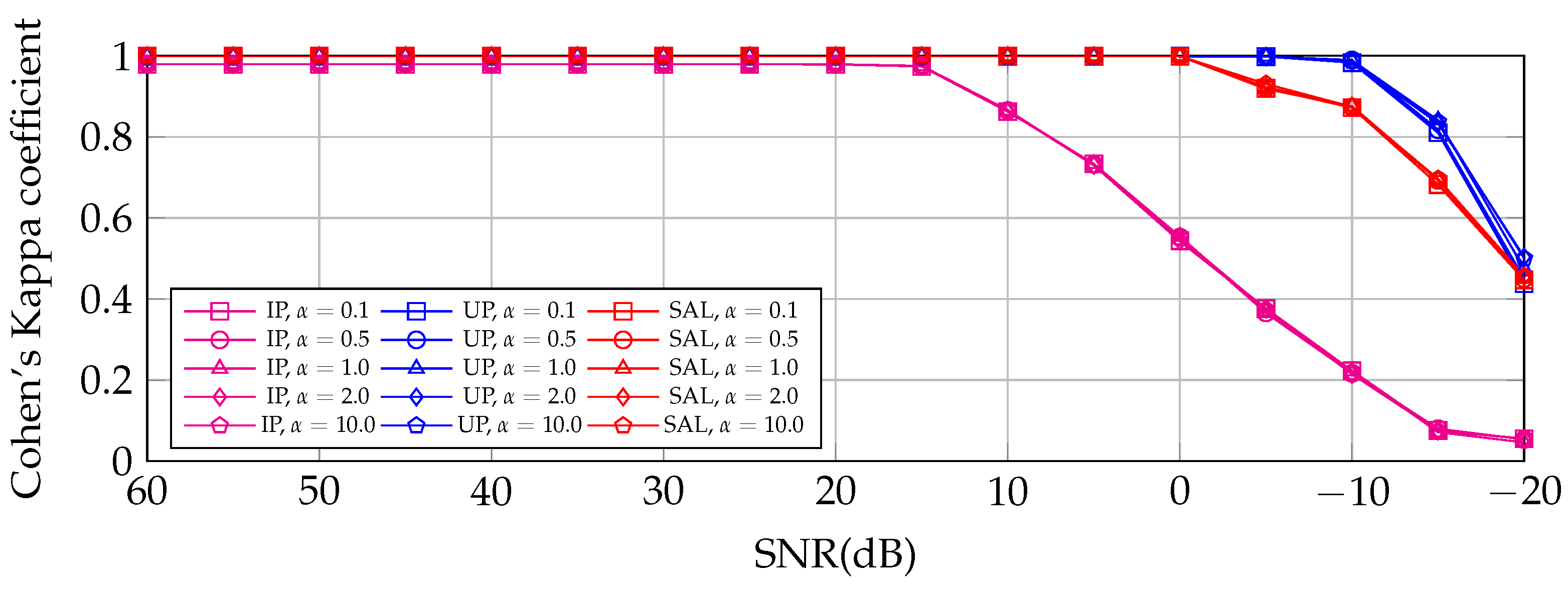
TKD Behavior for Low-SNR HSI Analysis

The aim of the TKD is to find a vector space of a smaller dimension to represent the same information of the original space, taking advantage of the spatial and spectral correlation of pixels. As explained in Section 2, the core tensor $\mathcal{G}$ defines the contribution by the weights on the $i^{th}$ frontal slice ${\mathbf{G}}_{::i}$. A simple way to visualize the contribution of each tensorial band is to compute the power per pixel $p_i$ of the $i^{th}$ frontal slice using $p_i=\frac{\parallel {\mathbf{G}}_{::i}{\parallel }^2}{I_1{I}_2}$. In Figure 9, the behaviors of the contribution for the first tensorial bands from 60 dB to −20 dB are shown for the three datasets used in this paper. The last bands show very low power compared to the first ones; for this reason, they are not included in Figure 9. It is clear that the main contribution is on the first two tensorial bands of $\mathcal{G}$ for the three datasets, but the contribution becomes smaller for low-SNR scenarios. This is explained because the data becomes uncorrelated by the random noise processes with higher variances, causing it to be harder to find a projection matrix that defines the direction of the data. For IP in Figure 9a, the power per pixel of the first tensorial bands start to decay approximately at 20 dB, for UP in Figure 9b at 0 dB, and SAL in Figure 9c at 10 dB; note that SAL decays less than IP and UP. The higher power per pixel values corresponds to high spatial correlated scenes, such as IP and SAL, which are composed of agricultural crops, different to UP, which is an urban scenario. This could explain the power value differences.

To take advantage of the spatial correlation feature extraction of the 3DCNN model, it is necessary to generate a patch with the pixel of interest and its neighbors to train and test the DL model. Each patch $\mathcal{P}$ is composed of 361 pixels ($\mathcal{P}\in {\mathbb{R}}^{19\times 19\times bands}$), with the pixel of interest in the center ($p_{9,9,i_3}$); if this pixel is associated with a background label, the patch is discarded. The patch is padded with zeros if the pixel is at the edge of the image. Note that the labeled patches contain unlabeled pixels. In

Table 8. Running time for patch generation.

Compressed HSI (40 Bands)	Patches Generation Running Time (s)
IP	0.71
UP	18.51
SAL	10.53

, the running time for patch generation is shown.

We have used scikit-learn [59] for the split of patches in the training and testing sets. The samples are randomly chosen in each experiment with a stratification strategy based on k-folds, which returns the stratified folds, where we ensure that the train and test sets have approximately the same percentage of samples of each class available in the ground truth $\mathbf{Y}$. In this paper, the size for the training dataset is called the Train Size (TS), and is represented in a percentage from the total labeled samples available. The size for the testing data will be the remaining labels. In

Table 9. Number of samples for training and testing sets.

HSI	Set	20%	15%	10%	5%	3%	1%
IP	Training	2049	1537	1024	512	-	-
	Testing	8200	8712	9225	9737	-	-
UP	Training	-	6416	4277	2138	1283	427
	Testing	-	36,360	38,499	40,638	41,493	42,349
SAL	Training	-	8118	5412	2706	1623	541
	Testing	-	46,011	48,717	51,423	52,506	53,588

, the number of samples for each case are shown. For the IP case, a smaller set than 5% for the training implies selecting less than one sample for the “Oats” class; for this reason, we do not perform experiments with smaller TS for IP. On the other hand, a bigger TS than 20% for IP or 15% for UP and SAL obtain redundant results and are not aggregated for easy-reading reasons.

4.4. 3DCNN Prediction of Data with Variable SNR from 60 to −20 dB

To test the 3DCNN DL model robustness against noise, this experiment considers the model trained with the original data “clean signal”, but the prediction is performed for noisy data with different SNR levels and $\alpha$ values. The model was trained for IP, UP, and SAL with a TS of 15%; the results are shown in Figure 10.

This experiment shows that the prediction made by 3DCNN does not change significantly when the signal power is greater than the noise power. For IP, noise affects the prediction for SNR ≤ 15 dB. For UP and SAL, noise affects the classifier when the SNR is below 0 dB. The different tested $\alpha$ values do not seem to affect the prediction performance in any particular way.

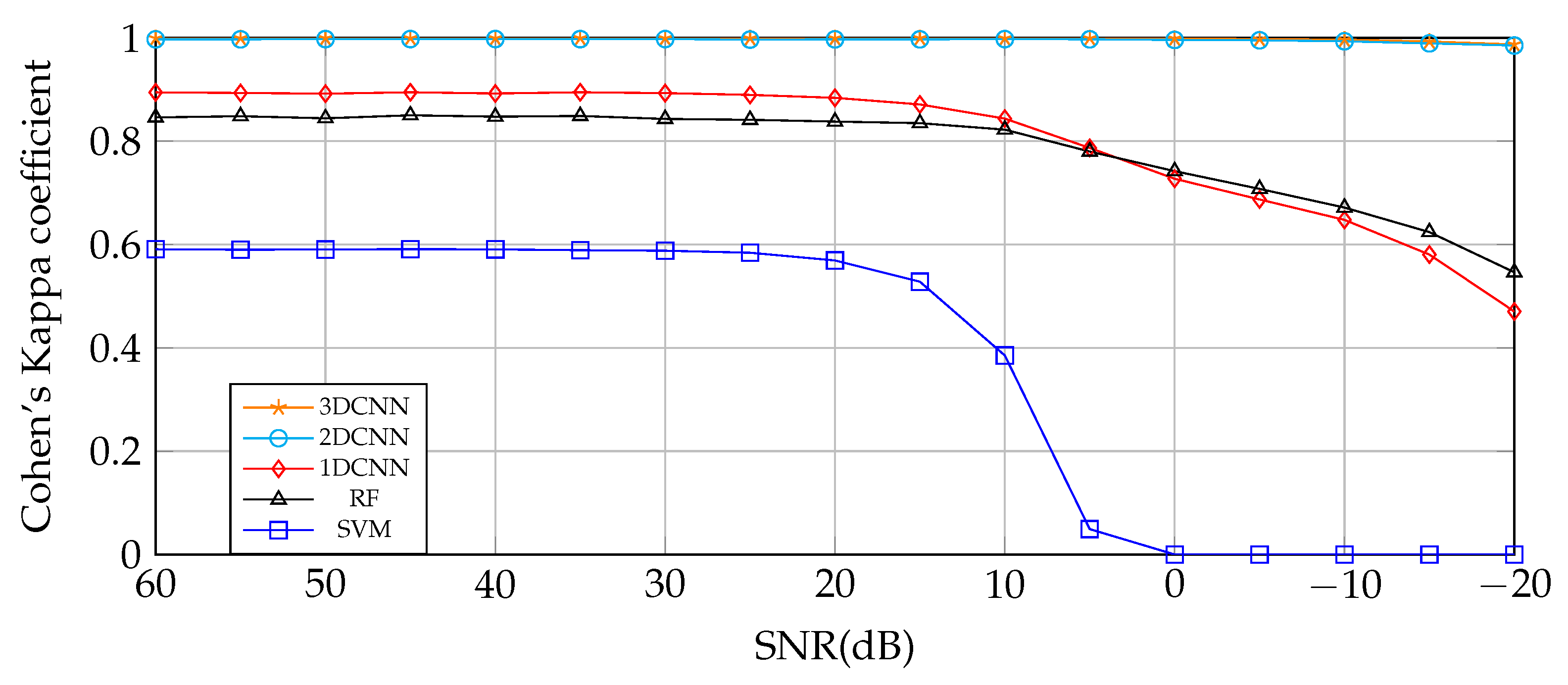
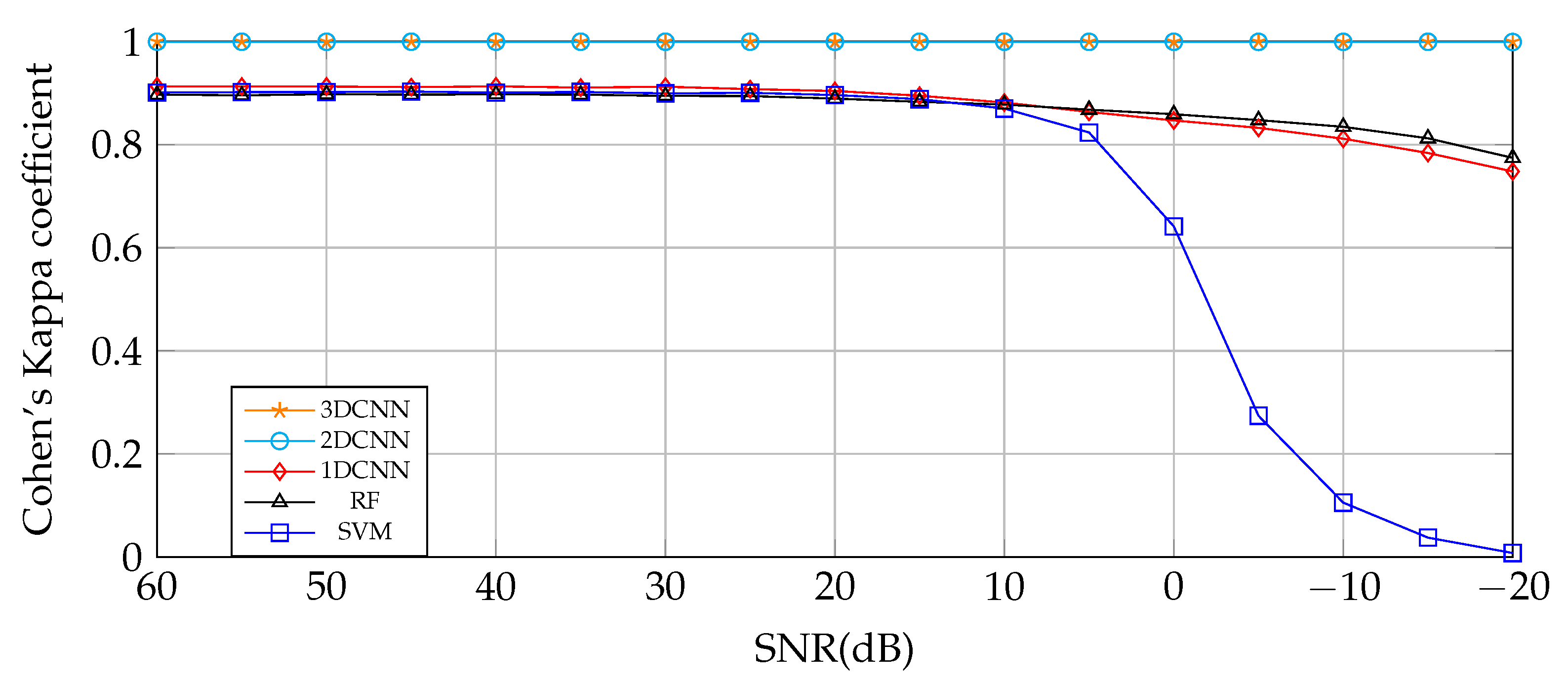
4.5. Comparison between 3DCNN and Other Classical Algorithms

In this section, Figure 11, Figure 12 and Figure 13 show a comparison of the performance robustness to high-level noisy data scenarios of spectral (1DCNN), spatial (2DCNN), and spatial–spectral (3DCNN) DL models; additionally, Random Forest (RF) and Support Vector Machine (SVM), which are widely used classifiers, are tested in the same scenario. The training and testing were individually performed for each SNR level with $\alpha =1$. The results are the average of 10 runs, showing very low variability.

Table A1. Average Cohen’s Kappa coefficient of 10 runs obtained using different classifiers for IP, UP, and SAL compressed with TKD to 40 tensorial bands training with 10% of TS. Standard deviation shows very low variability for high-SNR cases, growing as the noise variance increases.

	SNR	SVM	RF	1DCNN	2DCNN	3DCNN
Indian Pines	60 dB	0.6244 ± 0.0068	0.6664 ± 0.0111	0.6231 ± 0.0113	0.9654 ± 0.0059	0.9802 ± 0.0029
	55 dB	0.6241 ± 0.0087	0.6682 ± 0.0068	0.6250 ± 0.0099	0.9683 ± 0.0024	0.9803 ± 0.0024
	50 dB	0.6303 ± 0.0066	0.6716 ± 0.0105	0.6186 ± 0.0104	0.9690 ± 0.0078	0.9817 ± 0.0040
	45 dB	0.6289 ± 0.0090	0.6697 ± 0.0068	0.6193 ± 0.0086	0.9641 ± 0.0059	0.9793 ± 0.0056
	40 dB	0.6223 ± 0.0029	0.6780 ± 0.0112	0.6203 ± 0.0139	0.9720 ± 0.0045	0.9799 ± 0.0050
	35 dB	0.6148 ± 0.0103	0.6795 ± 0.0075	0.6133 ± 0.0103	0.9712 ± 0.0045	0.9781 ± 0.0029
	30 dB	0.5985 ± 0.0105	0.6660 ± 0.0111	0.6008 ± 0.0061	0.9692 ± 0.0052	0.9793 ± 0.0035
	25 dB	0.5501 ± 0.0100	0.6553 ± 0.0107	0.5803 ± 0.0093	0.9665 ± 0.0043	0.9773 ± 0.0033
	20 dB	0.4354 ± 0.0066	0.6346 ± 0.0092	0.5303 ± 0.0126	0.9660 ± 0.0049	0.9737 ± 0.0059
	15 dB	0.1919 ± 0.0093	0.6054 ± 0.0094	0.4856 ± 0.0108	0.9574 ± 0.0060	0.9673 ± 0.0043
	10 dB	0.0248 ± 0.0037	0.5808 ± 0.0063	0.4419 ± 0.0131	0.9573 ± 0.0068	0.9628 ± 0.0035
	5 dB	0.0006 ± 0.0003	0.5424 ± 0.0069	0.4106 ± 0.0063	0.9493 ± 0.0060	0.9522 ± 0.0061
	0 dB	0.0000 ± 0.0001	0.5086 ± 0.0069	0.3831 ± 0.0128	0.9406 ± 0.0065	0.9425 ± 0.0081
	−5 dB	0.0000 ± 0.0000	0.4664 ± 0.0083	0.3433 ± 0.0120	0.9443 ± 0.0092	0.9404 ± 0.0068
	−10 dB	0.0000 ± 0.0000	0.4191 ± 0.0039	0.2826 ± 0.0130	0.9318 ± 0.0096	0.9299 ± 0.0042
	−15 dB	0.0000 ± 0.0000	0.3700 ± 0.0081	0.2246 ± 0.0085	0.9143 ± 0.0099	0.9083 ± 0.0079
	−20 dB	0.0000 ± 0.0000	0.2938 ± 0.0069	0.1534 ± 0.0099	0.9091 ± 0.0164	0.9002 ± 0.0079
University of Pavia	60 dB	0.5909 ± 0.0048	0.8461 ± 0.0036	0.8946 ± 0.0045	0.9973 ± 0.0009	0.9994 ± 0.0003
	55 dB	0.5900 ± 0.0043	0.8484 ± 0.0037	0.8935 ± 0.0044	0.9972 ± 0.0004	0.9994 ± 0.0003
	50 dB	0.5904 ± 0.0041	0.8444 ± 0.0076	0.8920 ± 0.0061	0.9977 ± 0.0009	0.9995 ± 0.0005
	45 dB	0.5911 ± 0.0033	0.8502 ± 0.0050	0.8948 ± 0.0052	0.9977 ± 0.0004	0.9995 ± 0.0004
	40 dB	0.5906 ± 0.0040	0.8475 ± 0.0089	0.8924 ± 0.0042	0.9978 ± 0.0006	0.9994 ± 0.0003
	35 dB	0.5890 ± 0.0050	0.8489 ± 0.0041	0.8947 ± 0.0069	0.9976 ± 0.0008	0.9996 ± 0.0002
	30 dB	0.5880 ± 0.0034	0.8431 ± 0.0061	0.8931 ± 0.0050	0.9977 ± 0.0005	0.9994 ± 0.0002
	25 dB	0.5841 ± 0.0028	0.8415 ± 0.0040	0.8897 ± 0.0048	0.9967 ± 0.0011	0.9992 ± 0.0004
	20 dB	0.5692 ± 0.0041	0.8380 ± 0.0051	0.8840 ± 0.0083	0.9972 ± 0.0013	0.9995 ± 0.0003
	15 dB	0.5281 ± 0.0016	0.8350 ± 0.0037	0.8713 ± 0.0035	0.9972 ± 0.0008	0.9996 ± 0.0002
	10 dB	0.3853 ± 0.0049	0.8224 ± 0.0032	0.8438 ± 0.0049	0.9977 ± 0.0008	0.9993 ± 0.0003
	5 dB	0.0492 ± 0.0021	0.7800 ± 0.0036	0.7870 ± 0.0045	0.9973 ± 0.0004	0.9993 ± 0.0003
	0 dB	0.0000 ± 0.0000	0.7421 ± 0.0035	0.7274 ± 0.0056	0.9961 ± 0.0011	0.9989 ± 0.0005
	−5 dB	0.0000 ± 0.0000	0.7077 ± 0.0028	0.6873 ± 0.0030	0.9954 ± 0.0011	0.9977 ± 0.0012
	−10 dB	0.0000 ± 0.0000	0.6716 ± 0.0032	0.6478 ± 0.0039	0.9934 ± 0.0018	0.9966 ± 0.0009
	−15 dB	0.0000 ± 0.0000	0.6241 ± 0.0030	0.5806 ± 0.0069	0.9894 ± 0.0013	0.9930 ± 0.0012
	−20 dB	0.0000 ± 0.0000	0.5463 ± 0.0026	0.4703 ± 0.0084	0.9853 ± 0.0028	0.9874 ± 0.0017
Salinas	60 dB	0.9010 ± 0.0021	0.8971 ± 0.0023	0.9131 ± 0.0036	0.9996 ± 0.0004	0.9999 ± 0.0001
	55 dB	0.9017 ± 0.0018	0.8954 ± 0.0026	0.9125 ± 0.0030	0.9995 ± 0.0002	0.9999 ± 0.0001
	50 dB	0.9016 ± 0.0025	0.8977 ± 0.0040	0.9126 ± 0.0025	0.9994 ± 0.0004	0.9999 ± 0.0001
	45 dB	0.9029 ± 0.0021	0.8967 ± 0.0019	0.9114 ± 0.0031	0.9995 ± 0.0002	0.9999 ± 0.0001
	40 dB	0.9006 ± 0.0019	0.8975 ± 0.0020	0.9129 ± 0.0025	0.9995 ± 0.0002	0.9998 ± 0.0001
	35 dB	0.9020 ± 0.0017	0.8968 ± 0.0021	0.9106 ± 0.0041	0.9995 ± 0.0003	0.9999 ± 0.0001
	30 dB	0.8993 ± 0.0019	0.8944 ± 0.0019	0.9122 ± 0.0023	0.9995 ± 0.0003	0.9999 ± 0.0001
	25 dB	0.9003 ± 0.0019	0.8940 ± 0.0028	0.9076 ± 0.0038	0.9995 ± 0.0001	0.9999 ± 0.0001
	20 dB	0.8961 ± 0.0016	0.8892 ± 0.0017	0.9039 ± 0.0026	0.9995 ± 0.0003	0.9999 ± 0.0001
	15 dB	0.8881 ± 0.0012	0.8828 ± 0.0026	0.8947 ± 0.0029	0.9994 ± 0.0003	0.9998 ± 0.0001
	10 dB	0.8699 ± 0.0015	0.8777 ± 0.0015	0.8815 ± 0.0034	0.9996 ± 0.0002	0.9998 ± 0.0001
	5 dB	0.8234 ± 0.0025	0.8677 ± 0.0022	0.8634 ± 0.0041	0.9993 ± 0.0003	0.9998 ± 0.0001
	0 dB	0.6413 ± 0.0035	0.8589 ± 0.0020	0.8468 ± 0.0025	0.9994 ± 0.0003	0.9997 ± 0.0001
	−5 dB	0.2741 ± 0.0100	0.8474 ± 0.0025	0.8324 ± 0.0031	0.9992 ± 0.0003	0.9998 ± 0.0001
	−10 dB	0.1056 ± 0.0013	0.8344 ± 0.0020	0.8114 ± 0.0029	0.9993 ± 0.0003	0.9995 ± 0.0003
	−15 dB	0.0377 ± 0.0005	0.8121 ± 0.0015	0.7837 ± 0.0039	0.9994 ± 0.0003	0.9997 ± 0.0001
	−20 dB	0.0079 ± 0.0005	0.7743 ± 0.0027	0.7478 ± 0.0046	0.9989 ± 0.0004	0.9996 ± 0.0002

in Appendix A.2 shows the average Kappa Coefficient with the standard deviation for each experiment.

Given the high spatial correlation of the agricultural crops present in IP, the classifiers based on spatial feature extraction achieved better results in all the noise level scenarios. Besides, 3DCNN performs slightly better than 2DCNN at low-level noisy data scenarios; on the other hand, at highly noisy scenarios, 2DCNN performs better. The performance of the spectral-based feature extraction classifiers, 1DCNN, RF, and SVM, is considerably lower than 2DCNN and 3DCNN in all cases, and they are severely affected for SNR ≤ 0 dB.

4.6. Performance, Computational Complexity, and Training Time Comparison between Original and Compressed Data Using TKD for 3DCNN Model

The purpose of this section is to show how TKD improves the performance and reduces computational complexity. We have tested the 3DCNN DL model for different noise levels with an equivalent presence of SD and SI noise ($\alpha =1$). The compression is performed reducing from 200 (IP), 103 (UP), and 204 (SAL) bands, to 40 new tensor bands in the three cases and for a relative reconstruction error less than 1%. The DL model is trained for 40 epochs.

For the Indian Pines HSI with 10249 labeled samples available, we show three training scenarios with 15%, 10%, and 5% for the TS of them in Figure 14.

It can be seen that the achieved performance of the DL model training with 15% and 10% of the available labels is always high, even in the high-level noisy scenarios. The Tucker Decomposition improves the classification performance in low- and mid-level noisy scenarios in all the cases. For from 5% to 15% of TS, and from SNR 60 to 0 dB, TKD improves the prediction and is more significant for a TS of 5% than 10% or 15%. The performance achieved, fpr the training with 5% of the labels, is significantly lower than the other two cases, but the TKD remarkably improves the classification performance for low- and mid-level noisy scenarios, while reducing the training time.

For the University of Pavia, HSI with 42,773 labeled samples were available; we show two training scenarios with 5% of TS and 1% in Figure 15.

In this case, a consistent improvement of the training is observed with the data compressed by TKD. The improvement increases as the number of available samples for training decreases.

For the Salinas HSI with 54,129 labeled samples available, we show two training scenarios with 5% and 1% of TS in Figure 16.

The same behavior is observed in the SAL case, where TKD remarkably improves the performance in all noisy scenarios. Furthermore, the improvement is more notorious with a lower quantity of samples for training.

From Figure 14, Figure 15 and Figure 16, for 5% of TS until 0 dB of SNR, the lowest score is achieved by IP and the highest by SAL, while UP is in between these two. In these three cases, TKD improves the classification performance in terms of the Cohen’s Kappa coefficient. The classification performance of the DL model trained with the compressed HSI by TKD achieves slightly better results at high-SNR levels compared with the original HSI, while, at low-SNR values (close to 0 dB), the performance decreases as the noise power increases. It is important to note that the classification results for the input data compressed by TKD follows the trends in Figure 9, where, for low-SNR, the weight of the contribution of the first tensorial bands of SAL is greater than that corresponding to IP and UP. For IP, the improvement of TKD decreased from SNR ≤−5 dB; for UP, when SNR ≤−10 dB, and for SAL, it is always superior. Generally, the aim of compression methods is to reduce the input data size for decreased computational complexity of post-processing algorithms. In this case, TKD not only reduces that complexity but it also improves the classification performance in some cases. The training times of the above experiments are shown in

Table 10. Training time comparison for IP, UP, and SAL datasets.

		15% TS	10% TS	5% TS	1% TS
Indian Pines	Original-200 bands (s)	1889.73	1702.36	1469.47	1284.38
	TKD-40 bands (s)	67.56	63.54	58.43	55.32
	Time reduction ratio	27.97	26.79	25.49	22.56
University of Pavia	Original-103 bands (s)	2987.26	2660.66	2321.35	2041.95
	TKD-40 bands (s)	255.90	239.80	228.65	208.53
	Time reduction ratio	11.67	11.09	10.15	9.79
Salinas	Original-204 bands (s)	9762.00	8783.62	7714.61	6692.29
	TKD-40 bands (s)	328.07	302.23	279.74	266.59
	Time reduction ratio	29.75	29.06	25.57	25.10

. Some of them are not displayed in the graphics because of easy-reading reasons (all the log files are available at the public repository for this paper [54]), but all cases follow the same behavior. TKD reduces the original number of bands of each HSI to 40 tensor bands in all the experiments, with a low relative reconstruction error ($\xi \le 1$%). The times shown in Table 10 are approximately the average of the experiments presented above, the variation of the training time is insignificant in all the experiments with the same TS.

4.7. Framework Testing with Datasets for Different $\alpha$-Values and TS Percentage

The aim of the experiments of this subsection is to show the 3DCNN model performance for different levels and kinds of noise, simulating an extensive set of scenarios for the framework testing. The parameter $\alpha$ controls the dominance of signal-dependent over signal-independent noise (see Equation (22)). The following experiments in Figure 17, Figure 18 and Figure 19 were performed compressing the HSIs to 40 tensor bands and training the 3DCNN DL model for 40 epochs.

These experiments show the capabilities of the DL model to extract representative features for all datasets employed in this work. These results have shown that a representative number of samples of each class for training is key for the consistent performance for SNR ≥ 0 dB. In terms of TS, for IP TS $\ge 10\%$, UP TS $\ge 3\%$, and SAL TS$\ge 3\%$. The changes in the $\alpha$ values tested, from 0.1 to 10, do not seem to influence the classification performance.

5. Discussion

In this paper, we provide a classification framework for remote sensing hyperspectral imagery, which allows for adding simulated signal-dependent and signal-independent noise to test their robustness for different SNR values. This kind of framework allows for performing semantic segmentation for noisy hyperspectral images with different SNR values.

The framework is based on a 3DCNN, which is a spectral–spatial deep learning feature extraction model. This method proved to be robust against the training for low-signal-to-noise ratio cases (even when the noise power is greater than the signal power), see Figure 11, Figure 12 and Figure 13. It is also possible when predicting noisy data from training with noise-free data, such that prediction is affected until the noise power is of the same magnitude as the signal power (SNR close to 0 dB), see Figure 10. However, the computational complexity and resource requirements are higher, compared to other classification algorithms. For that reason, we have implemented spectral compression based on Tucker tensor decomposition, resulting in shorter training times and less hardware resources for implementation.

Tucker Decomposition performs compression correctly until the noise power is of the same magnitude as the signal power, which is a borderline noise case. In most cases, compression, based on TKD, improves the performance of the classifier, see Figure 14, Figure 15 and Figure 16. This improvement is most noticeable when the model is trained with a set of samples in the order from 5% to 3%.

Since remote sensing images present in nature an unbalanced classification problem, all the results were analyzed primarily using the multi-class unbalanced classification metric, the Cohen’s Kappa coefficient, which provides us with a summary of the confusion matrix between the predicted labels and the ground truth of the original image. Three unbalanced hyperspectral images widely studied in the state of the art (described in Table 4, Table 5 and Table 6) were used to generate the noise and to test the framework: University of Pavia, Salinas, and Indian Pines.

In this way, the presented framework can effectively classify images directly from raw data, with high- and low-signal-to-noise ratios. In the state-of-the-art context, this article includes a detailed analysis for different noisy cases and training with low availability of labeled samples. Our current experiments have demonstrated outstanding results. Although, some related papers use the same datasets, a direct comparison is not fair because a different noise model or SNR are used, with a different number of samples for the classifier training as well as different objectives. The work closest to us is [25], but it is only comparable with the original datasets or high-SNR cases of Figure 14, Figure 15 and Figure 16, where our approach obtains slightly higher results in terms of the Kappa coefficient for UP (from 0.954 to 0.958) and SAL (from 0.965 to 0.988), but slightly lower results for IP, (from 0.94 to 0.91). For the same original datasets, our approach is competitive with other approaches such as [26,27,28,29,30]. As some of the references present their classification results with the overall accuracy metric only, we prefer to present the results in terms of the Kappa coefficient, because this metric does not hide the imbalanced classification problem.

6. Conclusions

All the results and behaviors can be summarized in the following four conclusions:

• This framework, based on a 3DCNN spectral–spatial deep learning feature extraction model and Tucker Decomposition, proved to be robust in most cases for different combinations and levels of simulated signal-dependent and signal-independent noises, even when the SNR is close to 0 dB.
• Tucker Decomposition reduces from 103 to 224 bands to 40 new tensor bands with $\xi <1$%, reducing the computational complexity for the classifier. Different to other compression algorithms, Tucker Decomposition does not affect the performance of the deep learning model; conversely, it improves the classification performance of the 3DCNN deep learning model in the three studied datasets. This improvement is more noticeable for the training set size in the order of from 5% to 3% for the three datasets tested.
• Tucker Decomposition performs well until SNR is close to 0 dB; for $\mathrm{SNR}\le$ 0 dB, TKD cannot represent the useful information in the core tensor, resulting in an obvious loss of performance.
• With a representative number of labeled samples of each class (depending on the hyperspectral image and accuracy we want), for an SNR ≥ of 0 dB, our proposal is not affected by different $\alpha$-values; in other words, different noisy scenarios of signal-dependent and signal-independent noise.

Open Issues

• To test the spatial–spectral feature extraction of 3DCNN in other types of applications for hyperspectral imagery.
• An algorithm is needed to find the minimum n-rank that fully represents the data into the core tensor, reducing the computational and spatial complexity for posterior stages in the framework.
• To test the framework with a larger number of hyperspectral images, considering distributions of ground truth with less spatial correlation, and for RGB and multi-spectral imagery.
• Mathematical and statistical analysis of Tucker Decomposition for noisy data.

References

1. Borengasser, M.; Hungate, W.S.; Watkins, R.L. Hyperspectral Remote Sensing: Principles and Applications; CRC Press: Boca Raton, FL, USA, 2008; p. 119. [Google Scholar]
2. Paoletti, M.E.; Haut, J.M.; Plaza, J.; Plaza, A. Deep learning classifiers for hyperspectral imaging: A review. ISPRS J. Photogramm. Remote Sens. 2019, 158, 279–317. [Google Scholar] [CrossRef]
3. Rasti, B.; Scheunders, P.; Ghamisi, P.; Licciardi, G.; Chanussot, J. Noise Reduction in Hyperspectral Imagery: Overview and Application. Remote Sens. 2018, 10, 482. [Google Scholar] [CrossRef] [Green Version]
4. Bourennane, S.; Fossati, C.; Lin, T. Noise Removal Based on Tensor Modelling for Hyperspectral Image Classification. Remote Sens. 2018, 10, 1330. [Google Scholar] [CrossRef] [Green Version]
5. Gu, S.; Zhang, L.; Zuo, W.; Feng, X. Weighted nuclear norm minimization with application to image denoising. In Proceedings of the IEEE Computer Society Conference on Computer Vision and Pattern Recognition, Columbus, OH, USA, 23–28 June 2014; IEEE Computer Society: Washington, DC, USA, 2014; pp. 2862–2869. [Google Scholar] [CrossRef] [Green Version]
6. Karami, A.; Yazdi, M.; Zolghadre Asli, A. Noise reduction of hyperspectral images using kernel non-negative tucker decomposition. IEEE J. Sel. Top. Signal Process. 2011, 5, 487–493. [Google Scholar] [CrossRef]
7. Yuan, Q.; Zhang, Q.; Li, J.; Shen, H.; Zhang, L. Hyperspectral image denoising employing a spatial-spectral deep residual convolutional neural network. IEEE Trans. Geosci. Remote Sens. 2019, 57, 1205–1218. [Google Scholar] [CrossRef] [Green Version]
8. Fan, H.; Li, C.; Guo, Y.; Kuang, G.; Ma, J. Spatial-Spectral Total Variation Regularized Low-Rank Tensor Decomposition for Hyperspectral Image Denoising. IEEE Trans. Geosci. Remote Sens. 2018, 56, 6196–6213. [Google Scholar] [CrossRef]
9. Huang, Z.; Li, S.; Fang, L.; Li, H.; Benediktsson, J.A. Hyperspectral Image Denoising with Group Sparse and Low-Rank Tensor Decomposition. IEEE Access 2017, 6, 1380–1390. [Google Scholar] [CrossRef]
10. Chen, Y.; Jiang, H.; Li, C.; Jia, X.; Ghamisi, P. Deep Feature Extraction and Classification of Hyperspectral Images Based on Convolutional Neural Networks. IEEE Trans. Geosci. Remote Sens. 2016, 54, 6232–6251. [Google Scholar] [CrossRef] [Green Version]
11. Hu, J.; Li, L.; Lin, Y.; Wu, F.; Zhao, J. A Comparison and Strategy of Semantic Segmentation on Remote Sensing Images. Adv. Intell. Syst. Comput. 2019, 1074, 21–29. [Google Scholar] [CrossRef] [Green Version]
12. Niu, Z.; Liu, W.; Zhao, J.; Jiang, G. DeepLab-Based Spatial Feature Extraction for Hyperspectral Image Classification. IEEE Geosci. Remote Sens. Lett. 2019, 16, 251–255. [Google Scholar] [CrossRef]
13. Zhong, Z.; Li, J.; Ma, L.; Jiang, H.; Zhao, H. Deep residual networks for hyperspectral image classification. In Proceedings of the International Geoscience and Remote Sensing Symposium (IGARSS), Fort Worth, TX, USA, 23–28 July 2017; Institute of Electrical and Electronics Engineers Inc.: Piscataway, NJ, USA, 2017; pp. 1824–1827. [Google Scholar] [CrossRef] [Green Version]
14. Feng, J.; Yu, H.; Wang, L.; Cao, X.; Zhang, X.; Jiao, L. Classification of Hyperspectral Images Based on Multiclass Spatial-Spectral Generative Adversarial Networks. IEEE Trans. Geosci. Remote Sens. 2019, 57, 5329–5343. [Google Scholar] [CrossRef]
15. Hu, W.; Huang, Y.; Wei, L.; Zhang, F.; Li, H. Deep convolutional neural networks for hyperspectral image classification. J. Sens. 2015, 2015, 258619. [Google Scholar] [CrossRef] [Green Version]
16. Xiao, H.; Wei, Y.; Liu, Y.; Zhang, M.; Feng, J. Transferable Semi-Supervised Semantic Segmentation. Proc. AAAI Conf. Artif. Intell. 2018, 32, 7420–7427. [Google Scholar] [CrossRef]
17. Sun, R.; Zhu, X.; Wu, C.; Huang, C.; Shi, J.; Ma, L. Not all areas are equal: Transfer learning for semantic segmentation via hierarchical region selection. In Proceedings of the IEEE Computer Society Conference on Computer Vision and Pattern Recognition, Long Beach, CA, USA, 15–19 June 2019; pp. 4355–4364. [Google Scholar] [CrossRef]
18. Stan, S.; Rostami, M. Unsupervised Model Adaptation for Continual Semantic Segmentation. Proc. AAAI Conf. Artif. Intell. 2021, 35, 2593–2601. [Google Scholar] [CrossRef]
19. Sun, J.; Wei, D.; Ma, K.; Wang, L.; Zheng, Y. Boost Supervised Pretraining for Visual Transfer Learning: Implications of Self-Supervised Contrastive Representation Learning. Proc. AAAI Conf. Artif. Intell. 2022, 36, 2307–2315. [Google Scholar] [CrossRef]
20. Cui, B.; Chen, X.; Lu, Y. Semantic Segmentation of Remote Sensing Images Using Transfer Learning and Deep Convolutional Neural Network with Dense Connection. IEEE Access 2020, 8, 116744–116755. [Google Scholar] [CrossRef]
21. Ronneberger, O.; Fischer, P.; Brox, T. U-Net: Convolutional Networks for Biomedical Image Segmentation. In Medical Image Computing and Computer-Assisted Intervention—MICCAI 2015; Lecture Notes in Computer Science (Including Subseries Lecture Notes in Artificial Intelligence and Lecture Notes in Bioinformatics); Springer: Cham, Switzerland, 2015; Volume 9351, pp. 234–241. [Google Scholar] [CrossRef] [Green Version]
22. Pasquali, G.; Iannelli, G.C.; Dell’Acqua, F. Building Footprint Extraction from Multispectral, Spaceborne Earth Observation Datasets Using a Structurally Optimized U-Net Convolutional Neural Network. Remote Sens. 2019, 11, 2803. [Google Scholar] [CrossRef] [Green Version]
23. Wieland, M.; Li, Y.; Martinis, S. Multi-sensor cloud and cloud shadow segmentation with a convolutional neural network. Remote Sens. Environ. 2019, 230, 111203. [Google Scholar] [CrossRef]
24. Giang, T.L.; Dang, K.B.; Le, Q.T.; Nguyen, V.G.; Tong, S.S.; Pham, V.M. U-net convolutional networks for mining land cover classification based on high-resolution UAV imagery. IEEE Access 2020, 8, 186257–186273. [Google Scholar] [CrossRef]
25. Fu, H.; Zhang, A.; Sun, G.; Ren, J.; Jia, X.; Pan, Z.; Ma, H. A Novel Band Selection and Spatial Noise Reduction Method for Hyperspectral Image Classification. IEEE Trans. Geosci. Remote Sens. 2022, 60, 1–13. [Google Scholar] [CrossRef]
26. Prasad, S.; Li, W.; Fowler, J.E.; Bruce, L.M. Information fusion in the redundant-wavelet-transform domain for noise-robust hyperspectral classification. IEEE Trans. Geosci. Remote Sens. 2012, 50, 3474–3486. [Google Scholar] [CrossRef]
27. Duan, P.; Kang, X.; Li, S.; Ghamisi, P. Noise-robust hyperspectral image classification via multi-scale total variation. IEEE J. Sel. Top. Appl. Earth Obs. Remote Sens. 2019, 12, 1948–1962. [Google Scholar] [CrossRef]
28. Gong, Z.; Zhong, P.; Yao, W.; Zhou, W.; Qi, J.; Hu, P. A CNN with noise inclined module and denoise framework for hyperspectral image classification. IET Image Process. 2022. [Google Scholar] [CrossRef]
29. Chen, C.; Li, W.; Tramel, E.W.; Cui, M.; Prasad, S.; Fowler, J.E. Spectral–Spatial Preprocessing Using Multihypothesis Prediction for Noise-Robust Hyperspectral Image Classification. IEEE J. Sel. Top. Appl. Earth Obs. Remote Sens. 2014, 7, 1047–1059. [Google Scholar] [CrossRef]
30. Gao, L.; Zhao, B.; Jia, X.; Liao, W.; Zhang, B.; Wang, Q.; Younan, N.H.; López-Martínez, C.; Thenkabail, P.S. Optimized Kernel Minimum Noise Fraction Transformation for Hyperspectral Image Classification. Remote Sens. 2017, 9, 548. [Google Scholar] [CrossRef] [Green Version]
31. Fu, P.; Sun, X.; Sun, Q. Hyperspectral Image Segmentation via Frequency-Based Similarity for Mixed Noise Estimation. Remote Sens. 2017, 9, 1237. [Google Scholar] [CrossRef] [Green Version]
32. de Los Reyes, R.; Langheinrich, M.; Schwind, P.; Richter, R.; Pflug, B.; Bachmann, M.; Müller, R.; Carmona, E.; Zekoll, V.; Reinartz, P. PACO: Python-Based Atmospheric COrrection. Sensors 2020, 20, 1428. [Google Scholar] [CrossRef] [Green Version]
33. Zekoll, V.; Main-Knorn, M.; Alonso, K.; Louis, J.; Frantz, D.; Richter, R.; Pflug, B. Comparison of Masking Algorithms for Sentinel-2 Imagery. Remote Sens. 2021, 13, 137. [Google Scholar] [CrossRef]
34. Guanter, L.; Kaufmann, H.; Segl, K.; Foerster, S.; Rogass, C.; Chabrillat, S.; Kuester, T.; Hollstein, A.; Rossner, G.; Chlebek, C.; et al. The EnMAP Spaceborne Imaging Spectroscopy Mission for Earth Observation. Remote Sens. 2015, 7, 8830–8857. [Google Scholar] [CrossRef] [Green Version]
35. Alonso, K.; Bachmann, M.; Burch, K.; Carmona, E.; Cerra, D.; de los Reyes, R.; Dietrich, D.; Heiden, U.; Hölderlin, A.; Ickes, J.; et al. Data Products, Quality and Validation of the DLR Earth Sensing Imaging Spectrometer (DESIS). Sensors 2019, 19, 4471. [Google Scholar] [CrossRef] [Green Version]
36. López, J.; Torres, D.; Santos, S.; Atzberger, C. Spectral Imagery Tensor Decomposition for Semantic Segmentation of Remote Sensing Data through Fully Convolutional Networks. Remote Sens. 2020, 12, 517. [Google Scholar] [CrossRef] [Green Version]
37. Padilla-Zepeda, E.; Torres-Roman, D.; Mendez-Vazquez, A. Noise analysis using Tucker decomposition and PCA on spectral images. ECORFAN J.-Boliv. 2020, 7, 10–16. [Google Scholar] [CrossRef]
38. Kolda, T.G.; Bader, B.W. Tensor decompositions and applications. SIAM Rev. 2009, 51, 455–500. [Google Scholar] [CrossRef]
39. Liu, X.; Bourennane, S.; Fossati, C. Reduction of signal-dependent noise from hyperspectral images for target detection. IEEE Trans. Geosci. Remote Sens. 2014, 52, 5396–5411. [Google Scholar] [CrossRef]
40. Li, Y.; Zhang, H.; Shen, Q. Spectral–Spatial Classification of Hyperspectral Imagery with 3D Convolutional Neural Network. Remote Sens. 2017, 9, 67. [Google Scholar] [CrossRef] [Green Version]
41. Grandini, M.; Bagli, E.; Visani, G. Metrics for Multi-Class Classification: An Overview. arXiv 2020, arXiv:2008.05756. [Google Scholar]
42. Luque, A.; Carrasco, A.; Martín, A.; de las Heras, A. The impact of class imbalance in classification performance metrics based on the binary confusion matrix. Pattern Recognit. 2019, 91, 216–231. [Google Scholar] [CrossRef]
43. Gonzalez-Ramirez, A.; Lopez, J.; Torres-Roman, D.; Yañez-Vargas, I. Analysis of multi-class classification performance metrics for remote sensing imagery imbalanced datasets. ECORFAN J. Quant. Stat. Anal. 2021, 8, 11–17. [Google Scholar] [CrossRef]
44. Makantasis, K.; Doulamis, A.D.; Doulamis, N.D.; Nikitakis, A. Tensor-based classification models for hyperspectral data analysis. IEEE Trans. Geosci. Remote Sens. 2018, 56, 6884–6898. [Google Scholar] [CrossRef]
45. Sidiropoulos, N.D.; De Lathauwer, L.; Fu, X.; Huang, K.; Papalexakis, E.E.; Faloutsos, C. Tensor Decomposition for Signal Processing and Machine Learning. IEEE Trans. Signal Process. 2017, 65, 3551–3582. [Google Scholar] [CrossRef]
46. An, J.; Lei, J.; Song, Y.; Zhang, X.; Guo, J. Tensor Based Multiscale Low Rank Decomposition for Hyperspectral Images Dimensionality Reduction. Remote Sens. 2019, 11, 1485. [Google Scholar] [CrossRef] [Green Version]
47. Kong, X.; Zhao, Y.; Xue, J.; Chan, J.C.W. Hyperspectral Image Denoising Using Global Weighted Tensor Norm Minimum and Nonlocal Low-Rank Approximation. Remote Sens. 2019, 11, 2281. [Google Scholar] [CrossRef] [Green Version]
48. Lu, H.; Plataniotis, K.N.; Venetsanopoulos, A.N. MPCA: Multilinear principal component analysis of tensor objects. IEEE Trans. Neural Netw. 2008, 19, 18–39. [Google Scholar] [CrossRef] [PubMed] [Green Version]
49. AVIRIS—eoPortal Directory—Airborne Sensors. Available online: https://aviris.jpl.nasa.gov/ (accessed on 15 June 2020).
50. Tucker, L.R. Some mathematical notes on three-mode factor analysis. Psychometrika 1966, 31, 279–311. [Google Scholar] [CrossRef] [PubMed]
51. Alparone, L.; Selva, M.; Aiazzi, B.; Baronti, S.; Butera, F.; Chiarantini, L. Signal-dependent noise modelling and estimation of new-generation imaging spectrometers. In Proceedings of the WHISPERS ’09—1st Workshop on Hyperspectral Image and Signal Processing: Evolution in Remote Sensing, Grenoble, France, 26–28 August 2009. [Google Scholar] [CrossRef]
52. Faraji, H.; MacLean, W.J. CCD noise removal in digital images. IEEE Trans. Image Process. 2006, 15, 2676–2685. [Google Scholar] [CrossRef]
53. Jain, A.K. Fundamentals of Digital Image Processing; Prentice-Hall, Inc.: Hoboken, NJ, USA, 1989. [Google Scholar]
54. Padilla-Zepeda, E. Noisy-Hyperspectral-Semantic-Segmentation-Framework-Based-on-Tucker-Decomposition-and-3D-CNN. 2022. Available online: https://github.com/EfrainPadilla/Noisy-Hyperspectral-Semantic-Segmentation-Framework-based-on-Tucker-Decomposition-and-3D-CNN (accessed on 10 March 2022).
55. Green, R.O.; Eastwood, M.L.; Sarture, C.M.; Chrien, T.G.; Aronsson, M.; Chippendale, B.J.; Faust, J.A.; Pavri, B.E.; Chovit, C.J.; Solis, M.; et al. Imaging spectroscopy and the Airborne Visible/Infrared Imaging Spectrometer (AVIRIS). Remote Sens. Environ. 1998, 65, 227–248. [Google Scholar] [CrossRef]
56. Kunkel, B.; Blechinger, F.; Lutz, R.; Doerffer, R.; van der Piepen, H.; Schroder, M. ROSIS (Reflective Optics System Imaging Spectrometer) - A Candidate Instrument For Polar Platform Missions. Optoelectron. Technol. Remote Sens. Space SPIE 1988, 868, 134. [Google Scholar] [CrossRef]
57. Harris, C.R.; Millman, K.J.; van der Walt, S.J.; Gommers, R.; Virtanen, P.; Cournapeau, D.; Wieser, E.; Taylor, J.; Berg, S.; Smith, N.J.; et al. Array programming with NumPy. Nature 2020, 585, 357–362. [Google Scholar] [CrossRef]
58. Kossaifi, J.; Panagakis, Y.; Anandkumar, A.; Pantic, M. TensorLy: Tensor Learning in Python. J. Mach. Learn. Res. 2019, 20, 1–6. [Google Scholar]
59. Pedregosa, F.; Varoquaux, G.; Gramfort, A.; Michel, V.; Thirion, B.; Grisel, O.; Blondel, M.; Prettenhofer, P.; Weiss, R.; Dubourg, V.; et al. Scikit-learn: Machine Learning in Python. J. Mach. Learn. Res. 2011, 12, 2825–2830. [Google Scholar]
Figure 1. AVIRIS HSI of Indian Pines, NW Indiana. NASA/JPL [49].
Remotesensing 15 01399 g001
Figure 2. Tucker Decomposition of Indian Pines HSI, a third-order tensor.
Remotesensing 15 01399 g002
Figure 3. Traditional architecture of spectral convolutional model employed using 1DCNN [2].
Remotesensing 15 01399 g003
Figure 4. Traditional architecture of spatial convolutional model employed using 2DCNN [2].
Remotesensing 15 01399 g004
Figure 5. Traditional architecture of spectral–spatial convolutional model employed using 3DCNN [2].
Remotesensing 15 01399 g005
Figure 6. Proposed framework.
Remotesensing 15 01399 g006
Figure 7. 30th band of Pavia University HSI. S N R = 15 , α = 5 .
Remotesensing 15 01399 g007
Figure 8. Relative error between original data and the reconstruction from core tensor.
Remotesensing 15 01399 g008
Figure 9. First five tensorial bands power from G , after performing TKD from 60 dB to −20 dB, α = 1 .
Remotesensing 15 01399 g009
Figure 10. Cohen’s Kappa coefficient obtained by the prediction of the 3DCNN DL model over raw noisy data, trained with 15% of the noise-free data of IP, UP, and SAL, without TKD. UP shows the highest Cohen’s Kappa coefficient values until −20 dB; after that SAL and IP are the lowest.
Remotesensing 15 01399 g010
Figure 11. Indian Pines. Cohen’s Kappa coefficient obtained by different classifiers for IP HSI compressed with TKD to 40 tensorial bands training with 10% of TS. The best performance is achieved by 3DCNN and 2DCNN, then RF, 1DCNN, and SVM in descending order.
Remotesensing 15 01399 g011
Figure 12. University of Pavia. Cohen’s Kappa coefficient obtained by different classifiers for UP HSI compressed with TKD to 40 tensorial bands training with 10% of TS. The best performance is achieved by 3DCNN and 2DCNN, then 1DCNN, RF, and SVM in descending order.
Remotesensing 15 01399 g012
Figure 13. Salinas. Cohen’s Kappa coefficient obtained by different classifiers for SAL HSI compressed with TKD to 40 tensorial bands training with 10% of TS. The best performance is achieved by 3DCNN and 2DCNN, then 1DCNN, RF, and SVM show aproximately the same performance above 10 dB, but, below that, SVM was shown to be the worst.
Remotesensing 15 01399 g013
Figure 14. Indian Pines. Cohen’s Kappa coefficient obtained using 3DCNN DL model trained for 40 epochs from the original IP HSI and compressed with TKD to 40 tensorial bands. From 60 to −5 dB, Tucker improved the performance for Cohen’s Kappa coefficient.
Remotesensing 15 01399 g014
Figure 15. University of Pavia. Cohen’s Kappa coefficient obtained using 3DCNN DL model trained for 40 epochs from the original UP HSI and compressed with TKD to 40 tensorial bands. From 60 to −5 dB, Tucker improved the performance for Cohen’s Kappa coefficient.
Remotesensing 15 01399 g015
Figure 16. Salinas. Cohen’s Kappa coefficient obtained using the 3DCNN DL model trained for 40 epochs from the original SAL HSI and compressed with TKD to 40 tensorial bands. From 60 to −20 dB, Tucker improved the performance for Cohen’s Kappa coefficient.
Remotesensing 15 01399 g016
Figure 17. Indian Pines. Cohen’s Kappa coefficient obtained using 3DCNN DL model trained with 20%, 15%, 10%, and 5% of the samples of compressed IP HSI for different α values. α -values do not seem to influence Cohen’s Kappa coefficient.
Remotesensing 15 01399 g017
Figure 18. University of Pavia. Cohen’s Kappa coefficient obtained using 3DCNN DL model trained with 15%, 10%, 5%, 3%, and 1% of the samples of compressed UP HSI for different α values. α -values do not seem to influence on Cohen’s Kappa coefficient.
Remotesensing 15 01399 g018
Figure 19. Salinas. Cohen’s Kappa coefficient obtained using 3DCNN DL model trained with 10%, 5%, 3%, and 1% of the samples of compressed SAL HSI for different α values. α -values do not seem to influence Cohen’s Kappa coefficient.
Remotesensing 15 01399 g019