Article

A Multi-Satellite Mapping Framework for Floating Kelp Forests

1
SPECTRAL Remote Sensing Laboratory, University of Victoria, 3800 Finnerty Road, Victoria, BC V8P 5C2, Canada
2
Canadian Hydrographic Service, Institute of Ocean Sciences, 9860 West Saanich Rd, Sidney, BC V8L 4B2, Canada
3
Hakai Institute, Campbell River, BC V0P 1H0, Canada
*
Author to whom correspondence should be addressed.
Remote Sens. 2023, 15(5), 1276; https://doi.org/10.3390/rs15051276
Submission received: 1 December 2022 / Revised: 11 February 2023 / Accepted: 12 February 2023 / Published: 25 February 2023

Abstract

:
Kelp forests provide key habitat on the Pacific Coast of Canada; however, the long-term changes in their distribution and abundance remain poorly understood. With advances in satellite technology, floating kelp forests can now be monitored across large-scale areas. We present a methodological framework using an object-based image analysis approach that enables the combination of imagery from multiple satellites at different spatial resolutions and temporal coverage, to map kelp forests with floating canopy through time. The framework comprises four steps: (1) compilation and quality assessment; (2) preprocessing; (3) an object-oriented classification; and (4) an accuracy assessment. Additionally, the impact of spatial resolution on the detectability of floating kelp forests is described. Overall, this workflow was successful in producing accurate maps of floating kelp forests, with global accuracy scores of between 88% and 94%. When comparing the impact of resolution on detectability, lower resolutions were less reliable at detecting small kelp forests in high slope areas. Based on the analysis, we suggest removing high slope areas (11.4%) from time series analyses using high- to medium-resolution satellite imagery and that error, in this case up to 7%, be considered when comparing imagery at different resolutions in low–mid slope areas through time.

1. Introduction

Kelp, brown algae in the order Laminariales, are dominant habitat-forming organisms found in cool waters across approximately one-third of the Earth’s coastlines [1,2,3]. Kelp create extensive aquatic forests that provide shelter and food for ecologically and economically important species [1,4,5]. Additionally, kelp provide myriad ecosystem goods and services, such as fisheries production, nutrient cycling and carbon removal, estimated at USD 684 billion per year worldwide [6,7]. However, climate change, overfishing, pollution and increasing harvest threaten the health and persistence of kelp forests globally [1,5,8]. Recent work highlights the negative impacts of heatwaves on kelp forests [9,10,11,12,13,14] and the loss of key predators, such as sea otters and sea stars, leading to overgrazing-induced regime shifts from kelp forests to urchin barrens [6,15,16,17].
Kelp forests are dynamic by nature and show high interannual variability [18,19,20]. Considering that kelp forests are threatened globally, but are highly variable through time, it is important to establish long-term time series to understand how kelp forests are responding to environmental conditions in a time of global change [5,10,20]. Historically, kelp forest research is based on physical field data collection, such as surveys by boats, snorkeling, or SCUBA (self-contained underwater breathing apparatus) diving [5,8,18,21,22,23]. These survey techniques generally cover small areas and are difficult to maintain long-term because of intensive labor requirements and high operating costs. Furthermore, these techniques remain logistically difficult due to the seasonality and interannual variability of kelp forests and their extensive distribution along complex remote coastlines with highly variable and sometimes extreme conditions, such as the Pacific Coast of Canada [8,14,24,25].
Specifically on the Pacific Coast of Canada (British Columbia, BC), floating canopy-forming kelp, Nereocystis luetkeana and Macrocystis pyrifera, support a variety of commercially, recreationally and culturally important species [26,27]. Kelp forests with floating canopies are produced by kelp that grow from the bottom of the ocean up to the surface, which then aggregate in beds, henceforth referred to as floating kelp forests [28]. Only a few local areas of floating kelp forests on the BC coast have been mapped at singular time points by aerial surveys [23,29,30,31,31,32,33,34,35,36]. Some local-scale studies have measured kelp forests through time, but show variable patterns of change [17,23,37,38,39,40]. This highlights the need for large-scale, long-term monitoring initiatives to understand threats and assess floating kelp forest dynamics. In other areas of the Pacific Coast, some successful aerial surveys have quantified floating kelp forest trends [41,42,43], but these aerial surveys remain operationally cost prohibitive at the scale of the BC coast.
With the enhancement of satellite imagery technology, the ability to monitor floating kelp forests has dramatically improved, specifically with the increasing availability of high-resolution (≤10.0 m) satellite imagery in the 21st century. Differences in the spectral properties of floating kelp and water allow multispectral satellite sensors to distinguish kelp canopies at or near the surface of the ocean, due mainly to kelp’s high reflectance in the near-infrared range of the electromagnetic spectrum [25,44]. Many different methods of classification have been applied for mapping floating kelp forests, including manual, pixel-based (supervised, unsupervised, thresholds, spectral unmixing) and object-oriented approaches (see summary by [24]). However, no standardized practices for mapping have been developed and broadly accepted in the literature, making the monitoring of floating kelp forests at large-scales difficult for non-remote sensing experts [8].
Multiple factors influence accuracy when using satellite imagery to map floating kelp forests, such as glint, clouds, tide, bathymetry, coastline morphology, shadow, currents, waves, phytoplankton blooms and adjacency impacts [25,45,46,47]. In particular, many of these challenges increase in severity from south to north along the West Coast of North America, such as increasing cloud cover, tidal amplitude and coastal complexity [47]. Considering these challenges, the mapping of floating kelp forests using satellite imagery has been largely developed in California, where extensive offshore Macrocystis kelp forests are mapped using medium spatial resolution satellites, including Landsat and SPOT imagery from the 1980s onwards (e.g., [13,19,20,48,49,50]). Several studies have adopted the methods developed in California to map floating kelp forests in other areas of the world, e.g., South Africa [51], Oregon [52], the Falkland Islands [53] and Canada [46]. However, using medium-resolution satellites to map floating kelp forests in BC remains challenging, due to the presence of small fringing kelp forests and the high topographical complexity of the BC shoreline [25,46].
Over the last 50 years, the spatial resolution of Earth observation satellite imagery has rapidly evolved from 80 m to submeter resolutions. Even though satellite data (archived and new) at different spatial resolutions are available globally, no large-scale, long-term study has taken advantage of data from multiple sensors to reconstruct floating kelp forest trends. Here, we present a methodological framework for mapping floating kelp forests from archived medium- to high-resolution satellite imagery, using an object-oriented analysis approach. We discuss the advantages and limitations of combining these data to reconstruct trends. Specifically, the impact of using satellite imagery acquired at different spatial resolutions to detect floating kelp forests are explored, and suggestions for drawing appropriate conclusions when using multiple sensors, are described. Here, we use a test site that supports both small fringing and large kelp forests located on the East Coast of Haida Gwaii, BC, Canada, as a case study to develop a multi-satellite mapping framework for detecting floating canopy of kelp forests. We focus on the methodological framework for creating this time series, not the time series analysis [54]. This framework will contribute to advancements in the remote sensing of floating kelp forests, not only in BC, Canada, but will allow for trends to be understood in remote regions and ultimately help inform effective management strategies for the protection and longevity of floating kelp forest ecosystems globally.

2. Materials and Methods

2.1. Study Area

The test site for defining the multi-satellite mapping framework is located in Haida Gwaii on the West Coast of Canada, in the unceded territory of the Haida Nation; whose relationship to the land and sea long predates colonial settlement and still exists to this day [27,55]. Haida Gwaii is a large archipelago with a complex coastline of approximately 4660 km, situated in the Northeast Pacific Ocean (Figure 1A,B [56,57]). Specifically, the study site spans roughly 800 km2 on the Northeast Coast of Moresby Island, just west of Hecate Strait (Figure 1C). Both dominant floating canopy-forming kelp species, Macrocystis and Nereocystis, are found in this region. Macrocystis grows year round and Nereocystis is a perennial species; however, peak biomass occurs in the summer to early fall for both species [22,58,59]. Haida highlight this region’s importance for the harvest of Macrocystis kelp for the spawn on kelp herring roe fishery, but remark on the significant decline of kelp forests in recent history [60]. In this region, the complex bathymetry supports dense kelp forests of various sizes, from small fringing forests to large offshore forests that span kilometers. Large areas are characterized by very gradual sloping ocean floors, supporting some of the most extensive kelp forests found in BC, which are easily detectable with Landsat imagery of 60.0 m (resampled from 80.0 m) spatial resolution, or better (Figure 1E,F). In contrast, this region also includes smaller, less detectable kelp forests that grow in narrow fringing beds along the steep slopping coastline (Figure 1F). These fringing kelp forests are generally characteristic of kelp forests found across the remainder of the BC coast [38,46,47,61]. This range in kelp forest size makes this region an ideal area to define a framework for using different resolution satellites to map floating canopy area through time.

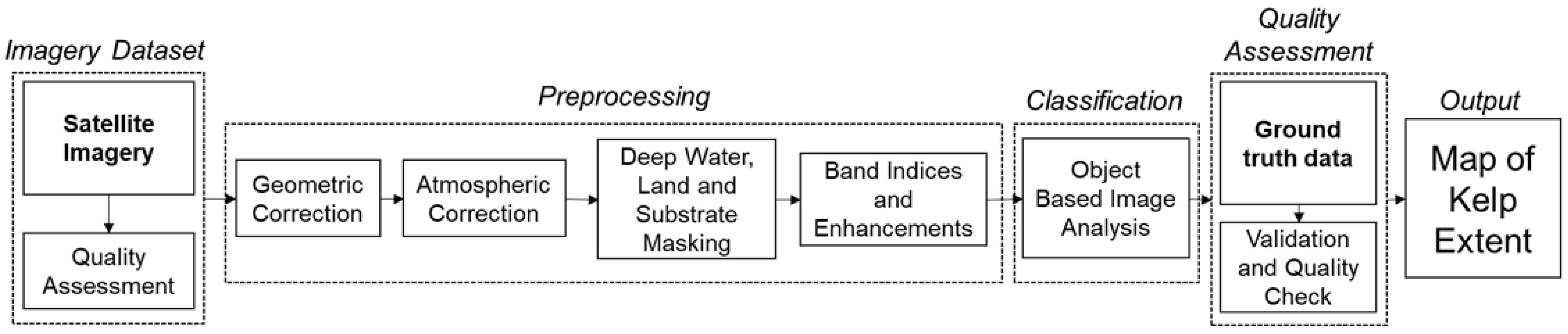
2.2. Methodological Framework

The framework is a workflow that allows researchers to compile robust temporal datasets of floating kelp canopy area through the evolution of medium- to high-resolution satellites. The workflow consists of four main steps, including: (1) imagery compilation and quality assessment; (2) preprocessing and enhancements; (3) object-oriented image classification; and (4) an accuracy assessment (Figure 2). To compare floating canopy area derived from multiple satellites, we analyzed kelp’s detectability at different spatial resolutions.

2.2.1. Step 1: Imagery Dataset

Archived high- to medium-resolution (0.5–60.0 m) multispectral satellite imagery was compiled from 20 satellite sensors spanning from 1973 to 2021 through diverse sources, including open data, private data sharing agreements, and commercial acquisition (Table 1). Archived imagery is not necessarily collected during optimal conditions for mapping, and therefore special consideration should be given to any factors that may lead to inaccurate maps of floating kelp forests, such as clouds, tidal height, glint, shadow, haze, water turbidity, waves, algal blooms and time of imagery acquisition [19,25,43,45,47]. To minimize possible inaccuracies, a set of criteria were developed, and images were visually assessed considering: glint, waves, shadows, clouds, the month and tidal height of acquisition. Each category was scored from 0 to 3, where the lower the score, the better the quality. For instance, the criteria for ideal conditions (score of 0) consisted of an acquisition time between June and October, a low tidal height (<3 m above lower low-water large tide chart datum) and the minimal presence (<5%) of glint, waves, shadow and cloud within the nearshore areas where floating kelp forests are found within the imagery [25,38]. Once combined, images showing suboptimal conditions for detection (overall criteria score ≥ 7) were removed from the dataset. Importantly, the quality score results should be framed within the context that more recent imagery is intrinsically more reliable for mapping floating kelp forests due to their higher spatial resolutions.

2.2.2. Step 2: Preprocessing

After selecting the optimal images for mapping, the following techniques were applied to reduce geometric and radiometric uncertainties and enhance the spectral signal of floating kelp to improve classification accuracies [25]. Geometric distortions occur in imagery due to errors during acquisition, such as variations in altitude, attitude, the velocity of the satellite, earth curvature, atmospheric refraction, and nonlinearities in the satellite path [44,67]. All selected images were checked for geometric distortions against the ESRI satellite base map in the WGS 1984 coordinate system, and those with distortions were georectified in ArcGIS using ground control points and a nearest neighbor interpolation [44,68]. However, where overlaps between imagery occurred, the overlapping images were georectified to the previous images to ensure the best match. The root mean squared error (RMSE) was calculated to evaluate the quality of the georectification, and a threshold of less than two pixels was deemed acceptable, except for the Landsat imagery, which was given an allowance of one pixel due to the coarser spatial resolution.
Following the georectification, images were evaluated for radiometric/atmospheric issues, which may impact the band indices used and, consequently, the imagery classification outputs [69,70]. When possible, we obtained atmospherically corrected images from suppliers (Table 1). For the other imagery, a simple approach considering a histogram shift determined by the Rayleigh scattering factor was applied [71], hereafter referred to as the Rayleigh correction. This approach considers that the scattering intensity is inversely proportional to the fourth power of the wavelength (λ−4), and assumes that the darkest pixels in an image, corresponding to shadowed or offshore deep-water areas, should have null reflectance; however, because of Rayleigh scattering, nonzero values are recorded [71]. To account for the Rayleigh scattering, these nonzero values are subtracted from the spectral signal of each specific satellite band, considering the spectral relationship between bands according to the Rayleigh factor (λ−4) [71]. The initial step is to define the lowest reflectance value in the blue band acquired from the darkest (lowest reflectance) pixels within the image (Bc), which is consequently subtracted from each pixel in the blue band. If no blue band was available (i.e., SPOT 4 and 5, Landsat-1 to 3), the value from the darkest pixels in the green band was divided in half to account for the lower proportion of Rayleigh scattering occurring and used in place of the blue Bc. Then, for each remaining visible band, the following equation is used to calculate the Rayleigh correction value (Rc):
R c = ( ( 1 / ( λ b 4 ) ( 1 / ( λ v i s 4 ) ) × B C ,
where λb represents the mean wavelength (nm) of the blue band, and λvis represents the mean wavelength (nm) of whichever visible band the equation is being used to calculate the correction for (e.g., 560 nm when correcting the green band of Geoeye-1). To ensure images were properly corrected, we evaluated the corrected reflectance of water and floating kelp for a subset of imagery from each sensor and compared them to the known reflectance for floating kelp and water from the literature [25,44,62].
Following the required corrections, images were subjected to: (i) a lowest tide land mask; (ii) a deep-water mask; and (iii) a soft substrate mask to eliminate areas where floating kelp forests are not found, and to minimize processing time and false positives. Vegetation and intertidal seaweed on land have a high near-infrared (NIR) reflectance compared to kelp [72,73], and therefore removing these features enhances the ability to digitally differentiate floating kelp from water through contrast enhancement [25]. We created the land mask using an object-based segmentation (Trimble eCognition Developer V8.64) on the imagery with the lowest tide. For each resolution of imagery used in this study, we added a buffer of one pixel to minimize land reflectance adjacency impacts from the shoreline. To eliminate any areas where floating kelp forests were unable to grow [74,75], a 20-m deep-water mask was created using a bathymetry dataset from the Canadian Hydrographic Service [38,46,76]. Lastly, we masked shallow-soft sediment bottom, which is uninhabitable to kelp [77], using overlapping areas defined as soft sediment in the BC Marine Conservation Analysis (BCMCA) benthic classes dataset [78] and the DFO bottom patch model [77].
The final task in the preprocessing workflow was to select the combination of bands, and band indices and/or band ratios, that perform best in the classification step. The normalized difference vegetation index (NDVI, i.e., the normalized difference between the reflectance of the near-infrared and red bands [79]) was used since it is commonly used to enhance floating kelp canopies in imagery from the Sentinel-2, Landsat and SPOT satellites [19,25,46,48,50,62,63,64,65,66] (Table 1). Additionally, for any imagery acquired by a sensor that had not been readily used for floating kelp forest detection in the literature, the M-statistic, a measure of class separability [80], was calculated for defining other possible band indices and ratios. A high M-statistic represents high separability between two classes with significant separation when M is larger than 1.0 [80,81]. For each sensor, we combined the two to three highest scoring band indices, or ratios, with the visible bands and visually assessed the combinations to choose which provided the best overall classification results (Table 1). The selected bands, band indices and ratios, were then linearly enhanced to maximize the spectral signal of floating kelp for the final input into the classification.

2.2.3. Step 3: Classification

An object-based image analysis (OBIA) was used based on the recommendation for classifying dense floating kelp forests [25]. The OBIA approach combined a multiresolution segmentation followed by a supervised nearest neighbor classification using the Trimble eCognition Developer (V8.64) software to classify floating kelp forests within the imagery. The OBIA classification offers several advantages over pixel-based classification methods. OBIA has shown better accuracy than pixel-based methods when compared across a range of spatial resolutions and ecosystems [82,83,84,85,86] and allows for the size of objects to be scaled, so that object size remains relatively constant across different resolutions [84]. As part of the eCognition software, OBIA allows for the definition of features beyond the pixel values of the input data, including the mean and standard deviation of object radiometry, object size and shape, and the spatial relationships of objects. This is not considered in pixel-based classification, thus increasing separability among classes and reducing the contribution of noise to the classification comparatively to pixel-based methods [87]. In the OBIA, the final enhanced bands, band indices and/or band ratios for each image were subjected to a multiresolution segmentation (Scale: Table 2; Shape: 0.3; Compactness: 0.5) to group similar pixels into objects. From those objects, training classes corresponding to floating kelp, submerged kelp/understory seaweed, water, glint/waves, cloud, shadow and shallow water, were defined using expert knowledge. Figure 3 shows examples of the most common classes used in the OBIA. Of note, not all classes were present in all imagery. In particular, some classes, such as glint/waves and submerged kelp/understory seaweed were indistinguishable in the medium-resolution satellite imagery. Because classes varied by image, the feature space optimization tool in the eCognition software was used to mathematically calculate the best number and combination of object features, such as the spatial, spectral and contextual information (e.g., the mean of bands/band indices, the standard deviation of bands/band indices, the maximum difference across all values of all bands/band indices), to separate classes based on training samples [88]. This tool compares features of different sample classes to find the optimal combination that produces the largest average minimum distance between samples, to be used when categorizing the remaining image objects into those given classes [88]. The ability of the feature space optimization tool chosen features to separate classes was evaluated based on the analysis of boxplots and three-axis scatter plots of the top three selected features for a subset of images. Following this evaluation, we performed a nearest neighbor classification, using the optimal features defined by the feature space optimization tool, to categorize the remaining image objects into their respective classes. Before validation, the outputs were visually subjected to a quality assessment using a knowledge-based approach where erroneous classifications were manually reclassified in ArcGIS. Lastly, for the validation step, the outputs of the classification were turned into two binary classes: floating kelp forests (1) and all other classes (0).

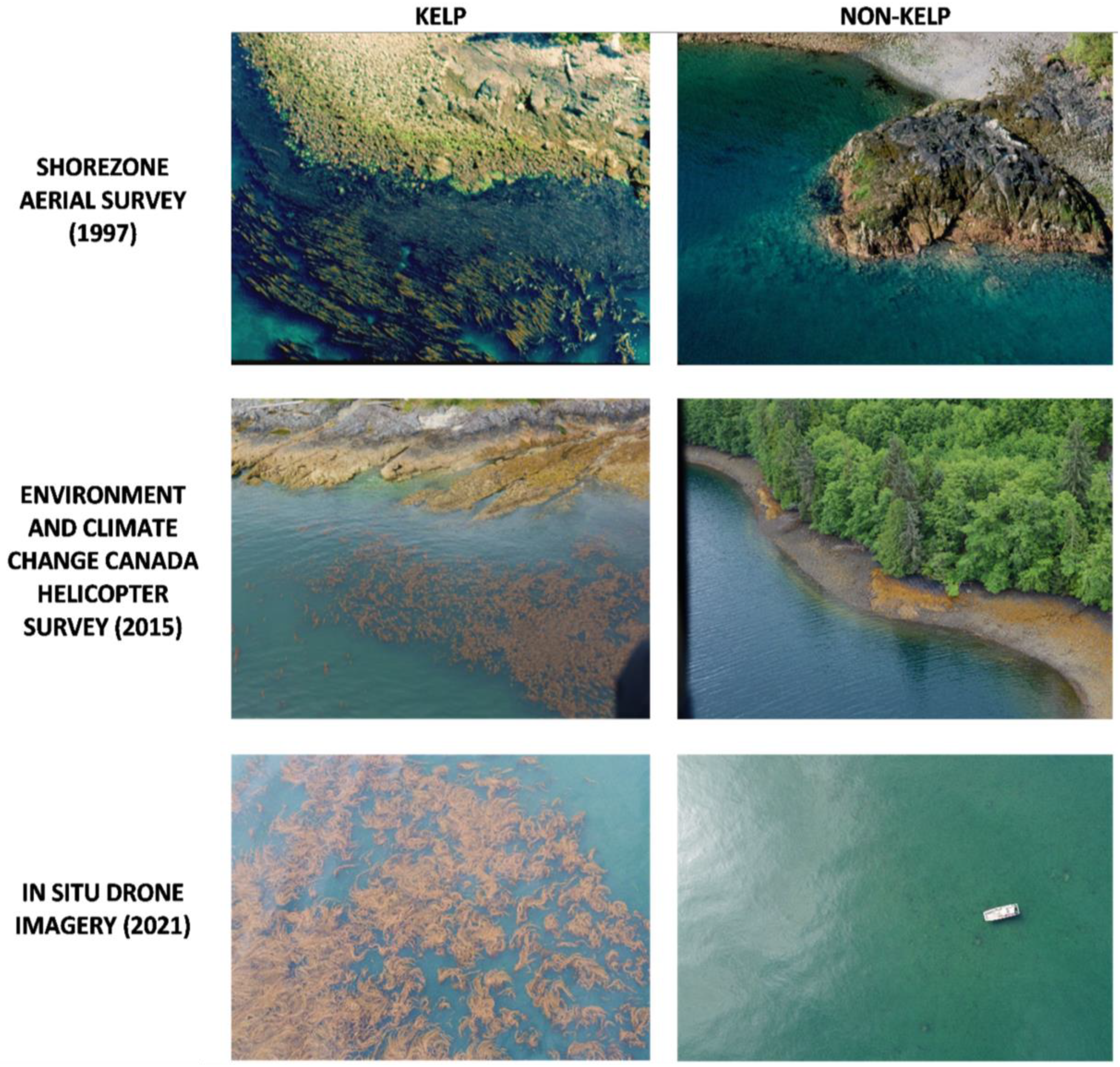
2.2.4. Step 4: Quality Assessment

For the classification validation, in situ kelp data and historical survey data for the region were compiled. Ideally, ground-truth data should be collected at the time of satellite imagery acquisition [25]. However, if no ground-truth data are available, other forms of data can be used, such as past surveys showing the location of floating kelp forests [38,50,89], or expert knowledge based on reflectance values [35]. For our dataset, we compiled two forms of validation data: (i) in situ and (ii) archived data (Figure 4). The in situ data, including drone images, photoquadrats (camera mounted above a 1 m quadrat lowered to the seafloor), above water oblique photos from a boat, and remotely operated underwater vehicle footage, were acquired in August 2021, a day after PlanetScope imagery acquisition. Archived surveys were obtained, comprised of oblique photos from an aerial survey performed by Environment and Climate Change Canada (ECCC) in 2015, multiple years of SCUBA surveys (1990, 1994, 2007, 2012, 2017) from the Department of Fisheries and Oceans Canada (DFO) [90] and kelp shoreline classifications from an aerial survey conducted in 1997 by ShoreZone. All validation data were combined into a dataset of spatial points and classified as either floating kelp present or absent. Specifically, the DFO Scuba surveys and ShoreZone data were simplified from species specific data (Macrocystis and Nereocystis) to presence and absence. For the archived aerial images from ECCC, a random subset of images was visually assessed for presence or absence. All validation data were compared to the classification produced from imagery in the matching year to produce measurements of accuracy corresponding to users’, producers’ and global accuracy, meaning errors of commission (false-positives), omission (false-negatives) and overall accuracy [91]. No archived validation data were available during the years of acquisition for the three highest resolution satellites, so in order to validate products from the QuickBird-2, Geoeye-1 and Worldview-2 satellites, the ECCC oblique photos were used with the assumption that some errors would be associated with yearly variability.

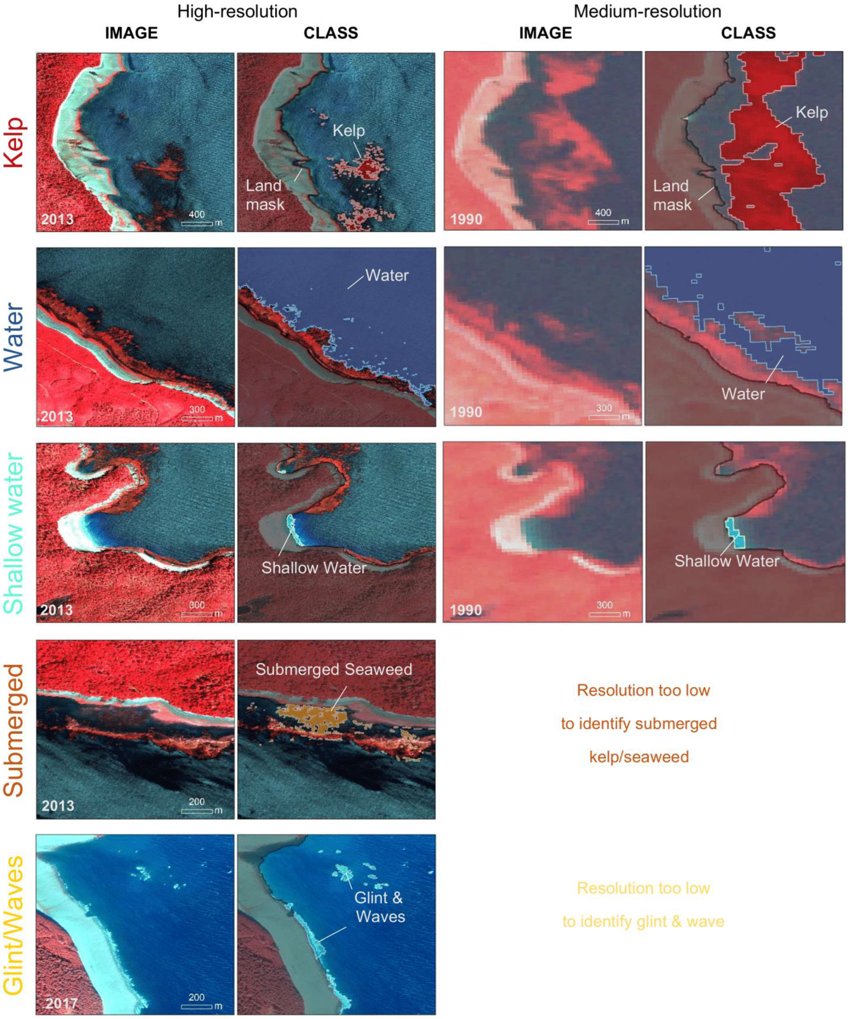
2.2.5. Resolution Analysis

Here, we evaluate the impact of spatial resolution on the detectability of floating kelp forests in satellite imagery at different scales. This analysis allowed us to define an independent variable (ocean floor slope) to be used as an indicator of kelp forest size, highlighting areas of uncertainty. The following steps were adopted in this analysis:
Step 1: Images from QuickBird (2.6 m), RapidEye (5.0 m) and Sentinel-2 (10.0 m), with their original spatial resolutions, were resampled using bilinear interpolation to the different resolutions matching the satellite database (6.0 m, 10.0 m, 20.0 m, 30.0 m, 60.0 m; Table 1) following [92,93]. Sentinel-2 was included in the analysis to address possible interpolation errors [94] associated with resampling high-resolution imagery from QuickBird-2 and RapidEye to 20.0 m, 30.0 m and 60.0 m resolutions. The original and resampled images were classified using the OBIA method described in Section 2.2.2 and Section 2.2.3. To ensure that images from the same sensor remained comparable, we used the same areas to train the classifier for each set of down-sampled images. After the classification of the resampled images, the overall detectability across the study region was measured as the total amount of floating canopy area (m2) detected in the downgraded resolution, divided by the total floating canopy area (m2) detected in the original image, and presented as the percentage of floating canopy area.
Step 2: A 1 km segment-based approach was used as the areal unit to evaluate the impact of resolution (see Figure 5 for the delineation of segments). Due to the complex bathymetry and presence of large offshore and nearshore floating kelp forests in our study area, ocean floor slope was used to delineate these segments, as adapted from [95]. To achieve segments that could extend kilometers offshore, segments were created in two categories, along the shoreline (ocean floor slope greater than 3%) and out across the low slope areas extending offshore (ocean floor slope of less than or equal to 3%), using 20 m bathymetry data from CHS [76]. These ocean floor slope categories were only used to construct the segments and were not used in further analyses.
Step 3: Ocean floor bathymetry often limits the size of kelp forests by reducing the available area to grow [46,96]; therefore, we assume it can be used as a proxy for kelp forest size. For example, in high slope areas, the bottom quickly becomes too deep, limiting the availability of light needed for kelp to establish and grow. In these conditions kelp only grows in narrow fringing forests, which are more difficult to detect in satellite imagery. Consequently, ocean floor slope was used to define areas where we would expect larger inaccuracies of the classification at different resolutions. However, first we tested the assumption that high slope areas support small fringing kelp forests [46].
For this, the relationship between ocean floor slope and kelp forest size was explored (classified from the original QuickBird-2, RapidEye and Sentinel-2 images and measured in m2). For each segment, we defined the mean ocean floor slope based on the 20 m bathymetry data from CHS [70], where a single kelp ‘forest’ was defined as a continuous patch of attached floating kelp where kelp objects in the classification were connected. Based on the relationship of floating kelp forest size and ocean floor slope, we divided the segments into two broad categories: low–mid slope areas (0–11.3%), which support large and small kelp forests, and high slope areas (11.4–37.0%), which support only small kelp forests. Next, floating canopy area percentage was compared between the two slope categories.

3. Results

3.1. Imagery Quality Assessment
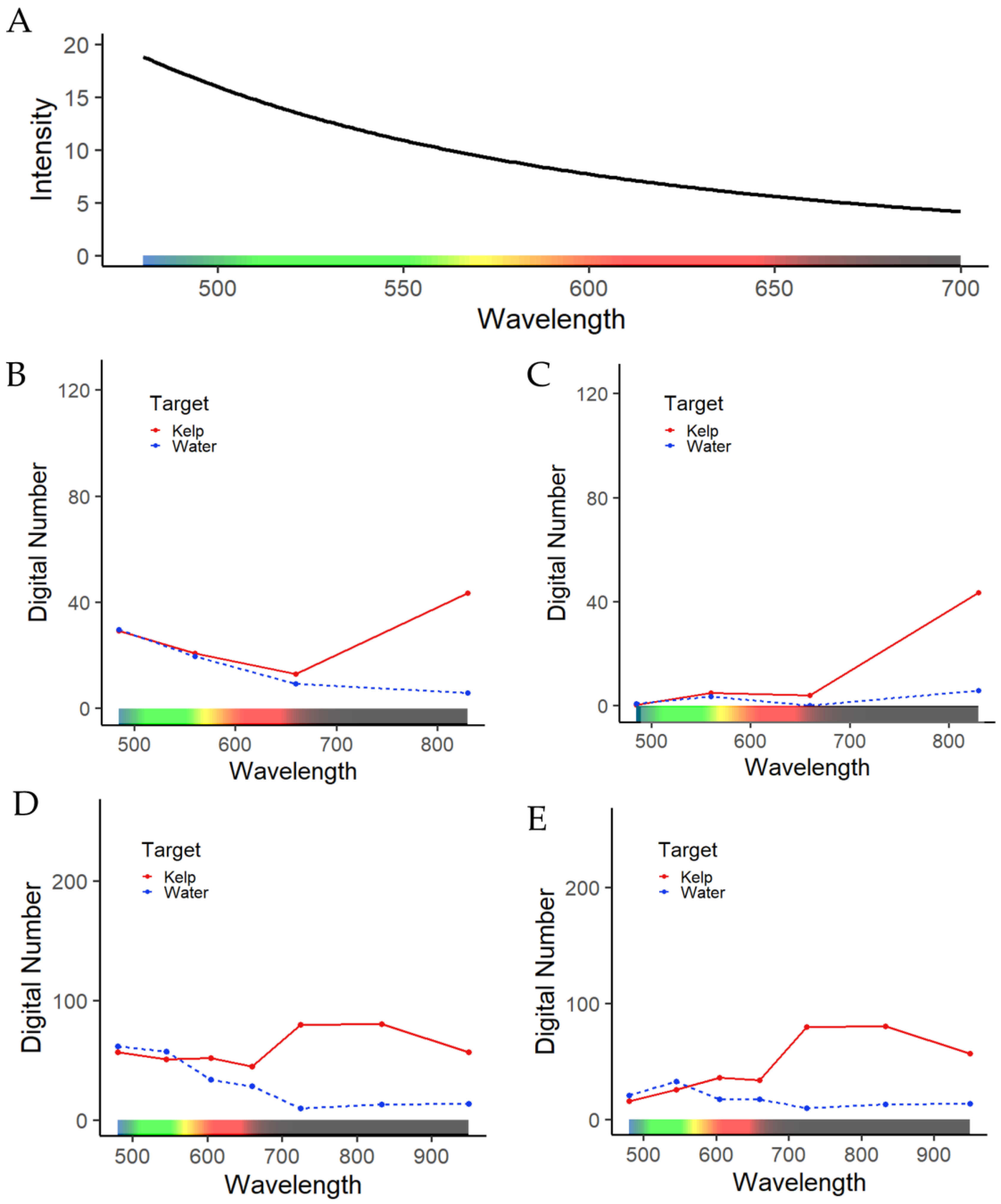
Out of hundreds of archived images examined across many different sources (Table 1), a total of 52 images (from 1973 to 2021) were selected after the quality assessment step. No good-quality images were found for a total of 12 years, including 1975, 1978–1981, 1983, 1987, 1993, 1995, 1996, 2003 and 2004. Landsat was the only freely available satellite imagery provider before 2004 and thus the preferred choice for imagery; in particular, Landsat-7’s scan line corrector failure in 2003 [97] led to no available images for 2003 and 2004. For years following 2005, the preferential choice was for high-resolution imagery (2.0–20.0 m). Imagery from a single Spot 4 image (20.0 m) to numerous images from Sentinel-2 (10.0 m), QuickBird-2 (2.6 m), Geoeye-1 (1.8 m), Worldview (1.2 m and 1.8 m), PlanetScope (3.0 m resampled from 3.7 m) and RapidEye (5.0 m) satellites were compiled. In addition to the high-resolution satellite imagery, we included a single nadir RBG aerial image (0.5 m spatial resolution) from the Canadian Hydrographic Service in the dataset because of the lack of good-quality high-resolution satellite imagery in 2007.
The 52 archived images selected through the criteria were acquired in various conditions, leading to a range in quality scores (Table 3). The largest proportion of imagery (46%) were acquired during ‘optimal’ conditions for floating kelp forest mapping, followed by the second largest proportion (37%) acquired during ‘good’ conditions. Together, the ‘good’ and ‘optimal’ imagery account for 83% of the total imagery. Among the defined criterion, more often, high tides or the presence of glint and cloud in imagery led to lower scores than waves and haze (Table 3). Notably, in some years, no optimal low tide (<3 m above chart datum) imagery was available because of the high tidal exchange that occurs in Haida Gwaii (up to 7.8 m above chart datum) [98], leading to 33% of images ranked in the lowest category for tides (5.0 to 6.0 m). These images were still included in the time series dataset because floating kelp forests were readily visible upon inspection.

3.2. Preprocessing

Considering the selected imagery used for further analysis, a total of six images needed geometric correction: one from Landsat-1, and all imagery from QuickBird-2 and Geoeye-1, resulting in a RMSE within the two pixel threshold (average RMSE: QuickBird-2: 4.49 m, Geoeye-1:3.61 m, Landsat-1: 16.48 m). For the next step, Rayleigh correction was applied to imagery from Landsat-1–3, QuickBird-2, SPOT 5–7 and Geoeye-1; images acquired by the other sensors (Sentinel-2, RapidEye, PlanetScope and Landsat-5) were provided in atmospherically corrected products. After Rayleigh correction, our results showed that compared to the original values, floating kelp and dark water pixels in the blue band were reduced to zero or just slightly above, in the green band, pixels values decreased by approximately half, and by approximately a third in the red band (Figure 6). This conforms with the shape of kelp spectra and water spectra from in situ hyperspectral measurements of floating kelp and water, in literature [25,44,62].
After geometric and Rayleigh corrections, the different spectral indices were evaluated based on the M-statistics. Among the available spectral indices, the M-statistic results showed different optimal indices for the different satellites (Table 4). For Geoeye-1 and QuickBird-2, a normalized vegetation index with the green band (G-NDVI) instead of the red band had the highest separability (>1.44). Meanwhile, for PlanetScope imagery, a simple ratio combination of the near-infrared and green bands showed the highest separability (>11.34). Lastly, for satellites that included a red-edge band, RapidEye and Worldview, a simple band ratio of red-edge over green (>1.69), and red-edge over yellow (>2.72), was best at separating kelp from water, respectively. The statistically selected indices and bands were used as the input data for the object-oriented classification.

3.3. Classification & Accuracy Assessment

Here, the results are presented according to the order of the various decision processes for the classification and validation. In an object-oriented classification approach, after the initial segmentation step (see Methodological Framework Step 3: Classification), the feature space optimization tool of eCognition defined the combination of object features that best differentiate classes. Specifically, the feature space optimization function defines the best combination of object features that gives the highest possible separability between classes, as illustrated by the example of features chosen to classify a QuickBird-2 image (Figure 7). In this particular case, the feature space optimization tool chose the standard deviation of G-NDVI, the mean G-NDVI, and the maximum difference between all bands and band indices to differentiate floating kelp canopy from submerged seaweed/kelp, glint/waves and water sample classes. Mean G-NDVI alone can differentiate kelp from all other classes present in the image. However, the feature space optimization chose both the standard deviation of G-NDVI and the maximum difference between all bands and band indices because, when combined, they can differentiate among all classes (Figure 7). For the majority of the dataset, the feature space optimization tool selected between three and 10 features depending on the image, with, generally, the mean of the red-edge band (when available), the mean of the near-infrared band and/or the mean of the band indices selected.
After selecting the optimal features, we ran the classification according to the nearest neighbor algorithm, followed by an evaluation of the classification results, considering user, producer, and global accuracies (Table 5). The overall global accuracy for all sensors ranged from 88% to 94% (Table 5). Generally, producers’ and users’ accuracy for kelp was high (from 83% to 96% and from 90% to 100%, respectively; Figure 8C,D). Producers’ accuracy for non-kelp classes were also high (from 89% to 100%). The lowest scores occurred within the non-kelp users’ accuracy (from 64% to 100%) with errors occurring where floating kelp was misclassified as water (see example in Figure 8A,B). Lastly, we found no apparent differences when comparing the accuracy assessments that used concurrent and non-concurrent validation data for QuickBird-2, Geoeye-1 and Worldview-2 (Table 5).
We used, on average, 124 validation points (85 kelp points and 39 non-kelp points), except for with the classification of RapidEye and the aerial imagery. For these, only nine validation data points were available for each, and thus even though high accuracy was achieved, caution about the results is recommended. The lowest resolution satellite, Landsat-5 (30.0 m), included in the validation, had similar accuracy to the higher-resolution satellites (Table 5); however, it produced the lowest measure of users’ accuracy for non-kelp targets (64%). Upon inspection, smaller thin fringing forests in steep nearshore areas were misclassified as water or omitted due to the lowest tide land mask’s coarse resolution.

3.4. Resolution Analysis

Figure 9 illustrates the relationship between pixel size and the mixing of the spectral signature of different features within a pixel. Specifically, within a pixel resolution (for instance, 30.0 by 30.0 m for Landsat-5), the kelp spectral signature is averaged with the spectral signature of other classes in close proximity (e.g., water), decreasing the ability to accurately map floating kelp forests as pixel size increases. In particular, as resolution decreases, floating kelp and water spectrum are mixed, and the reflectance in the near-infrared wavelengths decrease (Figure 9G). At the sample location shown in Figure 9, the object-based classification can no longer differentiate the floating kelp signal from water at 60.0 m (Figure 9G).
Pixel mixing decreases the ability to correctly classify floating kelp when using medium-resolution imagery. We show that at downgraded resolution, images generally produced a floating canopy area within 9% of their image’s original kelp forest area (Figure 10). For instance, at 6.0 m resolution, the mapped floating kelp canopy area is 93%, i.e., 7% lower than the mapped area at the original 2.6 m resolution. This can be assumed up to a certain downgraded resolution because the further an image is downgraded away from its original resolution, the more likely artifacts or errors from the interpolation methods may occur, such as blurring and edge halos [94]. This possible issue is minimized by avoiding data analysis of downgraded high- to medium-resolution, and instead, considering a downgraded Sentinel-2 image from 10.0 m (SE10) to 20.0 m, 30.0 m and 60.0 m (SE20, SE30 and SE60, respectively). In this case, the results show that the floating kelp canopy area remained almost unchanged when downgrading the medium-resolution Sentinel-2 image from 10.0 m to 20.0 m, 30.0 m and 60.0 m (Figure 10C).
Figure 11 shows the relationship between floating kelp forest size (produced from the three original images) and ocean floor slope. Generally, areas of low–mid slope (0–11.3%) were associated with both small (<17,000 m2) and large kelp forests (≥17,000 m2), whereas high slope (>11.4%) areas were only associated with small fringing kelp forests (<17,000 m2). The low–mid slope areas exhibited a lower percent difference (within 7%) of floating kelp forest area between the various imagery resolutions than the high slope areas (up to 50%) overall (Figure 12). In particular, the differences in floating canopy area in high slope regions were much more pronounced in the downgraded medium-resolution imagery (SE20, SE30 and SE60) than the high-resolution imagery (QB6, QB10, RE6 and RE10). These results allowed us to restrict the use of medium-resolution imagery to map floating kelp forests only in areas of mid–low slope, i.e., imagery resolution between 20.0 and 60.0 m is not recommended for high slope areas where fringing small kelp forests dominantly occur.

4. Discussion

With advances in remote sensing technology, opportunities to map and monitor important ecosystems across large scales through time are increasing. The Landsat series offers the best tool to map floating kelp forests at a single resolution (30.0 m) back through time [13,19,46,62,63,99]. However, the ability to use medium-resolution imagery to accurately map changes in floating kelp canopy area through time remains difficult in regions with small fringing kelp forests, such as the Pacific Coast of Canada and Oregon [46,52]. Here, we developed a framework combining standardized practices and adaptable methods to produce a long time series of accurate maps of floating kelp forests from satellite imagery acquired at various spatial resolutions. We show that the ability to map floating kelp forests at different imagery resolutions can vary spatially based on ocean floor slope, and thus this metric can be used to highlight areas of uncertainty. Herein, we make a case for the workflow, discuss the impact of spatial resolution on kelp detection, summarize recommendations for researchers when using the multi-satellite mapping framework (Table 6) and more broadly consider the limitations and applications of the research.

4.1. Methodological Framework: Standardization and Adaptability

In remote sensing, Earth observation satellite data has become readily available, and users often face confusion when trying to determine which satellites to use to produce the best results for their given application [100]. In this paper, we highlighted some of the most well-known sensors for mapping floating kelp forests, such as the Landsat, SPOT and Sentinel-2 satellites (e.g., [19,46,62,65]), while also presenting some new cost-effective high-resolution options such as imagery from RapidEye, Worldview and PlanetScope satellites, which add valuable data into the kelp mapping field with their coverage since 2008, 2009 and 2018, respectively. In addition to the choice of satellites, having a specific set of criteria when choosing what images to use is crucial in minimizing the time and cost associated with building a time series (Table 6) [38,100,101]. We demonstrated one possible set of criteria that can be used to minimize errors associated with environmental conditions and the timing of satellite imagery acquisition. Of note, the criterion should always be selected based on the specific areas of interest. In particular, other factors that could lead to the erroneous classification of floating kelp forests in satellite imagery are land adjacency effects, high currents independent from tides, water turbidity and the presence of algal blooms [47]. Our analysis did not consider these because they were largely absent in our study region. However, in our case, clouds and higher amplitude tides often limited the availability of good quality images. As such, some mid- to high-tide images (3.0–5.0 m above chart datum) were included, based on a visual assessment of the imagery. A loss of floating canopy area up to 42% when comparing a 2.0 m tidal height difference was found on the Central Coast of BC [46]. In California, where Macrocystis kelp forms large offshore forests similar to those found within the study area, increases in tidal height of 1 m in UAV imagery reduced the floating canopy area from 15% to 30%, but was site dependent [102]. However, little to no difference was detected in Landsat satellite-derived kelp biomass measurements across a 2.0 m tidal difference, likely related to the coarse resolution [19,50]. Consequentially, researchers should be aware of the impact that tides can have on detection when determining their tide criterion and using this framework for time series analyses. The impact of tides can be site, species, density and kelp forest size dependent [102,103]. Upon visual comparison we found no major difference between tidal heights used in this study; however, more analyses are needed to understand and quantify the impact of tides in this region.
Once a good quality imagery database is created, users are faced with many inconsistent and complex approaches to correct systematic errors, such as atmospheric attenuation and geometric distortions in imagery [25,104]. In order to keep the workflow streamlined and easy to use, we propose a simple geometric and atmospheric correction method that can be applied to imagery from various sensors (Table 6). For georectification, we found that a simple first-order polynomial shift, which considers systematic and random distortions in images [44,67,105], properly addressed any geometric distortions present. There are numerous atmospheric correction methods that range from simple techniques like the Rayleigh correction method [63] to the more complex algorithms that need supplemental data, including atmospheric models and, ideally, in situ measurements [106,107]. Other researchers, for instance, have effectively used models such as the Fast line-of-sight Atmospheric Analysis of Hypercubes (FLAASH) [35] and the Atmospheric and Topographic Correction (ATCOR) [46]. Nonetheless, these methods can often under- or overcorrect values when parameters are not adequately chosen, making it challenging for non-remote sensing experts to use, and problematic when applied over large bodies of water [108,109,110]. When possible, imagery should be downloaded as already corrected products, such as in [52,53,62,65]. For example, the United States Geological Survey (USGS) provides Landsat Analysis Ready Data (ARD) products [111] and the Planet provides Surface Reflectance (SR) products [112]. However, when these products are not available, adhering to a simple method that only requires within-image information is recommended to prevent errors related to inconsistent methods or data input. We found that the adopted Rayleigh correction method resulted in similar floating kelp and water spectra as those from the literature [25,44,62]. More importantly, the shape of the floating kelp and water spectra from the corrected images were akin to those of the atmospherically corrected products.
Numerous band ratios and vegetative indices have been used to enhance floating kelp forests in satellite imagery [25]. Most notably, NDVI, which was initially used to detect healthy land vegetation [113], has been co-opted for floating kelp forests [19,25,46,48,50,52,53,63,114]. Based on the literature, NDVI has been effectively applied to Sentinel-2, Landsat and SPOT satellite imagery to differentiate kelp from other classes. Alternatively, based on M-statistic analysis, and similar to [25], we found that the NDVI with the green band (G-NDVI) instead of the red band performed better, most likely because less noise was visible in the green band than in the red band. Additionally, indices that included the red-edge band outperformed other indices, likely associated with the ability to detect slightly deeper kelp better than the near-infrared band [115]. Considering these factors, within an image pixel, there is likely a spectral signal mixture of submerged and floating kelp canopy with water; consequently, users should consider that the red-edge indices may produce a higher reflectance signal or slightly more kelp area than nonred-edge indices, depending on the properties of the kelp forest (percentage submerged, depth, size, density, species, object size). Although different band indices were chosen in our analysis, the overall accuracy of the kelp maps produced remained high across all satellites regardless of chosen index, indicating the viability of using different band indices to enhance the detection of floating kelp forests.
Among the many different forms of classification, a commonly used method, the Multiple Endmember Spectral Mixture Analysis (MESMA), has been effectively used for mapping kelp forests in Landsat imagery. The MESMA is a pixel-based approach, which linearly models the amount of kelp and seawater in each pixel using one kelp pixel endmember and multiple water pixel endmembers [19,19,50,62,99,116,117]. In comparison, the OBIA approach presented herein and first used by [25,38] to map kelp forests, is based on clustering pixels into objects before the classification. The advantages of using the OBIA approach proposed in this framework are related to less computational power, less consideration of imagery noise commonly found in pixel-based classifications, the ability to mimic the visual interpretation of features in an image, and the ability to scale object sizes to remain similar across different resolution imagery [25,83,84,84,85,118,119]. Most importantly, the feature space optimization tool allows for the classification to be optimized on a per image basis. With an OBIA approach, single kelp plants are not being detected, but the aggregates of plants floating at the surface, with the inclusion or some submerged kelp and water gaps between patches, depending on the size of objects selected by the user. This gives users the ability to define the best object size based on forests in their region and the resolution of imagery used. Additionally, when users are trying to detect very small and sparse fringing forests in high-resolution imagery, that result in single pixels needing to be classified as kelp, a pixel-based classification has shown to outperform OBIA [25]. In this case, users should be cognizant of the limitations of OBIA and should test the performance of pixel-based methods described in [25].
Across all sensors, the multi-satellite mapping framework resulted in high overall global accuracy (from 88% to 94%) when compared to the range (from 59% to 94%) documented in the literature [25,38,46,52,66]. It is important to note that different sources of validation data were used to evaluate the classification results, including field observations concurrent with imagery acquisition, data acquired from airplane and SCUBA surveys, matched for the same year, and some not matching the same year. However, for using all the different data sources, expert knowledge was always embedded prior to the accuracy assessment to minimize the use of erroneous classification outputs when comparing with validation data. Generally, the errors of omission and commission showed that most errors occurred at medium-resolutions where sparse, and narrow fringing forests along steep shorelines were misclassified as water or omitted due to the coarse resolution low water mask, similar to [46]. This indicates that the relationship between imagery spatial resolution and floating canopy area has to be considered to highlight mapped areas with high uncertainties.

4.2. The Impact of Resolution and Drawing Appropriate Conclusions

The framework presented here incorporated the analysis of a large range of satellite imagery with spatial resolutions ranging from 2.5 to 60.0 m (except for the one aerial image with a resolution of 0.5 m). Generally, although the imagery resolutions differed by one order of magnitude, the mapped floating canopy area at the regional level did not largely differ among resolutions. However, at a finer spatial scale, we found that the floating canopy area mapped in high slope areas (associated with fringing kelp forests) were more impacted at coarser resolutions, indicating that these areas are prone to higher classification errors. As such, we propose the addition of a new parameter, ocean floor slope, to define the limitations of mapping floating kelp forests from different resolution imagery. Particularly, the comparison between floating kelp forest size and slope showed that high slope areas support small kelp forests, leading to more uncertainty when mapping with medium-resolution imagery (up to 50%). Based on these factors, we suggest that regions with slopes higher than 11.4% should either be mapped only with the high-resolution imagery or excluded from comparisons between high-resolution and medium-resolution imagery (Table 6). Additionally, for the time series of floating kelp forest change, we recommend that users consider that a certain percentage of differences among years can be attributed to errors due to resolution, and not be attributed to true changes in floating canopy area. Within our region, we suggest that changes up to 7% (with high slope areas removed from the analysis) be taken into consideration when comparing area from imagery at different resolutions (Table 6).

4.3. The Challenges and Broad Applications of the Methodological Framework

A few challenges and limitations remain when using this proposed framework. Unfortunately, the remote sensing of kelp canopies in this framework are currently limited to those floating on or close to the surface, due to water’s high-absorption of the near-infrared signal [115]. The detection of subsurface kelp forest canopy from aerial and satellite imagery remains difficult, is limited to shallow depths, generally necessitates clear waters and often requires the use of high-resolution imagery or hyperspectral data [66,120,121,122]. More work would be needed to expand these methods to subsurface kelp forests. Additionally, environmental impacts (e.g., tides and currents) are challenging to isolate because they largely differ based on location, species type, density and the time of imagery acquisition. We were able to minimize the impact that different environmental conditions have on imagery through criteria; however, we were unable to quantify or create correction factors for the impact of tides or currents. Of note, given our goal to produce highly accurate floating kelp forest maps, the approach suggested here is a supervised classification method and needs some expert knowledge to determine good training samples for the classifier in any given area. Moreover, when using the multi-satellite mapping framework, researchers should consider the species and density of kelp forests present within their region. In our case, floating kelp forests were generally dense, regardless of the forest size and species, thus conforming with the presented framework. For other regions where sparse kelp forests dominate or areas containing solely Nereocystis kelp forests, special attention should be given to the detection limits at different resolutions, the use of OBIA versus pixel-based classifications for very small sparse forests [25] and the ocean floor slope threshold.
The spatial resolution analysis and subsequent recommendations were conducted with rigorous methodological criteria; however, the analysis was limited to samples of imagery from three satellites. We acknowledge that the sample size is limited, and other satellite-associated variables beyond spatial resolution, including spectral resolution, signal-to-noise ratio, and satellite vicarious calibration, also play a role in detectability [25,123,124]. However, the resolution analysis allows for a conservative approach when drawing conclusions from the time series of floating kelp forests. Additional research in the future may include defining correction factors, similar to the tidal correction factor applied by [62], to minimize the effects of the different spatial resolutions. For this, we recommend multiple replicates of comparisons between satellite images collected at different spatial resolutions in similar conditions over the same location, within a short time frame. Furthermore, it is important to note that our unit of analysis was ~1 km segments. In the literature, the size of segments for kelp time series analyses vary substantially (e.g., 100 m in [38], 8 km in [43] and 1 km in [125]), and as such, special consideration should be given to the scale of future analyses. We advise that further explorations of the resolutions’ impact on kelp detectability be made if the unit of analysis (segments length) significantly differs from the 1 km segment size presented in this study.
Many methods exist to detect floating kelp forests from satellite imagery; however, most focus on compiling a time series using a single type of sensor, which can limit either the spatial resolution of imagery available (i.e., 30.0 m Landsat imagery from 1984 onwards), or with the use of high-resolution satellite imagery the length of the time. The MESMA approach, used with Landsat imagery from 1984 onwards to detect large offshore forests of kelp in California [19,50,62,117], has been used to map Macrocystis in the southernmost part of Argentina [108] and Nereocystis off the coast of Northern California [91] and Oregon [52]. However, when this approach was used to map kelp forests on the Central Coast of BC, between 28% and 75% of kelp that was present in the shoreline areas was missed due to the medium-resolution of the Landsat imagery [43]. Recently, a similar method using 10.0 m Sentinel-2 data was created [65], and although this method uses higher-resolution imagery, the Sentinel-2 data repository only dates back to 2015. In contrast, the methodology presented here enables trends to be understood with high-resolution data back to the early 2000s, and medium-resolution data back to the 1970s. The methods proposed by [25,46,50,65], and the one shown here, when integrated with the growing availability of higher-resolution imagery such as the Planetscope satellite series (available since 2018), will streamline the monitoring of floating kelp forests into the future. It will also continue to allow scientists to better understand large-scale trends in floating kelp forests in a time of unprecedented kelp forest loss, such as those documented in California [117,126], Baja California [12], Japan [127,128], Australia [9,10,129,130,131,132], Oman [133], Norway [134], Spain [135,136], Chile [137] and the Atlantic Coast of Canada [11].

5. Conclusions

Globally, threats to kelp forests are on the rise; however, locally, kelp forests show highly variable patterns of change [1,3]. This study highlights that with the advancement in Earth observation satellite technology, archived satellite imagery can be leveraged for the monitoring of crucial floating kelp forest ecosystems using medium-resolution imagery from the 1970s onwards, and more recently, using high-resolution imagery from the early 2000s onwards. The multi-satellite mapping framework allows for the creation of a floating kelp canopy area time series using medium- to high-resolution satellite imagery through standardized practices (i.e., the image quality criteria, geometric and Rayleigh correction) and adaptable image-to-image methods (i.e., band index/ratio selection and OBIA). We acknowledge that differing resolutions have an impact on kelp detection, and that when using this framework we suggest using ocean floor slope (removing areas of slope > 11.4%) as a metric to highlight areas of uncertainty in kelp detectability. Creating these long time series of floating kelp forests using the framework can facilitate the monitoring and protection of these important nearshore habitats from emerging threats. Additionally, when coupled with environmental driver data and/or climate prediction modelling, it can highlight the regions of risk and resilience of floating kelp forests globally.

Author Contributions

L.G., M.C. and M.H.-L. designed the methodological framework; L.G. carried out the compilation, the processing of data and the writing of the manuscript with guidance from S.B.S., M.C. and M.H.-L.; P.W. facilitated the provision of some of the high-resolution satellite imagery and provided revisions on the manuscript. All authors have read and agreed to the published version of the manuscript.

Funding

During this research L.G. was supported through a MITACS Accelerate internship with the Hakai Institute, as well as M.C.’s NSERC-DG.

Data Availability Statement

Data are available for research purposes upon request to the authors’ institutions.

Acknowledgments

We thank the Hakai Institute for partially funding this work, as well as the Canadian Hydrographic Service, Transport Canada, the Department of Fisheries and Oceans Canada (in particular Joanne Lessard), Environment and Climate Change Canada, and ShoreZone, for providing satellite data and ground-truth data. A special thanks to Lynn Lee with Parks Canada and Stuart Crawford with the Council of the Haida Nation for assistance with field equipment in Haida Gwaii.

Conflicts of Interest

The authors declare no conflict of interest.

References

  1. Wernberg, T.; Krumhansl, K.; Filbee-Dexter, K.; Pedersen, M.F. Chapter 3—Status and Trends for the World’s Kelp Forests. In World Seas: An Environmental Evaluation, 2nd ed.; Sheppard, C., Ed.; Academic Press: Cambridge, MA, USA, 2019; pp. 27–78. ISBN 978-0-12-805052-1. [Google Scholar]
  2. Jayathilake, D.R.M.; Costello, M.J. Version 2 of the World Map of Laminarian Kelp Benefits from More Arctic Data and Makes It the Largest Marine Biome. Biological Conservation 2021, 257, 109099. [Google Scholar] [CrossRef]
  3. Bolton, J.J. The Biogeography of Kelps (Laminariales, Phaeophyceae): A Global Analysis with New Insights from Recent Advances in Molecular Phylogenetics. Helgol Mar Res 2010, 64, 263–279. [Google Scholar] [CrossRef] [Green Version]
  4. Johnson, S.W.; Murphy, M.L.; Csepp, D.J.; Harris, P.M.; Thedinga, J.F. A Survey of Fish Assemblages in Eelgrass and Kelp Habitats of Southeastern Alaska; U.S Department of Commerce: Washington, DC, USA, 2003; p. 48. [Google Scholar]
  5. Krumhansl, K.A.; Okamoto, D.K.; Rassweiler, A.; Novak, M.; Bolton, J.J.; Cavanaugh, K.C.; Connell, S.D.; Johnson, C.R.; Konar, B.; Ling, S.D.; et al. Global Patterns of Kelp Forest Change over the Past Half-Century. Proc Natl Acad Sci USA 2016, 113, 13785–13790. [Google Scholar] [CrossRef] [PubMed] [Green Version]
  6. Filbee-Dexter, K.; Wernberg, T. Rise of Turfs: A New Battlefront for Globally Declining Kelp Forests. BioScience 2018, 68, 64–76. [Google Scholar] [CrossRef] [Green Version]
  7. Eger, A.; Marzinelli, E.; Baes, R.; Blain, C.; Blamey, L.; Carnell, P.; Choi, C.G.; Hessing-Lewis, M.; Kim, K.Y.; Lorda, J.; et al. The Economic Value of Fisheries, Blue Carbon, and Nutrient Cycling in Global Marine Forests. EcoEvoRxiv 2021. [Google Scholar] [CrossRef]
  8. Bennion, M.; Fisher, J.; Yesson, C.; Brodie, J. Remote Sensing of Kelp (Laminariales, Ochrophyta): Monitoring Tools and Implications for Wild Harvesting. Rev. Fish. Sci. Aquac. 2019, 27, 127–141. [Google Scholar] [CrossRef]
  9. Wernberg, T.; Smale, D.A.; Tuya, F.; Thomsen, M.S.; Langlois, T.J.; de Bettignies, T.; Bennett, S.; Rousseaux, C.S. An Extreme Climatic Event Alters Marine Ecosystem Structure in a Global Biodiversity Hotspot. Nat. Clim. Change 2013, 3, 78–82. [Google Scholar] [CrossRef]
  10. Wernberg, T.; Bennett, S.; Babcock, R.C.; de Bettignies, T.; Cure, K.; Depczynski, M.; Dufois, F.; Fromont, J.; Fulton, C.J.; Hovey, R.K.; et al. Climate-Driven Regime Shift of a Temperate Marine Ecosystem. Science 2016, 353, 169–172. [Google Scholar] [CrossRef] [Green Version]
  11. Filbee-Dexter, K.; Feehan, C.; Scheibling, R. Large-Scale Degradation of a Kelp Ecosystem in an Ocean Warming Hotspot. Mar. Ecol. Prog. Ser. 2016, 543, 141–152. [Google Scholar] [CrossRef] [Green Version]
  12. Arafeh-Dalmau, N.; Montaño-Moctezuma, G.; Martínez, J.A.; Beas-Luna, R.; Schoeman, D.S.; Torres-Moye, G. Extreme Marine Heatwaves Alter Kelp Forest Community Near Its Equatorward Distribution Limit. Front. Mar. Sci. 2019, 6, 499. [Google Scholar] [CrossRef]
  13. Cavanaugh, K.C.; Reed, D.C.; Bell, T.W.; Castorani, M.C.N.; Beas-Luna, R. Spatial Variability in the Resistance and Resilience of Giant Kelp in Southern and Baja California to a Multiyear Heatwave. Front. Mar. Sci. 2019, 6, 413. [Google Scholar] [CrossRef] [Green Version]
  14. Smale, D.A. Impacts of Ocean Warming on Kelp Forest Ecosystems. New Phytol. 2020, 225, 1447–1454. [Google Scholar] [CrossRef] [PubMed] [Green Version]
  15. Dean, T.A.; Schroeter, S.C.; Dixon, J.D. Effects of Grazing by Two Species of Sea Urchins (Strongylocentrotus Franciscanus and Lytechinus Anamesus) on Recruitment and Survival of Two Species of Kelp (Macrocystis Pyrifera and Pterygophora Californica). Mar. Biol. 1984, 78, 301–313. [Google Scholar] [CrossRef]
  16. Estes, J.A.; Duggins, D.O. Sea Otters and Kelp Forests in Alaska: Generality and Variation in a Community Ecological Paradigm. Ecol. Monogr. 1995, 65, 75–100. [Google Scholar] [CrossRef] [Green Version]
  17. Burt, J.M.; Tinker, M.T.; Okamoto, D.K.; Demes, K.W.; Holmes, K.; Salomon, A.K. Sudden Collapse of a Mesopredator Reveals Its Complementary Role in Mediating Rocky Reef Regime Shifts. Proc. R. Soc. B 2018, 285, 20180553. [Google Scholar] [CrossRef] [PubMed] [Green Version]
  18. Dayton, P.K.; Tegner, M.J.; Edwards, P.B.; Riser, K.L. Temporal and Spatial Scales of Kelp Demography: The Role of Oceanographic Climate. Ecol. Monogr. 1999, 69, 219–250. [Google Scholar] [CrossRef]
  19. Cavanaugh, K.; Siegel, D.; Reed, D.; Dennison, P. Environmental Controls of Giant-Kelp Biomass in the Santa Barbara Channel, California. Mar. Ecol. Prog. Ser. 2011, 429, 1–17. [Google Scholar] [CrossRef] [Green Version]
  20. Bell, T.W.; Allen, J.G.; Cavanaugh, K.C.; Siegel, D.A. Three Decades of Variability in California’s Giant Kelp Forests from the Landsat Satellites. Remote Sens. Environ. 2020, 238, 110811. [Google Scholar] [CrossRef]
  21. Cameron, F.K. Potash from Kelp; U.S. Government Printing Office: Washington, DC, USA, 1915. [Google Scholar]
  22. Druehl, L.D. The Pattern of Laminariales Distribution in the Northeast Pacific. Phycologia 1970, 9, 237–247. [Google Scholar] [CrossRef]
  23. Sutherland, I.R.; Karpouzi, V.; Mamoser, M.; Carswell, B. Kelp Inventory, 2007: Areas of the British Columbia Central Coast from Hakai Passage to the Bardswell Group; Oceans and Marine Fisheries Branch, Ministry of Environment, Fisheries and Oceans Canada, Ministry of Agriculture and Lands and Heiltsuk Tribal Council: Victoria, BC, Canada, 2008. [Google Scholar]
  24. Yesson, C.; Bush, L.E.; Davies, A.J.; Maggs, C.A.; Brodie, J. The Distribution and Environmental Requirements of Large Brown Seaweeds in the British Isles. J. Mar. Biol. Assoc. UK 2015, 95, 669–680. [Google Scholar] [CrossRef]
  25. Schroeder, S.B.; Dupont, C.; Boyer, L.; Juanes, F.; Costa, M. Passive Remote Sensing Technology for Mapping Bull Kelp (Nereocystis luetkeana): A Review of Techniques and Regional Case Study. Glob. Ecol. Conserv. 2019, 19, e00683. [Google Scholar] [CrossRef]
  26. DFO. Report on the Progress of Recovery Strategy Implementation for Northern Abalone (Haliotis Kamtschatkana) in Pacific Canadian Waters for the Period 2007–2012; Species at Risk Act Recovery Strategy Report Series; Fisheries and Oceans Canada: Ottawa, ON, Canada, 2015; p. 28. [Google Scholar]
  27. Marine Planning Partnership Initiative. Haida Gwaii Marine Plan; Marine Planning Partnership Initiative: Haida Gwaii, BC, Canada, 2015; ISBN 978-0-7726-6885-1. [Google Scholar]
  28. Reed, D.C.; Kinlan, B.P.; Raimondi, P.T.; Washburn, L.; Gaylord, B.; Drake, P.T. CHAPTER 10-A Metapopulation Perspective on the Patch Dynamics of Giant Kelp in Southern California. In Marine Metapopulations; Kritzer, J.P., Sale, P.F., Eds.; Academic Press: Burlington, NJ, USA, 2006; pp. 353–386. ISBN 978-0-12-088781-1. [Google Scholar]
  29. Blakley, B.B.; Chalmers, W.T. Masset Kelp Inventory; Department of Environment, Fisheries Operations, Province of British Columbia: Vancouver, BC, Canada, 1973. [Google Scholar]
  30. Field, E.J.; Coon, L.M.; Clayton, W.E.L.; Clark, E.A.C. Kelp Inventory, 1976, Part 1. The Estevan Group and Campania Island; Marine Resources Branch, Ministry of Environment, Province of British Columbia: Victoria, BC, Canada, 1977. [Google Scholar]
  31. Coon, L.M.; Roland, W.; Sutherland, I.R.; Hall, R. Kelp Inventory 1978 NorthWest Coast of Vancouver Island; Marine Resources Branch, Ministry of Environment, Province of British Columbia: Victoria, BC, Canada, 1978. [Google Scholar]
  32. Coon, L.M.; Roland, W.; Field, E.J.; Clayton, W.E.L. Kelp Inventory 1976. Part 3. North & West Coasts Graham Island (Q.C.I); Marine Resources Branch, Ministry of Environment, Province of British Columbia: Victoria, BC, Canada, 1979. [Google Scholar]
  33. Field, E.J.; Clark, E.A.C. Kelp Inventory, 1976, Part 2. The Dundas Group; Marine Resources Branch, Ministry of Environment, Province of British Columbia: Victoria, BC, Canada, 1978. [Google Scholar]
  34. Sutherland, I.R. Kelp Inventory, 1989, The Vancouver Island and Malcolm Island Shores of Queen Charlotte Strait; Fisheries Development Report; Aquaculture and Commercial Fisheries Branch, Ministry of Agriculture and Fisheries Province of British Columbia: Victoria, BC, Canada, 1990. [Google Scholar]
  35. Sutherland, I.R. Kelp Inventory, 1996 Porcher Island, Groschen Island, Banks Island, and the Estevan Group; Fisheries Development Report; Aquaculture and Commercial Fisheries Branch, Ministry of Agriculture, Fisheries and Food, Province of British Columbia: Victoria, BC, Canada, 1998. [Google Scholar]
  36. Sutherland, I.R. Kelp Inventory, 1995 Nootka Sound; Fisheries Management Report; Sustainable Economic Development Branch, Ministry of Fisheries, Province of British Columbia: Victoria, BC, Canada, 1999. [Google Scholar]
  37. Watson, J.; Estes, J.A. Stability, Resilience, and Phase Shifts in Rocky Subtidal Communities along the West Coast of Vancouver Island, Canada. Ecol. Monogr. 2011, 81, 215–239. [Google Scholar] [CrossRef]
  38. Schroeder, S.B.; Boyer, L.; Juanes, F.; Costa, M. Spatial and Temporal Persistence of Nearshore Kelp Beds on the West Coast of British Columbia, Canada Using Satellite Remote Sensing. Remote Sens. Ecol. Conserv. 2019, 32, e2673. [Google Scholar] [CrossRef] [Green Version]
  39. Starko, S.; Bailey, L.A.; Creviston, E.; James, K.A.; Warren, A.; Brophyid, M.K.; Danasel, A.; Fass, M.; Townsend, J.A.; Neufeld, C. Environmental Heterogeneity Mediates Scale- Dependent Declines in Kelp Diversity on Intertidal Rocky Shores. PLoS ONE 2019, 14, e0213191. [Google Scholar] [CrossRef]
  40. Starko, S.; Neufeld, C.J.; Gendall, L.; Timmer, B.; Campbell, L.; Yakimishyn, J.; Druehl, L.; Baum, J.K. Microclimate Predicts Kelp Forest Extinction in the Face of Direct and Indirect Marine Heatwave Effects. Ecol. Appl. 2022, 32, e2673. [Google Scholar] [CrossRef]
  41. North, W.J.; James, D.E.; Jones, L.G. History of Kelp Beds (Macrocystis) in Orange and San Diego Counties, California. Hydrobiologia 1993, 260, 277–283. [Google Scholar] [CrossRef]
  42. Parnell, P.E.; Miller, E.F.; Cody, C.E.L.; Dayton, P.K.; Carter, M.L.; Stebbinsd, T.D. The Response of Giant Kelp (Macrocystis pyrifera) in Southern California to Low-Frequency Climate Forcing. Limnol. Oceanogr. 2010, 55, 2686–2702. [Google Scholar] [CrossRef] [Green Version]
  43. Pfister, C.A.; Berry, H.D.; Mumford, T. The Dynamics of Kelp Forests in the Northeast Pacific Ocean and the Relationship with Environmental Drivers. J. Ecol. 2018, 106, 1520–1533. [Google Scholar] [CrossRef]
  44. Jensen, J.R. Remote Sensing Techniques for Kelp Surveys. Photogramm. Eng. 1980, 13, 743–755. [Google Scholar]
  45. Britton-Simmons, K.; Eckman, J.; Duggins, D. Effect of Tidal Currents and Tidal Stage on Estimates of Bed Size in the Kelp Nereocystis luetkeana. Mar. Ecol. Prog. Ser. 2008, 355, 95–105. [Google Scholar] [CrossRef] [Green Version]
  46. Nijland, W.; Reshitnyk, L.; Rubidge, E. Satellite Remote Sensing of Canopy-Forming Kelp on a Complex Coastline: A Novel Procedure Using the Landsat Image Archive. Remote Sens. Environ. 2019, 220, 41–50. [Google Scholar] [CrossRef]
  47. Cavanaugh, K.C.; Bell, T.; Costa, M.; Eddy, N.E.; Gendall, L.; Gleason, M.G.; Hessing-Lewis, M.; Martone, R.; McPherson, M.; Pontier, O.; et al. A Review of the Opportunities and Challenges for Using Remote Sensing for Management of Surface-Canopy Forming Kelps. Front. Mar. Sci. 2021, 8, 1536. [Google Scholar] [CrossRef]
  48. Augenstein, E.; Stow, D.; Hope, A. Evaluation of Spot Hrv-Xs Data for Kelp Resource Inventories. Photogramm. Eng. Remote Sens. 1991, 57, 501–509. [Google Scholar]
  49. Deysher, L.E. Evaluation of Remote Sensing Techniques for Monitoring Giant Kelp Populations. Hydrobiologia 1993, 260, 307–312. [Google Scholar] [CrossRef]
  50. Cavanaugh, K.; Siegel, D.; Kinlan, B.; Reed, D. Scaling Giant Kelp Field Measurements to Regional Scales Using Satellite Observations. Mar. Ecol. Prog. Ser. 2010, 403, 13–27. [Google Scholar] [CrossRef] [Green Version]
  51. Anderson, R.; Rand, A.; Rothman, M.; Share, A.; Bolton, J. Mapping and Quantifying the South African Kelp Resource. Afr. J. Mar. Sci. 2007, 29, 369–378. [Google Scholar] [CrossRef]
  52. Hamilton, S.L.; Bell, T.W.; Watson, J.R.; Grorud-Colvert, K.A.; Menge, B.A. Remote Sensing: Generation of Long-Term Kelp Bed Data Sets for Evaluation of Impacts of Climatic Variation. Ecology 2020, 101, e03031. [Google Scholar] [CrossRef]
  53. Houskeeper, H.F.; Rosenthal, I.S.; Cavanaugh, K.C.; Pawlak, C.; Trouille, L.; Byrnes, J.E.K.; Bell, T.W.; Cavanaugh, K.C. Automated Satellite Remote Sensing of Giant Kelp at the Falkland Islands (Islas Malvinas). PLoS ONE 2022, 17, e0257933. [Google Scholar] [CrossRef]
  54. Gendall, L. Drivers of Change in Haida Gwaii Kelp Forests: Combining Satellite Imagery with Historical Data to Understand Spatial and Temporal Variability. Master’s Dissertation, University of Victoria, Victoria, BC, Canada, 2022. [Google Scholar]
  55. Haida Nation v. British Columbia (Minister of Forests); 2004; Report 3 S.C.R. 511. Available online: https://scc-csc.lexum.com/scc-csc/scc-csc/en/item/2189/index.do (accessed on 1 November 2022).
  56. Sloan, N.A.; Bartier, P.M. Living Marine Legacy of Gwaii Haanas. I: Marine Plant Baseline to 1999 and Plant-Related Management Issues; Parks Canada: Gatineau, QC, Canada, 2000; p. 114. [Google Scholar]
  57. Sloan, N.A.; Dick, L. Sea Otters, Aquapelagos & Ecosystem Services. Shima Int. J. Res. Into Isl. Cult. 2015, 9, 7. [Google Scholar]
  58. Dayton, P.K. Ecology of Kelp Communities. Annu. Rev. Ecol. Syst. 1985, 16, 215–245. [Google Scholar] [CrossRef]
  59. Springer, Y.; Hays, C.; Carr, M.; Mackey, M.M. Ecology and Management of Bull Kelp (Harvest), Nereocystis Luetkeana: A Synthesis with Recommendations for Future Research; Lenfest Ocean Program: Santa Cruz, CA, USA, 2007. [Google Scholar]
  60. Haida Marine Traditional Knowledge Study Participants; Council of the Haida Nation; Haida Oceans Technical Team; Winbourne, J. Haida Marine Traditional Knowledge Volume II; Council of the Haida Nation: Skidegate, BC, Canada, 2011. [Google Scholar]
  61. Stekoll, M.S.; Deysher, L.E.; Hess, M. A Remote Sensing Approach to Estimating Harvestable Kelp Biomass. J. Appl. Phycol. 2006, 18, 323–334. [Google Scholar] [CrossRef]
  62. Bell, T.W.; Cavanaugh, K.C.; Siegel, D.A. Remote Monitoring of Giant Kelp Biomass and Physiological Condition: An Evaluation of the Potential for the Hyperspectral Infrared Imager (HyspIRI) Mission. Remote Sens. Environ. 2015, 167, 218–228. [Google Scholar] [CrossRef]
  63. Cavanaugh, K.C.; Kendall, B.E.; Siegel, D.A.; Reed, D.C.; Alberto, F.; Assis, J. Synchrony in Dynamics of Giant Kelp Forests Is Driven by Both Local Recruitment and Regional Environmental Controls. Ecology 2013, 94, 499–509. [Google Scholar] [CrossRef] [PubMed] [Green Version]
  64. Reed, D.C.; Rassweiler, A.; Carr, M.H.; Cavanaugh, K.C.; Malone, D.P.; Siegel, D.A. Wave Disturbance Overwhelms Top-down and Bottom-up Control of Primary Production in California Kelp Forests. Ecology 2011, 92, 2108–2116. [Google Scholar] [CrossRef] [PubMed]
  65. Mora-Soto, A.; Palacios, M.; Macaya, E.C.; Gómez, I.; Huovinen, P.; Pérez-Matus, A.; Young, M.; Golding, N.; Toro, M.; Yaqub, M.; et al. A High-Resolution Global Map of Giant Kelp (Macrocystis pyrifera) Forests and Intertidal Green Algae (Ulvophyceae) with Sentinel-2 Imagery. Remote Sens. 2020, 12, 694. [Google Scholar] [CrossRef] [Green Version]
  66. Casal, G.; Sánchez-Rodríguez, E.; Freire, J. Remote Sensing with SPOT-4 for Mapping Kelp Forests in Turbid Waters on the South European Atlantic Shelf. Estuar. Coast. Shelf Sci. 2011, 91, 371–378. [Google Scholar] [CrossRef]
  67. Ayoub, F.; Leprince, S.; Binet, R.; Lewis, K.W.; Aharonson, O.; Avouac, J.-P. Influence of Camera Distortions on Satellite Image Registration and Change Detection Applications. In Proceedings of the IGARSS 2008—2008 IEEE International Geoscience and Remote Sensing Symposium, Boston, MA, USA, 7–11 July 2008; Volume 2, pp. II-1072–II-1075. [Google Scholar]
  68. Chang, K.-T. Introduction to Geographic Information Systems, 5th ed.; McGraw-Hill Higher Education: New York, NY, USA, 2009. [Google Scholar]
  69. Matthew, M.W.; Adler-Golden, S.M.; Berk, A.; Richtsmeier, S.C.; Levine, R.Y.; Bernstein, L.S.; Acharya, P.K.; Anderson, G.P.; Felde, G.W.; Hoke, M.L.; et al. Status of Atmospheric Correction Using a MODTRAN4-Based Algorithm. In Proceedings of the Algorithms for Multispectral, Hyperspectral, and Ultraspectral Imagery VI, Orlando, FL, USA, 23 August 2000; International Society for Optics and Photonics. Volume 4049, pp. 199–207. [Google Scholar]
  70. Lin, C.; Wu, C.-C.; Tsogt, K.; Ouyang, Y.-C.; Chang, C.-I. Effects of Atmospheric Correction and Pansharpening on LULC Classification Accuracy Using WorldView-2 Imagery. Inf. Process. Agric. 2015, 2, 25–36. [Google Scholar] [CrossRef] [Green Version]
  71. Chavez, P.S. An Improved Dark-Object Subtraction Technique for Atmospheric Scattering Correction of Multispectral Data. Remote Sens. Environ. 1988, 24, 459–479. [Google Scholar] [CrossRef]
  72. Sawaya, K. Extending Satellite Remote Sensing to Local Scales: Land and Water Resource Monitoring Using High-Resolution Imagery. Remote Sens. Environ. 2003, 88, 144–156. [Google Scholar] [CrossRef]
  73. Wolter, P.T.; Johnston, C.A.; Niemi, G.J. Mapping Submergent Aquatic Vegetation in the US Great Lakes Using QuickBird Satellite Data. Int. J. Remote Sens. 2005, 26, 5255–5274. [Google Scholar] [CrossRef]
  74. Druehl, L.D. The Distribution of Macrocystis Integrifolia in British Columbia as Related to Environmental Parameters. Can. J. Bot. 1978, 56, 69–79. [Google Scholar] [CrossRef]
  75. Mumford, T.F. Kelp and Eelgrass in Puget Sound; Washington State Department of Natural Resources: Fort Belvoir, VA, USA, 2007. [Google Scholar]
  76. Davies, S.C.; Gregr, E.J.; Lessard, J.; Bartier, P.; Wills, P. Coastal Digital Elevation Models Integrating Ocean Bathymetry and Land Topography for Marine Ecological Analyses in Pacific Canadian Waters; Fisheries and Oceans Canada: Ottawa, ON, Canada, 2019; p. 38. ISBN 978-0-660-31492-1. [Google Scholar]
  77. Gregr, E.J.; Lessard, J.; Harper, J. A Spatial Framework for Representing Nearshore Ecosystems. Prog. Oceanogr. 2013, 115, 189–201. [Google Scholar] [CrossRef]
  78. British Columbia Marine Conservation Analysis. Marine Atlas of Pacific Canada: A product of the British Columbia Marine Conservation Analysis (BCMCA); British Columbia Marine Conservation Analysis: Vancouver, BC, Canada, 2011; ISBN 978-0-9867511-0-3. [Google Scholar]
  79. Tucker, C.J. Red and Photographic Infrared Linear Combinations for Monitoring Vegetation. Remote Sens. Environ. 1979, 8, 127–150. [Google Scholar] [CrossRef] [Green Version]
  80. Kaufman, Y.J.; Remer, L.A. Detection of Forests Using Mid-IR Reflectance: An Application for Aerosol Studies. IEEE Trans. Geosci. Remote Sens. 1994, 32, 672–683. [Google Scholar] [CrossRef]
  81. O’Neill, J.D.; Costa, M.; Sharma, T. Remote Sensing of Shallow Coastal Benthic Substrates: In Situ Spectra and Mapping of Eelgrass (Zostera Marina) in the Gulf Islands National Park Reserve of Canada. Remote Sens. 2011, 3, 975–1005. [Google Scholar] [CrossRef] [Green Version]
  82. Whiteside, T.G.; Boggs, G.S.; Maier, S.W. Comparing Object-Based and Pixel-Based Classifications for Mapping Savannas. Int. J. Appl. Earth Obs. Geoinf. 2011, 13, 884–893. [Google Scholar] [CrossRef]
  83. Weih, R.C.; Riggan, N.D. Object-Based Classification vs. Pixel-Based Classification: Comparitive Importance of Multi-Resolution Imagery. Int. Arch. Photogramm. Remote Sens. Spat. Inf. Sci. 2010, 38, C7. [Google Scholar]
  84. Gao, Y.; Mas, J.F. A Comparison of the Performance of Pixel-Based and Object-Based Classifications over Images with Various Spatial Resolutions. Online J. Earth Sci. 2008, 2, 27–35. [Google Scholar]
  85. Kamal, M.; Phinn, S. Hyperspectral Data for Mangrove Species Mapping: A Comparison of Pixel-Based and Object-Based Approach. Remote Sens. 2011, 3, 2222–2242. [Google Scholar] [CrossRef] [Green Version]
  86. Berry, B. Quantifying Impacts of Spatial Resolution on Pixel and Object-Based Methods of Image Classification. Bachelor’s Dissertation, Dalhousie University, Halifax, NS, Canada, 2020. [Google Scholar]
  87. Blaschke, T. Object Based Image Analysis for Remote Sensing. ISPRS J. Photogramm. Remote Sens. 2010, 65, 2–16. [Google Scholar] [CrossRef] [Green Version]
  88. Gupta, N.; Bhaudauria, H.S. Object Based Information Extraction from High Resolution Satellite Imagery Using ECognition-ProQuest. Int. J. Comput. Sci. Issues 2014, 11, 139–144. [Google Scholar]
  89. Olivero, J.; Ferri, F.; Acevedo, P.; Lobo, J.M.; Fa, J.E.; Farfán, M.Á.; Romero, D.; Amazonian Communities of Cascaradura, Niñal, Curimacare, Chapazón, Solano and Guzmán Blanco; Real, R. Using Indigenous Knowledge to Link Hyper-Temporal Land Cover Mapping with Land Use in the Venezuelan Amazon: “The Forest Pulse”. Rev. Biol. Trop. 2016, 64, 1661–1682. [Google Scholar] [CrossRef] [Green Version]
  90. Boldt, J.L. State of the Physical, Biological and Selected Fishery Resources of Pacific Canadian Marine Ecosystems in 2019; Department of Fisheries and Oceans: Ottawa, ON, Canada, 2020; ISBN 978-0-660-34961-9. [Google Scholar]
  91. Congalton, R.G. A Review of Assessing the Accuracy of Classifications of Remotely Sensed Data. Remote Sens. Environ. 1991, 37, 35–46. [Google Scholar] [CrossRef]
  92. Nelson, M.D.; McRoberts, R.E.; Holden, G.R.; Bauer, M.E. Effects of Satellite Image Spatial Aggregation and Resolution on Estimates of Forest Land Area. Int. J. Remote Sens. 2009, 30, 1913–1940. [Google Scholar] [CrossRef]
  93. Tian, J.; Zhu, X.; Wu, J.; Shen, M.; Chen, J. Coarse-Resolution Satellite Images Overestimate Urbanization Effects on Vegetation Spring Phenology. Remote Sens. 2020, 12, 117. [Google Scholar] [CrossRef] [Green Version]
  94. Titus, J.; Geroge, S. A Comparison Study on Different Interpolation Methods Based on Satellite Images. Int. J. Eng. Res. 2013, 2, 4. [Google Scholar]
  95. Berry, H.D.; Sewell, A.T.; Wyllie-Echeverria, S.; Reeves, B.R.; Mumford, T.F.; Skalski, J.R.; Zimmerman, R.C.; Archer, J. Puget Sound Submerged Vegetation Monitoring Project: 2000–2002 Monitoring Report; Department of Natural Resources: Olympia, WA, USA, 2003; p. 170. [Google Scholar]
  96. Gregr, E.J.; Palacios, D.M.; Thompson, A.; Chan, K.M.A. Why Less Complexity Produces Better Forecasts: An Independent Data Evaluation of Kelp Habitat Models. Ecography 2019, 42, 428–443. [Google Scholar] [CrossRef]
  97. Markham, B.L.; Storey, J.C.; Williams, D.L.; Irons, J.R. Landsat Sensor Performance: History and Current Status. IEEE Trans. Geosci. Remote Sens. 2004, 42, 2691–2694. [Google Scholar] [CrossRef]
  98. Thomson, R.E. Oceanography of the British Columbia Coast; Canadian Special Publication of Fisheries and Aquatic Sciences; Department of Fisheries and Oceans: Ottawa, ON, Canada, 1981; ISBN 978-0-660-10978-7. [Google Scholar]
  99. Finger, D.J.I.; McPherson, M.L.; Houskeeper, H.F.; Kudela, R.M. Mapping Bull Kelp Canopy in Northern California Using Landsat to Enable Long-Term Monitoring. Remote Sens. Environ. 2021, 254, 112243. [Google Scholar] [CrossRef]
  100. Alavipanah, S.K.; Matinfar, H.R.; Emam, A.R.; Khodaei, K.; Bagheri, R.H.; Panah, Y. Criteria of Selecting Satellite Data for Studying Land Resources. Desert 2010, 15, 83–102. [Google Scholar]
  101. Nahirnick, N.K.; Reshitnyk, L.; Campbell, M.; Hessing-Lewis, M.; Costa, M.; Yakimishyn, J.; Lee, L. Mapping with Confidence; Delineating Seagrass Habitats Using Unoccupied Aerial Systems (UAS). Remote Sens. Ecol. Conserv. 2019, 5, 121–135. [Google Scholar] [CrossRef]
  102. Cavanaugh, K.C.; Cavanaugh, K.C.; Bell, T.W.; Hockridge, E.G. An Automated Method for Mapping Giant Kelp Canopy Dynamics from UAV. Front. Environ. Sci. 2021, 8, 587354. [Google Scholar] [CrossRef]
  103. Timmer, B.D. The Effects of Kelp Canopy Submersion on the Remote Sensing of Surface-Canopy Forming Kelps. Master’s Dissertation, University of Victoria, Victoria, BC, Canada, 2022. [Google Scholar]
  104. Young, N.E.; Anderson, R.S.; Chignell, S.M.; Vorster, A.G.; Lawrence, R.; Evangelista, P.H. A Survival Guide to Landsat Preprocessing. Ecology 2017, 98, 920–932. [Google Scholar] [CrossRef] [PubMed] [Green Version]
  105. Bannari, A.; Morin, D.; Bénié, G.B.; Bonn, F.J. A Theoretical Review of Different Mathematical Models of Geometric Corrections Applied to Remote Sensing Images. Remote Sens. Rev. 1995, 13, 27–47. [Google Scholar] [CrossRef]
  106. Cooley, T.; Anderson, G.P.; Felde, G.W.; Hoke, M.L.; Ratkowski, A.J.; Chetwynd, J.H.; Gardner, J.A.; Adler-Golden, S.M.; Matthew, M.W.; Berk, A.; et al. FLAASH, a MODTRAN4-Based Atmospheric Correction Algorithm, Its Application and Validation. In Proceedings of the IEEE International Geoscience and Remote Sensing Symposium, Toronto, ON, Canada, 24–28 June 2002; Volume 3, pp. 1414–1418. [Google Scholar]
  107. Pflug, B.; Main-Knorn, M. Validation of Atmospheric Correction Algorithm ATCOR; Comerón, A., Kassianov, E.I., Schäfer, K., Picard, R.H., Stein, K., Gonglewski, J.D., Eds.; SPIE: Amsterdam, The Netherlands, 2014; p. 92420W. [Google Scholar]
  108. Camacho, M. Depth Analysis of Midway Atoll Using QuickBird Multi-Spectral Imaging Over Variable Substrates. Master’s Dissertation, Naval Postgraduate School, Monterey, CA, USA, 2006. [Google Scholar]
  109. Yang, M.; Hu, Y.; Tian, H.; Khan, F.A.; Liu, Q.; Goes, J.I.; Gomes, H.d.R.; Kim, W. Atmospheric Correction of Airborne Hyperspectral CASI Data Using Polymer, 6S and FLAASH. Remote Sens. 2021, 13, 5062. [Google Scholar] [CrossRef]
  110. Richter, R.; Schlapfer, D. Atmospheric and Topographic Correction (ATCOR Theoretical Background Document); German Aerospace Centre: Wessling, Gemany, 2019; p. 142. [Google Scholar]
  111. Zhu, Z. Science of Landsat Analysis Ready Data. Remote Sens. 2019, 11, 2166. [Google Scholar] [CrossRef] [Green Version]
  112. Frazier, A.E.; Hemingway, B.L. A Technical Review of Planet Smallsat Data: Practical Considerations for Processing and Using PlanetScope Imagery. Remote Sens. 2021, 13, 3930. [Google Scholar] [CrossRef]
  113. Tarpley, J.D.; Schneider, S.R.; Money, R.L. Global Vegetation Indices from the NOAA-7 Meteorological Satellite. J. Clim. Appl. Meteor. 1984, 23, 491–494. [Google Scholar] [CrossRef]
  114. Dierssen, H.M.; Chlus, A.; Russell, B. Hyperspectral Discrimination of Floating Mats of Seagrass Wrack and the Macroalgae Sargassum in Coastal Waters of Greater Florida Bay Using Airborne Remote Sensing. Remote Sens. Environ. 2015, 167, 247–258. [Google Scholar] [CrossRef]
  115. Timmer, B.; Reshitnyk, L.Y.; Hessing-Lewis, M.; Juanes, F.; Costa, M. Comparing the Use of Red-Edge and Near-Infrared Wavelength Ranges for Detecting Submerged Kelp Canopy. Remote Sens. 2022, 14, 2241. [Google Scholar] [CrossRef]
  116. Friedlander, A.M.; Ballesteros, E.; Bell, T.W.; Caselle, J.E.; Campagna, C.; Goodell, W.; Hüne, M.; Muñoz, A.; Salinas-de-León, P.; Sala, E.; et al. Kelp Forests at the End of the Earth: 45 Years Later. PLoS ONE 2020, 15, e0229259. [Google Scholar] [CrossRef] [Green Version]
  117. McPherson, M.L.; Finger, D.J.I.; Houskeeper, H.F.; Bell, T.W.; Carr, M.H.; Rogers-Bennett, L.; Kudela, R.M. Large-Scale Shift in the Structure of a Kelp Forest Ecosystem Co-Occurs with an Epizootic and Marine Heatwave. Commun. Biol. 2021, 4, 298. [Google Scholar] [CrossRef] [PubMed]
  118. Baraldi, A.; Boschetti, L. Operational Automatic Remote Sensing Image Understanding Systems: Beyond Geographic Object-Based and Object-Oriented Image Analysis (GEOBIA/GEOOIA). Part 1: Introduction. Remote Sens. 2012, 4, 2694–2735. [Google Scholar] [CrossRef] [Green Version]
  119. Evans, T.L.; Costa, M.; Tomas, W.; Camilo, A.R. A SAR Fine and Medium Spatial Resolution Approach for Mapping the Brazilian Pantanal. Geografia 2013, 38, 19. [Google Scholar]
  120. Uhl, F.; Bartsch, I.; Oppelt, N. Submerged Kelp Detection with Hyperspectral Data. Remote Sens. 2016, 8, 487. [Google Scholar] [CrossRef] [Green Version]
  121. St-Pierre, A.P.; Gagnon, P. Kelp-Bed Dynamics across Scales: Enhancing Mapping Capability with Remote Sensing and GIS. J. Exp. Mar. Biol. Ecol. 2020, 522, 151246. [Google Scholar] [CrossRef]
  122. Rowan, G.S.L.; Kalacska, M. A Review of Remote Sensing of Submerged Aquatic Vegetation for Non-Specialists. Remote Sens. 2021, 13, 623. [Google Scholar] [CrossRef]
  123. Trishchenko, A.P.; Cihlar, J.; Li, Z. Effects of Spectral Response Function on Surface Reflectance and NDVI Measured with Moderate Resolution Satellite Sensors. Remote Sens. Environ. 2002, 81, 1–18. [Google Scholar] [CrossRef]
  124. Teillet, P.M.; Ren, X. Spectral Band Difference Effects on Vegetation Indices Derived from Multiple Satellite Sensor Data. Can. J. Remote Sens 2008, 34, 16. [Google Scholar]
  125. Berry, H.D.; Mumford, T.F.; Christiaen, B.; Dowty, P.; Calloway, M.; Ferrier, L.; Grossman, E.E.; VanArendonk, N.R. Long-Term Changes in Kelp Forests in an Inner Basin of the Salish Sea. PLoS ONE 2021, 16, e0229703. [Google Scholar] [CrossRef] [PubMed]
  126. Rogers-Bennett, L.; Catton, C.A. Marine Heat Wave and Multiple Stressors Tip Bull Kelp Forest to Sea Urchin Barrens. Sci. Rep. 2019, 9, 15050. [Google Scholar] [CrossRef] [PubMed] [Green Version]
  127. Tanaka, K.; Taino, S.; Haraguchi, H.; Prendergast, G.; Hiraoka, M. Warming off Southwestern Japan Linked to Distributional Shifts of Subtidal Canopy-Forming Seaweeds. Ecol. Evol. 2012, 2, 2854–2865. [Google Scholar] [CrossRef] [PubMed]
  128. Kumagai, N.H.; García Molinos, J.; Yamano, H.; Takao, S.; Fujii, M.; Yamanaka, Y. Ocean Currents and Herbivory Drive Macroalgae-to-Coral Community Shift under Climate Warming. Proc. Natl. Acad. Sci. USA 2018, 115, 8990–8995. [Google Scholar] [CrossRef] [Green Version]
  129. Johnson, C.R.; Banks, S.C.; Barrett, N.S.; Cazassus, F.; Dunstan, P.K.; Edgar, G.J.; Frusher, S.D.; Gardner, C.; Haddon, M.; Helidoniotis, F.; et al. Climate Change Cascades: Shifts in Oceanography, Species’ Ranges and Subtidal Marine Community Dynamics in Eastern Tasmania. J. Exp. Mar. Biol. Ecol. 2011, 400, 17–32. [Google Scholar] [CrossRef]
  130. Vergés, A.; Doropoulos, C.; Malcolm, H.A.; Skye, M.; Garcia-Pizá, M.; Marzinelli, E.M.; Campbell, A.H.; Ballesteros, E.; Hoey, A.S.; Vila-Concejo, A.; et al. Long-Term Empirical Evidence of Ocean Warming Leading to Tropicalization of Fish Communities, Increased Herbivory, and Loss of Kelp. Proc. Natl. Acad. Sci. USA 2016, 113, 13791–13796. [Google Scholar] [CrossRef] [Green Version]
  131. Carnell, P.E.; Keough, M.J. Reconstructing Historical Marine Populations Reveals Major Decline of a Kelp Forest Ecosystem in Australia. Estuaries Coasts 2019, 42, 765–778. [Google Scholar] [CrossRef]
  132. Layton, C.; Coleman, M.A.; Marzinelli, E.M.; Steinberg, P.D.; Swearer, S.E.; Vergés, A.; Wernberg, T.; Johnson, C.R. Kelp Forest Restoration in Australia. Front. Mar. Sci. 2020, 7, 74. [Google Scholar] [CrossRef] [Green Version]
  133. Coleman, M.A.; Reddy, M.; Nimbs, M.J.; Marshell, A.; Al-Ghassani, S.A.; Bolton, J.J.; Jupp, B.P.; De Clerck, O.; Leliaert, F.; Champion, C.; et al. Loss of a Globally Unique Kelp Forest from Oman. Sci. Rep. 2022, 12, 5020. [Google Scholar] [CrossRef]
  134. Rinde, E.; Christie, H.; Fagerli, C.W.; Bekkby, T.; Gundersen, H.; Norderhaug, K.M.; Hjermann, D.Ø. The Influence of Physical Factors on Kelp and Sea Urchin Distribution in Previously and Still Grazed Areas in the NE Atlantic. PLoS ONE 2014, 9, e100222. [Google Scholar] [CrossRef] [Green Version]
  135. Piñeiro-Corbeira, C.; Barreiro, R.; Cremades, J. Decadal Changes in the Distribution of Common Intertidal Seaweeds in Galicia (NW Iberia). Mar. Environ. Res. 2016, 113, 106–115. [Google Scholar] [CrossRef] [PubMed]
  136. Casado-Amezúa, P.; Araújo, R.; Bárbara, I.; Bermejo, R.; Borja, Á.; Díez, I.; Fernández, C.; Gorostiaga, J.M.; Guinda, X.; Hernández, I.; et al. Distributional Shifts of Canopy-Forming Seaweeds from the Atlantic Coast of Southern Europe. Biodivers Conserv. 2019, 28, 1151–1172. [Google Scholar] [CrossRef]
  137. Vega, J.M.A.; Broitman, B.R.; Vásquez, J.A. Monitoring the Sustainability of Lessonia Nigrescens (Laminariales, Phaeophyceae) in Northern Chile under Strong Harvest Pressure. J. Appl. Phycol. 2014, 26, 791–801. [Google Scholar] [CrossRef]
Figure 1. An overview of: (A) the Northwest Coast of North America; (B) the location of Haida Gwaii in reference to the British Columbia coast; and (C) the Cumshewa Inlet study area. The study site includes: (D) large offshore; (E) large nearshore; and (F) small fringing nearshore kelp forests. Image source: (D,E) Lianna Gendall; (F) Environment and Climate Change Canada.
Remotesensing 15 01276 g001
Figure 2. The workflow of the methodological framework.
Remotesensing 15 01276 g002
Figure 3. The most common class types used in the object-based image classification for high-resolution (QuickBird-2 images from 2013 and 2017 at 2.6 m resolution) and medium-resolution (Landsat image from 1990 at 30.0 m resolution) satellite imagery.
Remotesensing 15 01276 g003
Figure 4. Examples of in situ and archived data for the accuracy assessment of the classification. The DFO SCUBA surveys are not shown.
Remotesensing 15 01276 g004
Figure 5. A map of approximately 1 km segments categorized into two main groups based on segment mean slope: low–mid (0–11.3%) shown in greyscale and high (11.4–37.0%) shown in red.
Remotesensing 15 01276 g005
Figure 6. Examples of spectra before and after performing the Rayleigh correction using the (A) Rayleigh scattering curve to atmospherically correct imagery. (B,C) show a QuickBird-2 image before and after correction and (D,E) show a Worldview-3 image before and after correction. Of note, the magnitude of the digital number and wavelengths varies between sensors.
Remotesensing 15 01276 g006
Figure 7. A three-axis scatter plot of the top three features chosen by the Feature Space Optimization tool showing the separability of classes: the standard deviation (St. Dev) of G-NDVI; mean G-NDVI; and the maximum difference between all (G, R, NIR and G-NDVI) input bands. The example was done with a QuickBird-2 image.
Remotesensing 15 01276 g007
Figure 8. Examples of (A,B) kelp that was misclassified as water, and examples of (C,D) kelp that was correctly classified during the accuracy assessment. Image sources: (A,D) Environment and Climate Change Canada; (B,C) Gendall, L.
Remotesensing 15 01276 g008
Figure 9. Clips of the same location of (A) the QuickBird-2 image (2.6 m) down sampled to (B) 6.0 m, (C) 10.0 m, (D) 20.0 m, (E) 30.0 m and (F) 60.0 m, with (G) showing the spectra measured at the sample location. Floating kelp forest classification is shown as a pink outline. Images are false color infrared showing land vegetation and seaweeds (including kelp) as red, rock/sand as light blue and water as dark blue to black.
Remotesensing 15 01276 g009
Figure 10. The change in kelp area as a percentage of the kelp area (dark grey bars) derived from the original image’s resolution (light grey bar) plotted by resolution for (A) QuickBird-2 (original resolution: 2.6 m), (B) RapidEye (original resolution: 5.0 m) and (C) Sentinel-2 (original resolution: 10.0 m).
Remotesensing 15 01276 g010
Figure 11. Kelp forest size (m2) by segment slope where blue represents all kelp forests found within the low–mid slope category (0–11.3%) and orange represents high slope area (11.4–37.0%).
Remotesensing 15 01276 g011
Figure 12. The change in floating canopy area as a percentage of that derived from the original image plotted by resolution separated into (A,C,D) low–mid and (B,D,F) high slope categories for (A,B) QuickBird-2 (original resolution: 2.6 m), (C,D) RapidEye (original resolution: 5.0 m) and (E,F) Sentinel-2 (original resolution: 10.0 m).
Remotesensing 15 01276 g012
Table 1. Medium- to high-resolution satellite imagery used to develop the methodological framework (NDVI: the normalized difference vegetation index. G-NDVI: NDVI with green instead of red. RE/G: band ratio between red and green. R/Y: band ratio between red and yellow. R/G: band ratio between red and green. NIR/G: band ratio between near-infrared and green).
SensorDatesGround
Resolution
SwathRevisitBands and
Wavelengths
(NM)
Atmospheric
Correction
Band
Inputs
Source of
Imagery
Sources for
Indices
Landsat
Series
LS-830 m multispectral170 km16 daysBlue 450–520 Surface reflectance ready productNDVIFreely Available from United States Geological Survey (USGS) [13,19,20,46,53,62,63,64]
2013–present15 m panchromatic Green 540–600 Green,
Red 630–690 Red,
NIR 770–900 NIR
SWIR 1550–1750
SWIR II 2110–2290
Pan 520–680
LS-4–7
1984–present30 m multispectral170 km16 daysBlue 450–520
15 m panchromatic Green 520–600
Red 630–690
NIR 770–900
NIR 1550–1750
MIR 2080–23500
LS-1–3 Pan 520–900
1972–1983
60 m multispectral170 km18 daysGreen 500–600Rayleigh correctionNDVI
(Resampled from 80 m) Red 600–700Green,
NIR 700–800Red,
NIR 800–1100NIR
Sentinel–22015–present60 m–10 m multispectral290 km5 daysCoastal 443–463 Surface reflectance ready product from
SNAP Sen2Cor
processor
NDVIFreely Available from United States Geological Survey (USGS)[65]
Blue 490–555 Green,
Green 560–595 Red,
Red 665–695NIR
Red Edge I 705–720
Red Edge II 740–755
Red Edge 1 783–803
NIR1 842–957
NIR2 865–885
SWIR 1380–1410
SWIR I 1910–2000
SWIR II 2190–2370
Spot SeriesSPOT 420 m multispectral60–80 km 5 daysGreen: 500–590 Rayleigh correctionNDVIData sharing available to
researchers through the
Centre National d’Études
Spatiales
(CNES)
[50,65,66]
1989–201310 m panchromatic Red: 610–680 Green,
Near IR: 790–890 Red,
SWIR 1530–1750 NIR
Pan 610–680
SPOT 5
2002–present10 m multispectral 2–3 days Green: 500–590
5 m panchromatic Red: 610–680
Near IR: 780–890
SPOT 6–7 SWIR 1580–1750
2012–present Pan 480–710
6 m multispectral 1–3 days Purchased through Apollo Mapping with
academic
discount
1.5 m Panchromatic Blue 450–520
Green 530–590
Red 625–695
NIR 760–890
Pan 450–745
Geoeye–12008–present1.84 m multispectral 15.2 km 2.6 daysBlue 450–510 Rayleigh correctionG–NDVIPrivate data
Sharing
agreement
Determined
using m–statistic
0.46 m panchromaticGreen 510–580 Green,
Red 630–690 Red,
NIR 780–920 NIR
Pan 450–800
QuickBird–22001–20152.62 m multispectral 15.2 km 2–3 daysBlue 450–520 Rayleigh correctionG–NDVIPrivate data
sharing
agreement
Determined
using m-statistic
0.65 panchromatic Green 520–600 Green,
Red 630–690 Red,
NIR 760–900 NIR
Pan 450–800
RapidEye
Series
2009–present5 m multispectral77 km1–6 daysBlue 440–510Surface reflectance ready productRE/GAvailable to
researchers through Planet Labs Inc.
Determined
using m-statistic
Green 520–590 Green,
Red 630–685 Red,
Red edge 690–730 RedEdge
NIR 760–850 NIR
Worldview
Series
WV-3–4 1.24 m multispectral 13.1 km 1–3 days Coastal 400–450 Rayleigh correctionRE/YPrivate data
sharing
agreement
Determined
using m-statistic
2014–present0.31 m panchromatic Blue 450–510 Green,
Green 510–580 Red,
Yellow 585–625 NIR
WV-21.84 m multispectral 16.4 kmRed 630–690
2009–present0.46 m panchromatic Red Edge 705–745 Pansharpened without NIR[25,38,46]
NIR1 770–895
NIR2 860–1040 R/G
Pan 450–800Green
Blue
Planetscope Series2018–present3.7 m multispectral 24 km–32.5 kmDailyBlue: 455–515 Surface reflectance ready productNIR/GAvailable to
researchers through Planet Labs Inc.
Determined
using m-statistic
Green: 500–590 Green,
Red: 590–670Red,
NIR: 780–860 NIR
Blue: 464–517
Green: 547–585
Red: 650–682
NIR: 846–888
Table 2. The different scale factors used to determine object size in the segmentation step of the classification.
ResolutionSensorScale
0.5 Aerial Imagery, Pansharpened Worldview40
2–3QuickBird, Worldview30
4PlanetScope28
5Rapid Eye25
6Spot20
10Spot10
20Sentinel-27
30Landsat-4–85
60Landsat-1–35
Table 3. A summary of image quality criteria where percent (%) is the proportion of the 52 images that fall into each category.
QualityCloud (%)Tide (%)Glint (%)Waves (%)Timing (%)Haze (%)QualityScorePercent (%)
0793152969277Optimal<146
11017424812Good2 to 337
210194006Medium4 to 515
32332006Acceptable62
Table 4. A summary of the M-statistic of different band indices and ratios for kelp and non-kelp classes observed in the imagery during band selection (R: red, Y: yellow, G: green, B: blue, RE: red-edge, NIR: near-infrared, G-NDVI: NDVI with green instead of red, RE-NDVI: NDVI with red-edge instead of NIR, B-NDVI: NDVI with blue instead of red, B-RE-NDVI: NDVI with blue instead of red and red-edge instead of NIR, G-RE-NDVI: NDVI with green instead of red and red-edge instead of NIR). Indices selected for input into classification are bolded.
SatelliteKelp-WaterKelp-Shallow WaterKelp-ShadowKelp-Glint/Waves
WORLDVIEW-2RE/Y
RE-NDVI
NIR2/Y
3.19
2.96
2.51
NIR1/B
NDVI
G-NDVI
4.91
4.63
4.43
RE/Y
RE-NDVI
RE/R
2.72
2.32
1.99
-
-
-
-
-
-
GEOEYE-1G-NDVI
NIR/G
B-NDVI
6.58
6.52
1.44
B-NDVI
NDVI
G-NDVI
6.58
6.52
1.44
-
-
-
-
-
-
B-NDVI
NDVI
G-NDVI
28.59
13.66
4.74
QUICKBIRD-2G-NDVI
NIR/R
NIR/G
9.81
7.34
7.24
NIR/R
G-NDVI
NIR/G
15.80
9.85
7.08
G-NDVI
NIR/G
NDVI
7.46
6.95
5.02
-
-
-
-
-
-
PLANETSCOPENIR/G
NIR/R
NDVI
14.02
8.55
7.55
NIR/G
NIR/R
NDVI
11.34
7.53
7.32
-
-
-
-
-
-
NIR/G
NIR/R
NDVI
19.63
8.81
7.39
RAPIDEYERE/G
B-RE-NDVI
G-RE-NDVI
1.69
1.46
1.42
NIR/R
NIR/G
RE/R
31.74
11.23
9.11
-
-
-
-
-
-
NIR/R
NIR/G
RE/R
12.00
10.81
10.17
Table 5. A summary of the accuracy assessment where users’ accuracy (%) refers to how often classes (non-kelp and kelp) on the map are present in situ, and producers’ accuracy (%) refers to how often real features (non-kelp and kelp) on the ground are correctly classified on the maps.
TimingSatelliteKelp
Users’
Accuracy
Kelp
Producers’ Accuracy
n=Non-Kelp
Users’
Accuracy
Non-Kelp Producers’ Accuracyn=Global Accuracyn=
ConcurrentPlanetScope10092171701003094201
Spot 71008864861004893112
Landsat-5978211364923989152
Aerial100836751003889
Rapid Eye1008871001001889
Non-
concurrent
QuickBird-29096479589459292
Geoeye-19589647789278991
Worldview-29884508598469196
Table 6. A summary of the recommendations outlined in the discussion for researchers applying the multi-satellite floating kelp mapping framework to create a long-term time series of kelp forest canopy area.
The Multi-Satellite Kelp Mapping Framework Recommendations
Quality CriteriaHave a set of quality criteria adapted for the specific area of interest when choosing what images to use to minimizes the time and cost associated with building an archived imagery time series.
Things to consider in the development of criteria for a given area:
Peak biomass for acquisition timing;
Aim for low tidal heights;
Minimize cloud cover and haze;
Minimize glint and waves;
Minimize low sun angles and shadows;
Minimize adjacency effects.
Geometric and
Atmospheric
Corrections
When possible, attain imagery as atmospherically and geometrically corrected products and when not possible use simple approaches such as a first-order polynomial shift for geometric correction and the Rayleigh correction method to adjust atmospheric scattering and attenuation.
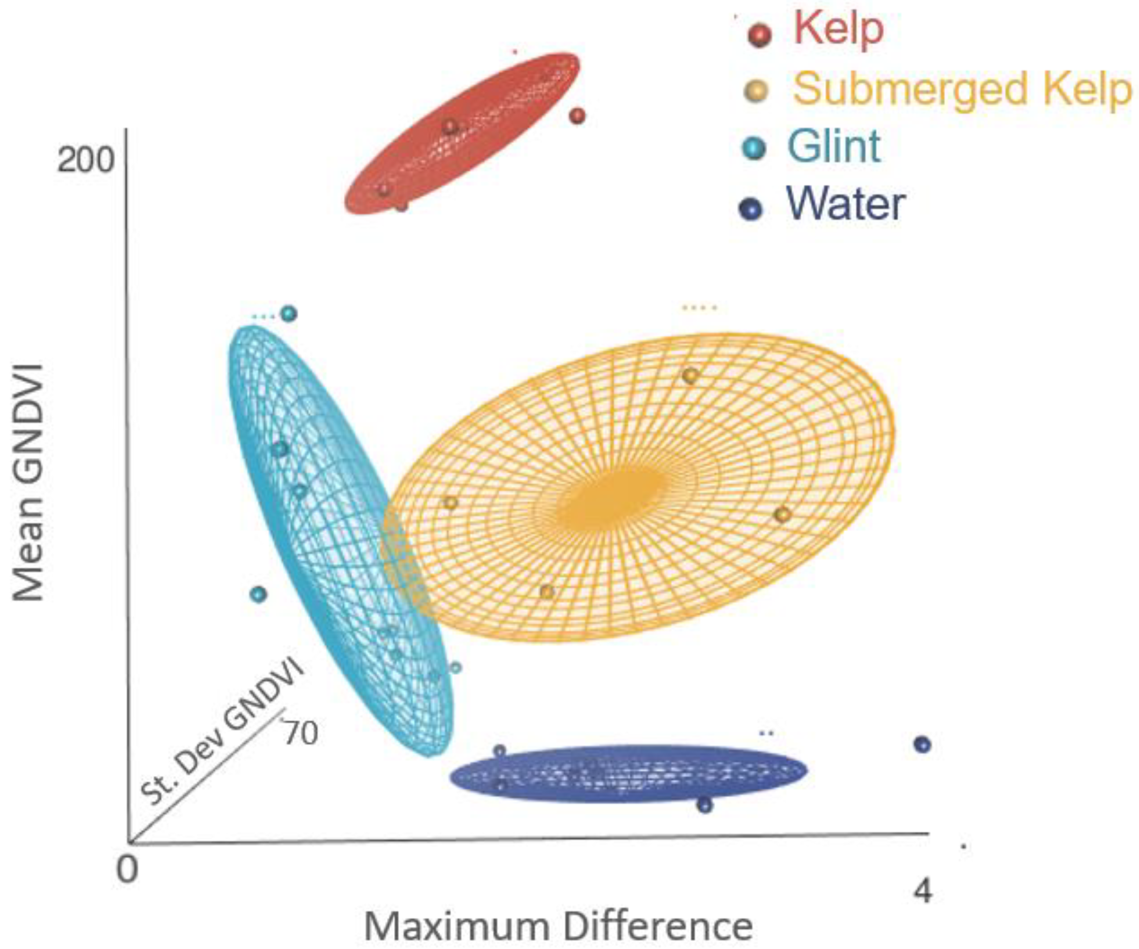
Band Indices/RatiosUse a measure of class separability such as the M-statistic to determine the best combination of band indices and ratios to use for each sensor. The most common band index used in floating kelp forest remote sensing is NDVI. However, we found G-NDVI, as well as band indices using the RedEdge band, often produced higher M-statistic scores.
ClassificationTo classify floating kelp area within different imagery from different satellites, use an adaptable OBIA classification with the help of the feature space optimization tool to minimize errors and attain high-accuracy scores. In this case, the feature space optimization tool often selected between three and 10 features depending on the image, with, generally, the mean of the red-edge band, the mean of the near-infrared band and/or the mean of the band indices selected. Of note, expert knowledge is required to choose samples to train the classifier and a visual quality assessment of the classification should be performed to minimize erroneous classifications prior to the accuracy assessment.
Accuracy AssessmentWhen possible, collect in situ validation data. However, if no ground-truth data are available, other forms of data can be used to validate the classification, such as past surveys that show the location of kelp forests, or expert knowledge based on reflectance values.
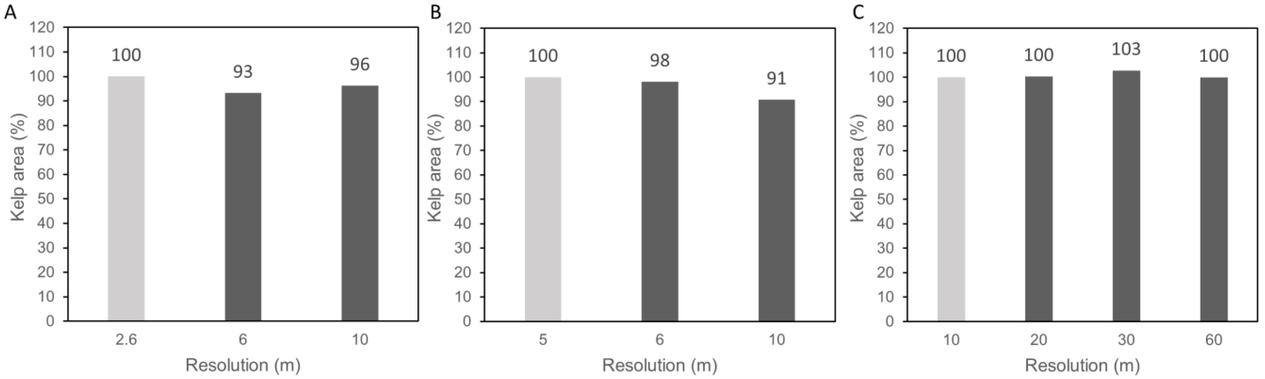
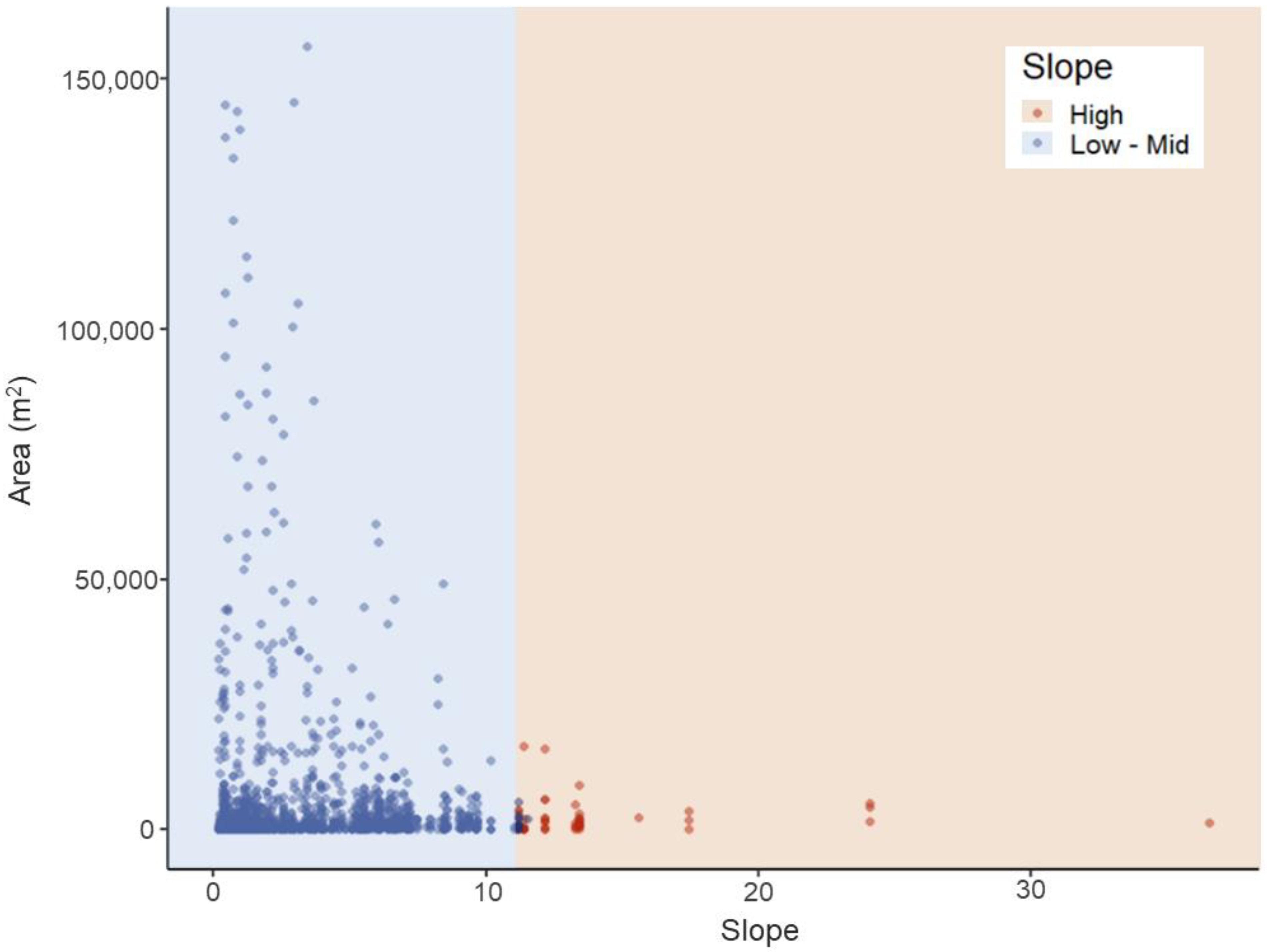
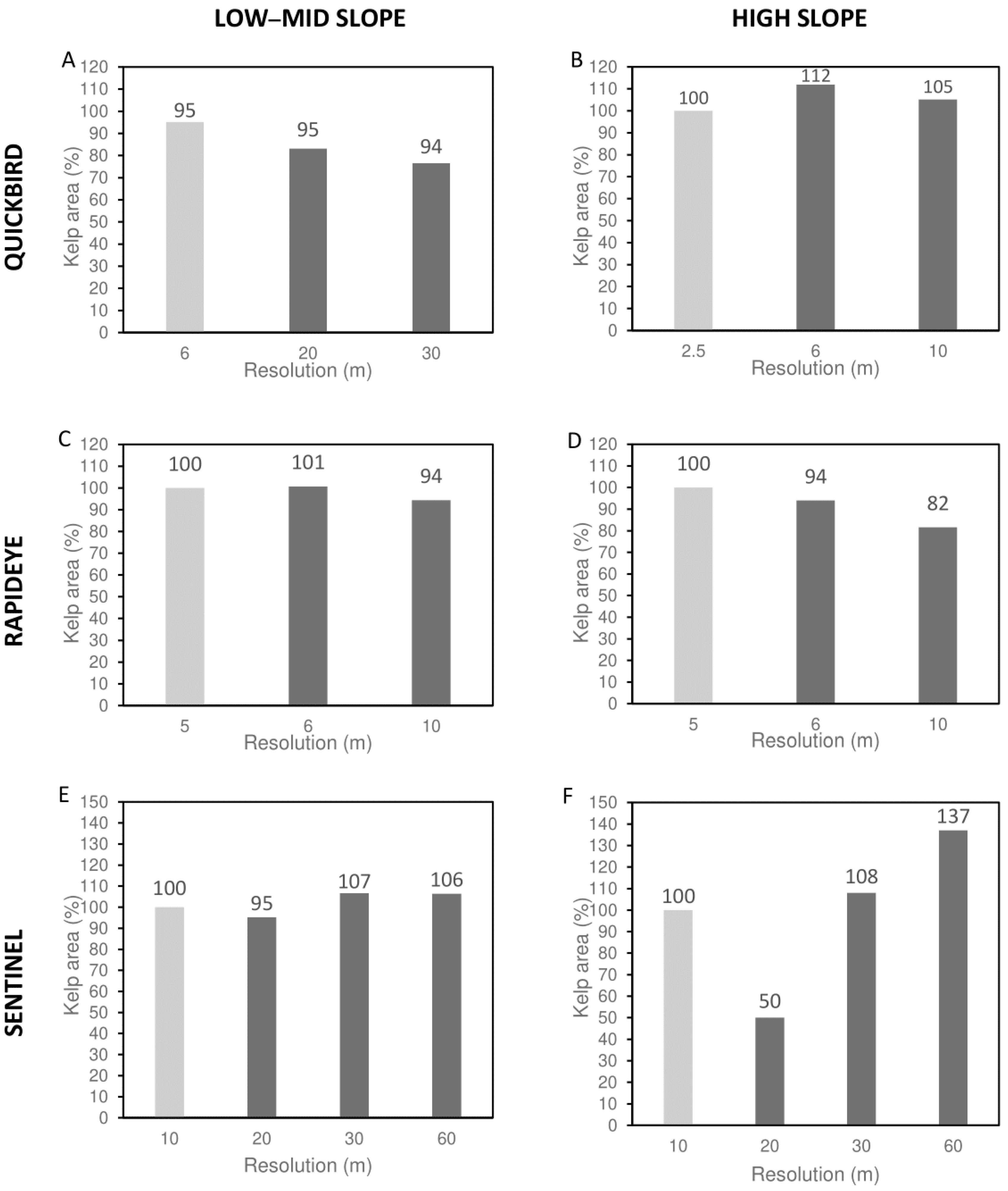
ResolutionThe ability to map floating kelp forests at different imagery resolutions can vary spatially based on ocean floor slope, and thus this metric can be used to highlight areas of uncertainty.
Based on the Haida Gwaii test area:
We suggest that regions with slopes higher than 11.4% should either be mapped only with the high-resolution imagery or excluded from comparisons between high- and medium-resolution imagery. We suggest that changes up to 7% be taken into consideration when comparing kelp distributions from imagery at different resolutions in low–mid slope areas.
Special attention should be given to the detection limits at different resolutions when applying the framework in new areas, thus we suggest performing similar resolution analyses and adjusting the ocean floor slope threshold accordingly, especially if segment size and kelp forest density and species vary significantly from those presented in this study.
Disclaimer/Publisher’s Note: The statements, opinions and data contained in all publications are solely those of the individual author(s) and contributor(s) and not of MDPI and/or the editor(s). MDPI and/or the editor(s) disclaim responsibility for any injury to people or property resulting from any ideas, methods, instructions or products referred to in the content.

