Arctic Sea Ice Concentration Assimilation in an Operational Global 1/10° Ocean Forecast System

Abstract

To understand the Arctic environment, which is closely related to sea ice and to reduce potential risks, reliable sea ice forecasts are indispensable. A practical, lightweight yet effective assimilation scheme of sea ice concentration based on Optimal Interpolation is designed and adopted in an operational global 1/10° surface wave-tide-circulation coupled ocean model (FIO-COM10) forecasting system to improve Arctic sea ice forecasting. Twin numerical experiments with and without data assimilation are designed for the simulation of the year 2019, and 5-day real-time forecasts for 2021 are implemented to study the sea ice forecast ability. The results show that the large biases in the simulation and forecast of sea ice concentration are remarkably reduced due to satellite observation uncertainty levels by data assimilation, indicating the high efficiency of the data assimilation scheme. The most significant improvement occurs in the marginal ice zones. The sea surface temperature bias averaged over the marginal ice zones is also reduced by 0.9 °C. Sea ice concentration assimilation has a profound effect on improving forecasting ability. The Root Mean Square Error and Integrated Ice-Edge Error are reduced to the level of the independent satellite observation at least for 24-h forecast, and sea ice forecast by FIO-COM10 has better performance than the persistence forecasts in summer and autumn.

1. Introduction

Arctic sea ice has experienced significant changes during the past few decades [1]. Arctic sea ice coverage has revealed a decreasing trend in the satellite era (1979-present) [2,3,4] and September Arctic sea ice extent is now shrinking by an average of 13.0% per decade according to National Snow and Ice Data Center (NSIDC) Sea Ice Index data (product identifier: G02135) [5].

This ongoing retreat of sea ice opens up new opportunities for more frequent human activities such as navigation through the Arctic Ocean [6,7]. Along with economic benefits, the decreasing Arctic sea ice can affect the oceanic environment through many aspects, e.g., changing circulation and overturning by affecting the salinity of the underlying ocean and leading to ecological consequences by threatening a wide range of Arctic wildlife [8,9]. Studies have shown that the changing of Arctic sea ice has a potential broad-range of climate consequences, such as increasing the extremes in the Arctic [4] and in the mid-latitudes of the Northern Hemisphere [10,11]. More reliable real-time simulations and forecasts of sea ice are in demand to reduce potential risks that threaten marine safety, and in turn, to benefit the ocean and climate simulations.

To understand the state and variations of the Arctic environment that are closely related to sea ice, and to provide sea ice forecasts and predictions, coupled sea ice-ocean models have been developed. There are many sea ice-ocean forecasting systems currently in use. Examples of sea ice-ocean forecasting systems that can provide Arctic sea ice prediction are the Global Ocean Forecast System (GOFS) 3.1 (GOFS 3.1) [12], the Canadian Global Ice Ocean Prediction System (GIOPS) [13], and the global Navy Earth System Prediction Capability (Navy-ESPC) [14]. The GOFS 3.1 provides short term, 1–7-day forecasts of global sea ice and ocean conditions with the sea ice model Community Ice CodE (CICE) two-way coupled to the HYbrid Coordinate Ocean Model (HYCOM). The GOFS 3.1 replaced the Arctic Cap Nowcast/Forecast System (ACNFS) for Arctic sea ice prediction, and the CICE model in the GOFS 3.1 is nearly the same as that employed by the ACNFS, which was validated by Hebert et al. [6]. The GIOPS provides daily global ice and ocean analyses with 10-day forecasts at the eddy-permitting resolution. The Navy ESPC V2 deterministic system is designed for operational forecasting for timescales of days (16-day forecast), and will replace GOFS 3.1 when it becomes operational (late 2023/early 2024). The global Navy ESPC V1 ensemble system became operational in 2021, providing 45-day forecasts on a weekly basis.

The sea ice predictive ability of a coupled ice–ocean model depends on the model itself and initialization. Data assimilation, though still a relatively new research area [15], has been demonstrated to be a useful technique to reduce the uncertainties in initialization and systematic errors in the model. However, the assimilation methods used can be quite different between these prediction systems. For example, an assimilation method varies according to the different initial model ice concentrations used in the ACNFS system [6], while a three-dimensional, multivariate (3DVAR) data assimilation scheme has been used in Navy-ESPC [14]. The Optimal Interpolation (OI) algorithm, as a feasible and effective method, has been applied in simulations and forecasts in many studies, such as by Zhang et al. [16], Stark et al. [17], and Wang et al. [18]. As a critical parameter of the polar marine environment, sea ice concentration is often taken as the primary observational parameter that is assimilated into forecasting systems to correct erroneous ice concentration estimates [9,19].

To meet operational demands, an operational global 1/10° surface wave-tide-circulation coupled ocean forecast system (FIO-COM10) has been developed and maintained by the First Institute of Oceanography, Ministry of Natural Resources, China [20]. The sea ice component is a critical component of FIO-COM10, especially for the polar region. Data assimilation of satellite-observed sea ice concentrations using an OI algorithm is employed in the global forecasting system FIO-COM10 to improve the sea ice forecasting ability. The main objective of this paper is to evaluate the performance of sea ice data assimilation and its impacts on the ocean simulations and forecasts up to 5 days by FIO-COM10. A detailed description of the model configuration, data assimilation scheme, and the observational data used is presented in Section 2. The results from the assimilation experiments and forecasting are given in Section 3. Discussion and conclusions are provided in Section 4.

2. Materials and Methods

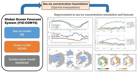
2.1. Model Description

The model employed in this study is the FIO-COM10 (

Table 1. Model configurations of FIO-COM10.

Model Components	Model Parameters/Schemes	Values/Configurations
Surface wave model MASNUM	Horizontal resolution	1/10° × 1/10°
	Spectral discretization	24 directions, 25 wave numbers
	Spatial coverage	global ocean
Ocean model MOM5	Horizontal resolution	1/10° × 1/10°
	Vertical levels	54 levels (min: 2 m)
	Spatial coverage	global ocean
	Horizontal grid	Tri-polar grid with bi-polar region set to north of 65°N
	Vertical grid	Z* coordinate configured with bottom partial cells
	Horizontal diffusivity	Bi-harmonic, diffusive velocities of 1.96 cm/s for momentum and 0.65 cm/s for tracers
	Vertical diffusivity	KPP + Bv
	Air-sea fluxes	NCEP/Bulk formula
	Model topography	ETOPO1
Sea ice model SIS	Ice thickness categories	5
	Ice bulk salinity	0.005 PSU
	Snow albedo	0.85
	Ice albedo	0.72
	Ice/ocean drag coefficient	$3.24\times {10}^{-4}$
	Ice surface roughness length	$5\times {10}^{-4} \mathrm{m}$

), which is from an operational global ocean forecast system with a horizontal resolution of 1/10° × 1/10°. Vertically, the model has 54 levels, and the vertical layer thickness increases from 2 m at the surface layer to about 366 m at the bottom layer. The FIO-COM10 consists of an ocean component model based on the Modular Ocean Model version 5 (MOM5) [21], a surface wave component model based on the third-generation MASNUM surface wave model [22], and a sea ice component model from the Sea Ice Simulator (SIS) [23]. The atmospheric forcing is from the global forecast system (GFS) operated by the National Centers for Environmental Prediction (NCEP), USA, including the surface air temperature, atmospheric pressure at the sea surface, wind at 10 m height, precipitation, specific humidity, and radiation fluxes. The air-sea fluxes are calculated by using the CORE bulk formula [24]. For the ocean component model of FIO-COM10, the most distinguishing feature is that the nonbreaking surface wave-induced vertical mixing (Bv) is incorporated into the K-profile parameterization (KPP) vertical mixing scheme in the ocean model [25,26,27]. The data assimilation scheme for ocean temperature and salinity is based on the Ensemble Adjustment Kalman Filter (EAKF) method [28]. For the seawater temperature and salinity, the observation data assimilated into FIO-COM10 includes the optimally interpolated microwave and infrared sea surface temperature (SST) observations (http://www.remss.com, last assess: 31 December 2021), maps of sea level anomalies (SLA) obtained from the Copernicus marine and environment monitoring service (CMEMS), and salinity and temperature profiles from Argo.

2.2. Sea Ice Data Assimilation Method

To assimilate the gridded sea ice concentration data, we use an OI algorithm in the sea-ice component of the coupled model. The analysis equations are given below:

$$x^a=x^b+K\left[y^0-H{x}^b\right]$$

(1)

$$K=P^b{H}^T{\left[{HP}^b{H}^T+R\right]}^{-1}$$

(2)

where $x$ denotes the state of sea ice concentration at all grid points ($m$). $x^a$ is the estimate of analysis state, $x^b$ is model background state, $y^o$ is observation, $H$ is an operator that interpolates model space into observation space, and $K$ is a gain matrix that is determined by the background error covariance matrix $P^b$ and the observation error covariance matrix $R$. Here, the observation errors are considered to be spatially uncorrelated, and thus $R$ is a diagonal matrix. Its diagonal elements are given with fixed observation error variance based on instrumental errors.

The background error covariance matrix $P^b$ is simply estimated by a parameterization, rather than by an ensemble method.

Given that sea ice concentration is only a single-level variable, the elements of $P^b$ that represent the covariance between two points of $\left(x_1,y_1\right)$ and $\left(x_2,y_2\right)$ in the two-dimensional space can be expressed as follows,

$$P^b\left(x_1,y_1,x_2,y_2\right)={\sigma }^{2}exp\left[-\frac{{\left(x_1-x_2\right)}^2}{L_x^2}-\frac{{\left(y_1-y_2\right)}^2}{L_y^2}\right]$$

(3)

where ${\sigma }^2$ is error variance, which is set to $2.5\times {10}^{-3}$, which is non-dimensional following sea ice concentration; $L_x$ and $L_y$ are the correlation lengths in zonal and meridional directions, respectively, and they are both set to five times the grid spacing in the module. The OI scheme adopts a 1-day window for assimilating the daily sea ice concentration data, which is consistent with the assimilated sea ice product (OSISAF). Thus, the diurnal variability of sea ice may be damped during the assimilation window period, while during the forecast period, the model is unconstrained. The scheme uses a localization strategy, in which the distance $d$ between the model point $\left(x_m,y_m\right)$ and the observation point $\left(x_0,y_0\right)$ is computed by the formula $d=\frac{{\left(x_0-x_m\right)}^2}{L_x^2}+\frac{{\left(y_0-y_m\right)}^2}{L_y^2}$, and the 10 nearest observations (an estimation of observations falling within the correlation length $L_x$ and $L_y$) surrounding the given model grid point are then chosen to affect the analysis field.

2.3. Data

2.3.1. Sea Ice Concentration

In this study, two daily sea ice concentration datasets are used. The ice concentration data used for the sea ice assimilation is the AMSR-2 sea ice concentration product of the EUMETSAT Ocean and Sea Ice Satellite Application Facility (OSISAF, www.osi-saf.org, last assess: 31 January 2022). This OSISAF data (product identifier: OSI-408) has a spatial resolution of about 10 km on the polar stereographic grid. It is applied using the hybrid algorithm and has been validated by comparing it with high-resolution manual ice charts [29].

For assimilation result assessment, a well-validated observational dataset that is independent from data used for assimilation is indispensable. The sea ice concentration data used for evaluation are from the National Snow and Ice Data Center (NSIDC) retrieved from the Special Sensor Microwave Imager/Sounder (SSMIS) passive microwave data (http://nsidc.org/data/docs/daac/nsidc0051_gsfc_seaice.gd.html, last access: 29 April 2022) [30]. This data has been mapped on a polar stereographic projection with a spatial resolution of 25 km. For derivation technique and algorithm, the revised NASA Team algorithm is applied together with a weather filter [31] to improve the ice mask. Note that the NSIDC ice concentration data are derived from different satellite sensors, and are processed by different algorithms from those of the OSISAF data, so it is independent of the OSISAF data used in the data assimilation. In this study, we assume the NSIDC data is the “truth” and evaluate the model performance against this dataset.

2.3.2. SST Dataset

SST data used for evaluation are the Global High Resolution SST Multi-Product Ensemble (GMPE), processed by the Met Office of the U.K. This near-real-time data is a Level-4 satellite-retrieved product on a regular 1/4°resolution global grid (obtained from http://marine.copernicus.eu/ with a product identifier SST_GLO_SST_L4_NRT_OBSERVATIONS_010_005, last access: 16 December 2020).

2.4. Numerical Experiments of Sea Ice Concentration Assimilation

To examine the impact of data assimilation of satellite-derived sea ice concentrations on sea ice and ocean simulations, twin numerical experiments, named NoSICasim and SICasim, are conducted, respectively. The two experiments are based on the FIO-COM10, and the original EAKF assimilation module for seawater temperature and salinity is disabled to focus on the impact of sea ice concentration assimilation.

The NoSICasim is a numerical experiment in which the sea ice concentration assimilation is turned off, while the experiment SICasim assimilates the OSISAF sea ice concentration. Therefore, using the experiment NoSICasim as the reference, the impact of assimilating sea ice concentration in the experiment SICasim can be evaluated and investigated.

Both numerical experiments of NoSICasim and SICasim cover the time period from 1 December 2018 to 31 July 2020. Snapshots from each daily run over the period 1 January 2019 to 31 December 2019 are used to evaluate the effects of sea ice concentration assimilation.

2.5. Real-Time Forecast of 2021

After examining the effect of sea ice concentration assimilation in the numerical experiments, sea ice concentration assimilation was enabled in the FIO-COM10 real-time operational forecasting system. The real-time forecasts of FIO-COM10 start at 12:00Z for each day, with the sea ice concentration assimilation applied at the same time as the forecasting system continues to yield a 5-day prediction. The forecasts from the period 1 January 2021 to 31 December 2021 were chosen to assess the forecasting ability for Arctic sea ice in this study.

For consistency, all model results and observations have been interpolated onto the polar stereographic projection of the NSIDC data, which is the main reference observation for assimilation assessing.

3. Results

Different satellite-derived sea ice concentration products have significant deviations due to different satellite sensors and algorithms. Even for certain data, such as the NSIDC data, estimates of the accuracy can vary depending on sea ice conditions, methods, and locations used in individual studies [32]. Sea ice concentration in regions of thin ice and regions with melt ponds present on the sea ice tends to be underestimated by passive microwave sensors such as AMSR2 [33]. The average accuracy of the algorithm that the NASA team used in the NSIDC data was reported to be within 5% in winter in a compact (high concentration) ice pack, while the accuracy could rise to 15% in the Arctic during summer when melt ponds are present on the sea ice. The average accuracy of the OSISAF data is 10% for the NH (Northern Hemisphere) product. There is more confidence in sea ice concentration data, with at least 15% ice concentration [19,34]. Therefore, we used a value of 15% representing observational error, and this value was taken as the threshold to calculate sea ice extent (cumulative areas of the grid cells with at least 15% ice concentration) and sea ice area (the integral sum of the product of sea ice concentration times the cell area for all cells with at least 15% ice concentration).

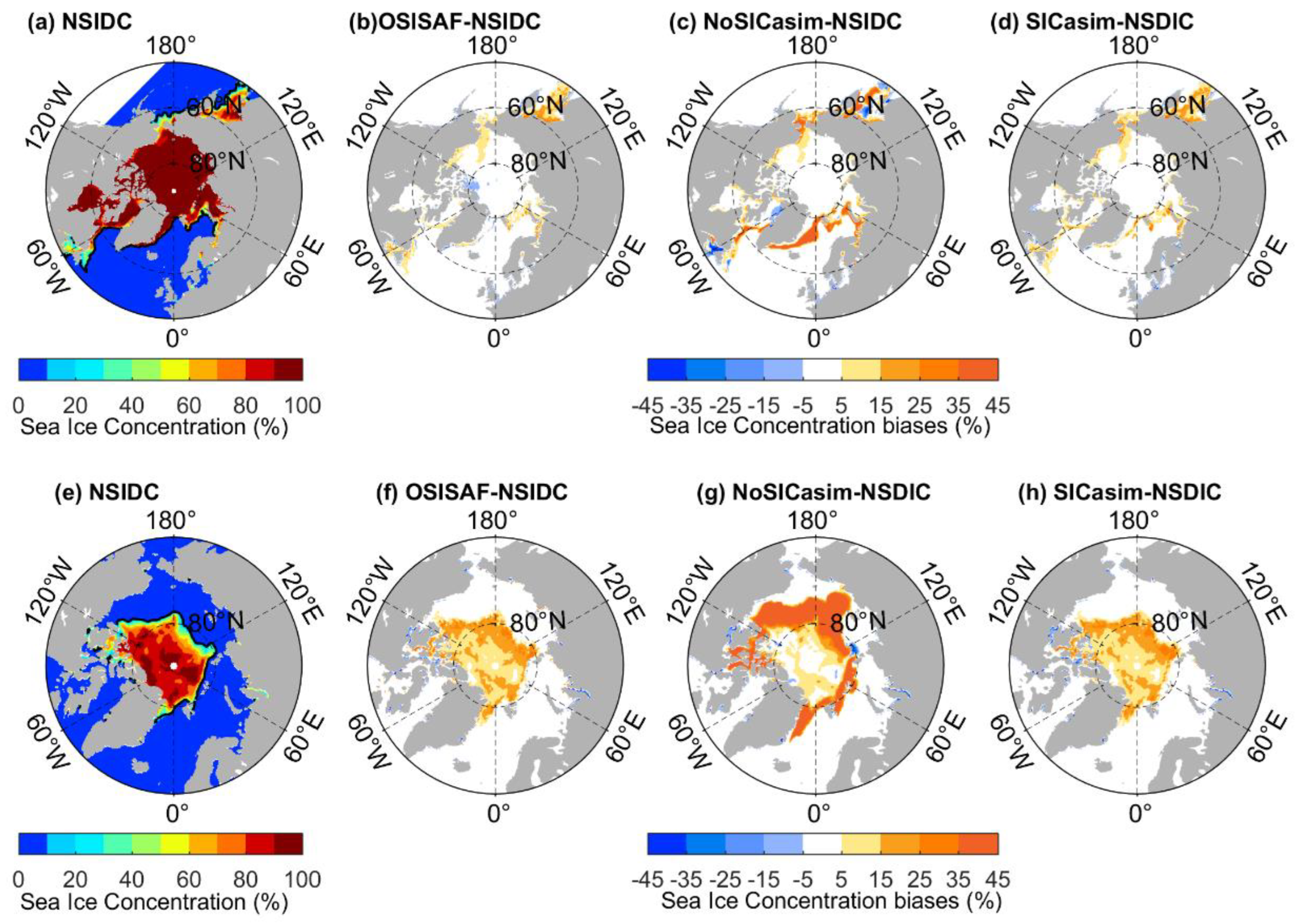
3.1. Performance of Sea Ice Assimilation

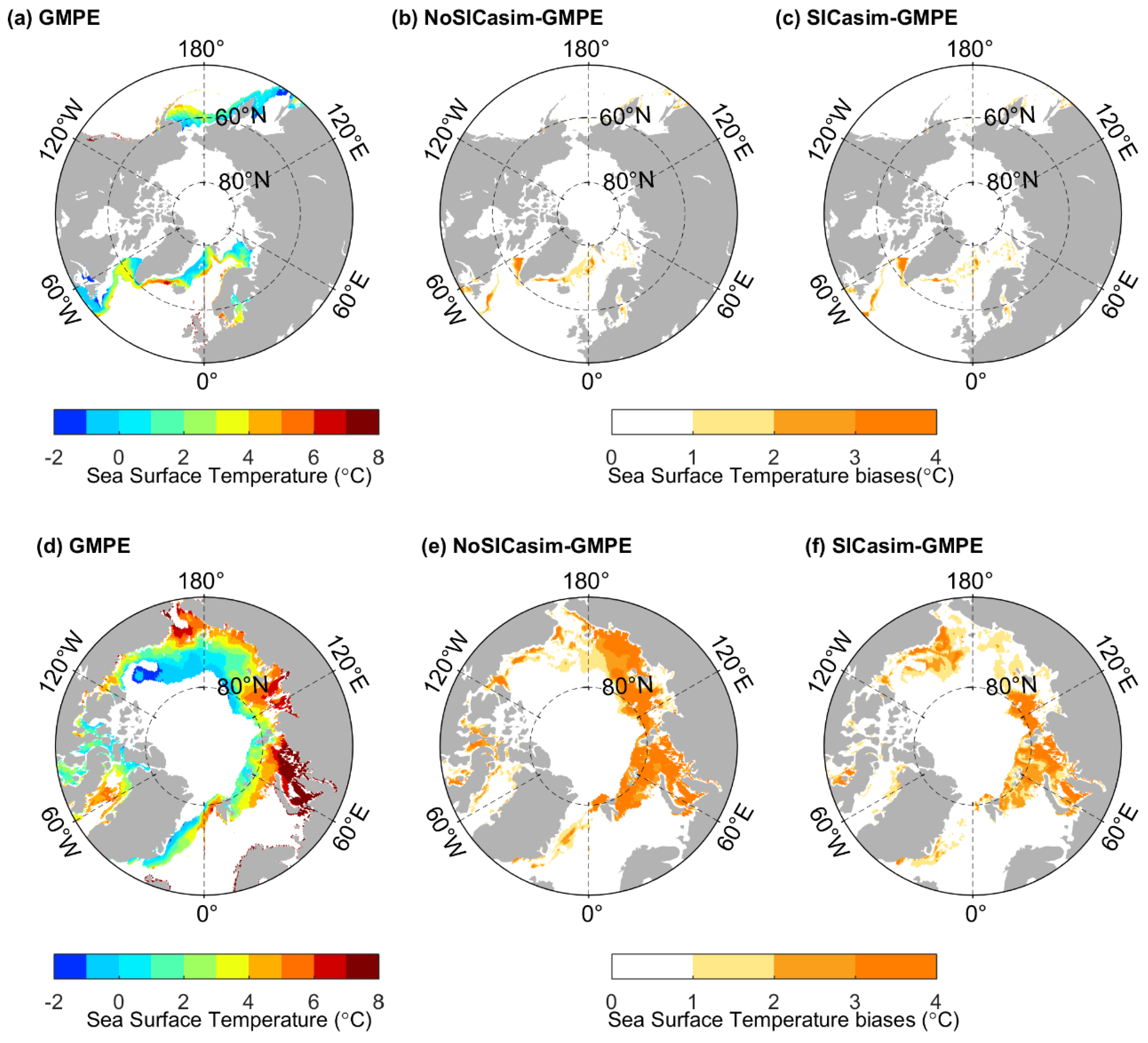
The sea ice concentration differences of simulations with and without data assimilation vary depending on the region and season. With the NSIDC sea ice concentration data regarded as the “truth”, we can take a glance at the impact of the assimilation simply by calculating the monthly averaged biases of the model simulations vs. the NSIDC observation (Figure 1). For reference, the biases between the OSISAF and NSIDC sea ice concentration data are also shown in Figure 1b, f. From the two observations, we can see that the most significant difference occurs in the marginal ice zone, while there is less difference in the compact ice pack (high concentration) areas. In winter, the sea ice concentration biases are much smaller than those in summer. The OSISAF sea ice concentration is slightly lower than the NSIDC observation in the high ice concentration area of Canadian Archipelago area and the Greenland Sea, while it is higher than the latter in the areas with low ice concentration, especially near the sea ice edge in the Chukchi, Bering, and Kara Seas and the Sea of Okhotsk. The corresponding Root Mean Square Error (RMSE) of regions with a sea ice concentration larger than 15% of the two datasets is lower in winter, with a value of 9–12% (figure not shown). However, in summer, it can reach up to 20%. This is mainly caused by the uncertainty due to increased variability in sea ice emissivity, the presence of melt ponds [35], and effects from oceanic processes, such as ocean surface waves and tides [7], etc. The ice concentration of OSISAF is generally higher than NSIDC in summer. Especially in the area near the sea ice edge; the deviation of the two can reach as high as 60%. Keeping these deviations in mind, the main metrics used to evaluate the assimilation performance are the bias, RMSE, and Integrated Ice-Edge Error (IIEE).

The effect of data assimilation can be seen by comparing the sea ice numerical experiments of NoSICasim and SICasim (Figure 1c vs. Figure 1d for March and Figure 1g vs. Figure 1h for September). The large error in experiment NoSICasim is remarkably reduced, especially in the low-concentration regions. In wintertime, not only is the strong overestimation of sea ice extent in the Greenland Sea corrected toward satellite observations, but also the overestimations of sea ice concentration, such as in the Labrador Sea, the Chukchi Sea, and the Sea of Okhotsk, as well as the underestimation in the Canadian Archipelago region, are improved in experiment SICasim. In summer, there is a large systematic bias of sea ice extent in experiment NoSICasim, which could be caused by errors in atmospheric forcing or uncertainties in model physics. This bias is corrected towards the true state by assimilating the observational sea ice concentration data. The erroneous patches of sea ice in the Canadian Archipelago region are also removed when assimilation is applied. Overall, the sea ice concentration is overestimated in the Arctic Ocean in experiment SICasim. However, note the deviations in sea ice concentration between the OSISAF and the NSIDC data; the biases in experiment SICasim are acceptable. The assimilation performance is closely related to the assimilation data used. We can assume that the model simulation can obtain a sea ice concentration dataset closer to the “truth” if the different observations have less difference and are closer to the real world.

The annual-mean RMSE (averaged from daily RMSE) of sea ice concentration with respect to the NSIDC data in Figure 2 shows that the biases are significantly reduced by the data assimilation. In experiment NoSICasim, RMSEs are larger than 20% in most regions of the Arctic Ocean (mainly the regions where sea ice in the satellite observation in summer does not exist), but the RMSEs are reduced to less than 10%, a level similar to the OSISAF data uncertainty. Eliminating the biases from the OSISAF data itself, the biases in experiment SICasim are mainly located in the marginal ice zones in summer when the minimum extent occurs, and in winter when the maximum extent occurs. This may be caused by the inappropriate SST simulation in areas with patches of sea ice, which is related to incoming atmospheric radiation, as suggested by Hebert et al. [6].

The temporal evolution of the mean RMSE of sea ice concentration with respect to the NSIDC data, which are regarded as the “truth” for 1 January to 31 December 2019, is shown in Figure 3. For the RMSE calculation, the criteria may vary in different studies. For example, areas where sea ice concentration is higher than 5%, either in the model or in observation, were chosen in Lisæter et al. [36], Strong [37], and Yang et al. [38]. With consideration to separating the performance in the compact ice areas and in the areas influenced by oceanic processes (such as ocean surface waves and tides), a sea ice concentration of 80% was additionally adopted as a criteria in Mu et al. [7]. Considering the accuracy of different observations mentioned above and following Mu et al. [7] to assess the data assimilation performance in the high-concentration areas, we calculated the averaged RMSE of areas with NSIDC observation between 15% and 80% (Figure 3a), and areas where the sea ice concentration of NSIDC observation is larger than 80% (Figure 3b), respectively.

The averaged RMSEs for the whole year of 2019 for numerical simulations of NoSICasim and SICasim, and the observational data OSISAF against the NSIDC data (as the “truth”) in the areas where the NSIDC concentration are larger than 15% and below 80%, are 34.5%, 22.4%, and 20.2%, respectively. The mean RMSE is greatly reduced by the assimilation scheme throughout the year (orange line vs. blue line). The RMSE of sea ice concentration in experiment SICasim shows varying biases for different seasons, with a bias trend similar to that of the OSISAF observation. The RMSE in experiment SICasim is slightly higher than that of the OSISAF observation before late March, but is then reduced and shows a quite similar level to the satellite observation errors from mid-April to late September. The RMSE of SICasim increases as new ice forms, but it is still much lower than the value of experiment NoSICasim. In the compact ice regions, the mean RMSE of experiment SICasim is comparable with that of the OSISAF concentration, except for the period from to 10 April to 30 July, and the RMSE in experiment SICasim during April to July leads to an annual mean RMSE of experiment SICasim (with a value of 6.9%) that is slightly higher than the OSISAF data (6.4%). Figure 3 shows that the impact of data assimilation is more pronounced in areas with relatively low sea ice concentrations.

The simulation of NoSICasim overestimates the sea ice area all through the year of 2019, and data assimilation results pull this value back to the observational uncertainty level. The sea ice area calculated from simulation SICasim is larger than that of the OSISAF data, but still lies within the deviation range between the two satellite observations used in this study (Figure 4a). In summer, the sea ice area of SICasim tends to have a similar value to that of OSISAF. Results of the sea ice extent are not shown, but they are similar to those of sea ice area.

The location of the sea ice edge is extremely important for marine safety [39]. The presence of the sea ice edge can lead to strong anisotropies and nonstationary features in the sea ice ocean system [36]. Therefore, the ice edge position is a critical variable of sea ice cover. We use the metric IIEE proposed by Goessling et al. [39] to assess data assimilation performance. Corresponding to the overestimation of sea ice extent (and thus, sea ice area), the simulation of NoSICasim has a large IIEE, especially in summer time (Figure 4b). The mean IIEE of experiment NoSICasim for the period from June to December is 1.93 × 10⁶ km², nearly 2.5 times larger than the value calculated from results of experiment SICasim, while this ratio decreases to 0.64 for the rest of 2019.

The performance of the sea ice edges simulation in experiment NoSICasim varies due to different regions and different seasons (Figure 5). For example, in March, other than a slight deviation from the NSIDC observation in the Bering Sea and the Sea of Okhotsk (Figure 5b), the main deviation occurs in the Greenland Sea (Figure 5c). The reason may be that this area is significantly affected by the convective process, and the model has some common problems in parameterization of this process [40,41]. Data assimilation of SICasim removes erroneous patches of sea ice in areas such as the Greenland Sea and the Bering Sea, and thus produces the sea ice edge much closer to the observation. In September (Figure 5d), as suggested by Liang et al. [42], the assimilation can have a better performance in terms of the sea ice edge simulation once SST is close to the freezing point, which, in our model, occurs in the areas between the sea ice edge of the NoSICasim experiment and that of the SICasim experiment. This improvement of IIEE may be attributed to a better representation of the surface energy balance in the marginal ice zones in the model simulations, as suggested by Lindsay and Zhang [19].

3.2. Impact on SST

The improvement of sea ice simulation has a profound impact on model simulation by effecting ocean state [17]; for example, effecting salt or heat fluxes. Since there are few observations for temperature and even less for salinity under sea ice in the central Arctic Ocean, we compare the simulated SST with GMPE SST and focus on the influence on SST by ice concentration assimilation in the areas with a sea ice concentration of less than 15% (Figure 6). According to Martin et al. [43], SST under the sea ice in GMPE is estimated using a variety schemes, and most of them are based on the estimation of freezing under sea ice. In our model, the SST under the sea ice is also the freezing of sea water. Therefore, the SST under the sea ice of GMPE and the model are comparable.

As the sea ice coverage biases are corrected through data assimilation of sea ice concentration, the experiment SICasim can provide a more reliable SST simulation in the area between the sea ice edge difference area of the NoSICasim and SICasim. SST simulations are greatly improved in the marginal ice zones, such as in the Greenland Sea in March and in the Canadian Archipelago, Greenland Sea, as well as Kara Sea regions in September. The mean SST uncertainties of the observational data are reported to be as high as 1.0 °C in most of the Arctic marginal seas [42]. The large averaged SST biases of about 1.1 °C between the results of experiment NoSICasim and the observations are reduced to 0.22 °C by data assimilation. This improvement in SST has potential influence on ocean state simulation, such as improving surface flux estimates [44] and convection simulation in the Greenland Sea.

In winter time, there is a systematic SST bias in the Labrador Sea for the NoSICasim, which is not corrected by data assimilation. This usually happens when the systematic SST bias is too large, as pointed out by Liang et al. [42]. In summer time, the SST bias in the Barents Sea and Kara Sea, which cannot be reduced by the present sea ice concentration data assimilation, may need additional SST data assimilation.

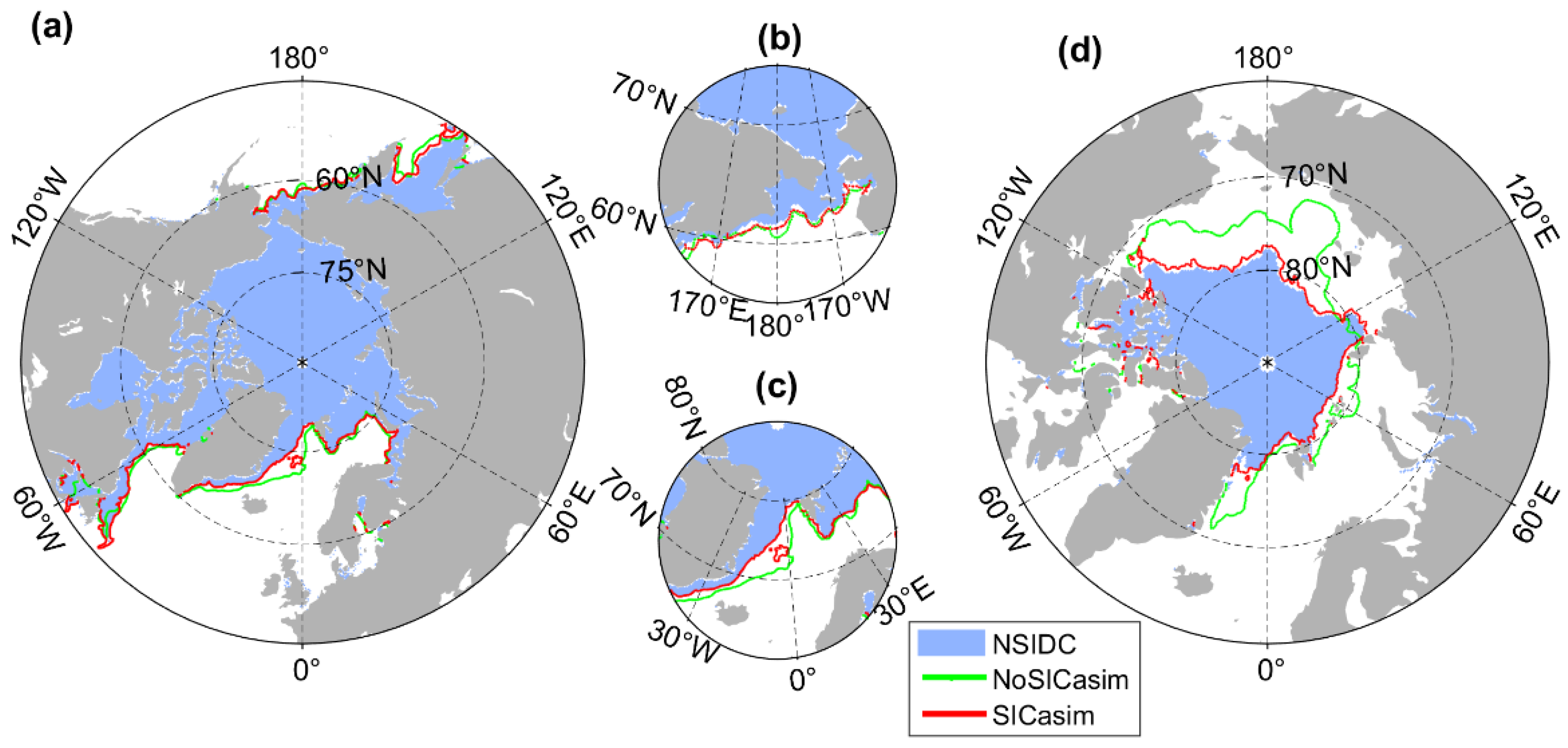
3.3. Impacts on Real-Time Sea Ice Forecasts

Motivated by the results of data assimilation numerical experiments, the data assimilation of sea ice concentration is implemented into the operational global 1/10° surface wave-tide-circulation coupled ocean forecast system (FIO-COM10) to improve its sea ice forecast ability. Since there are differences between different sea ice concentration datasets themselves, we chose the assimilated OSISAF data as the “truth” when evaluating forecasts, just as Stark et al. [17] did. A reforecast without sea ice concentration assimilation from the model period from 1 August to 30 September 2021 is implemented. After ~25 days, the forecasts without sea ice concentration assimilation become stable. We can clearly see the improvement of forecast ability by applying sea ice concentration assimilation from the comparison between the forecasts with and without sea ice concentration assimilation, both for RMSE and IIEE (Figure 7).

Spatially, the forecast performance varies in different regions, which is quite similar to that of the SICasim numerical experiment. There are relatively large concentration biases in forecasts in the marginal areas, such as the Canadian Archipelago, Greenland, and Okhotsk regions (figure not shown). Here, we present the forecast performance in sea ice concentration RMSE averaged for each month over the Arctic domain, a region with existing summer sea ice and with more frequent human activities (Figure 8a). The monthly averaged sea ice concentration RMSE eliminates the high frequency variations in daily resolution (figure not shown), but the overall trends of the two are highly consistent. As expected, the sea ice concentration RMSEs increase from 24 to 120 h (Figure 8b). For the sea ice concentration RMSE, a 24-h forecast is slightly higher than that of NSIDC data in spring and winter times, but is lower than the latter in the period from sea ice melting to new ice formatting. The overall performance of 24-h forecasting is at a similar level as the independent NSIDC data.

For annual-mean concentration RMSE, the forecasting system has a value slightly higher than persistence forecasts, i.e., an unchanging forecast for 24, 48 and 72 h, but has a superior performance than the latter for 96 and 120 h (Figure 8c). When the period is limited between August and November, a period with more human activities such as scientific investigation and commercial activities in the Arctic Ocean, the forecasting system has a better performance than persistence forecasts from 48 h (Figure 8d). The sea ice concentration forecasts can be taken as a reference for shipping routes with a 2–5 days lead-time.

The forecast results for IIEE are shown in Figure 9. Similar to that of RMSE, forecast performances degrade from 24 to 120 h, and forecasts on all time scales share similar trends. The IIEE of the 24-h forecast is lower than that of the NSIDC data for all months, meaning it lies within the satellite observation uncertainty range. In late spring and summer time, even the 72-h forecast has a reliable performance in the IIEE estimation.

The annual-mean IIEE of the forecasts is slightly higher than persistence forecasts, which could be attributed to errors in atmospheric forcing or uncertainties in model physics. However, the forecasting system can produce reliable sea ice edge predictions, and has outstanding performance for 48 to 120 h between August and November for the Northern Hemisphere (Figure 9c).

The choice of “reference” will influence the statistics of evaluation of forecast. When taking the NSIDC as reference, the RMSE and IIEE time series for 2021 for each forecast time are at the same level as those of OSISAF. The forecast has a slightly worse performance than the persistence forecast for RMSE, while it is better than the latter for IIEE (figure not shown). The statistics of the evaluation are closely related to the assimilation data used. We assume the forecasts will have a consistent performance if the different observations have less difference.

4. Discussion

Data assimilation is thought to be a useful technique to reduce the uncertainties in initialization and systematic errors in the numerical model. For better understanding of sea ice concentration assimilation performance, we compared the results of model simulation with and without assimilation. Overall, the large biases in ice concentration simulation could be significantly reduced by sea ice concentration assimilation, not only for the sea ice edge estimation, but also for the value of the ice concentration itself. The performance of concentration assimilation varied according to different regions and seasons, and the most significant improvement occurred in the marginal ice zones. For several scattered areas, the large biases in annual-mean RMSE of sea ice concentration in marginal ice zones that could not be corrected by this OI data assimilation may be related to inappropriate SST simulation, which could be related to inappropriate incoming atmospheric radiation, as suggested by Hebert et al. [6].

In addition to the direct effects on the sea ice itself, the improvement in sea ice simulation could have profound indirect effects on the simulation of other ocean variables; for example, salt content [19], ocean circulation [8], SST [42], and thus the sea ice state in the subsequent seasons [45]. In our study, the significant improvement in SST simulation was made more robust by the sea ice concentration data assimilation, and these improvements were mainly achieved through improvements in sea ice coverage simulation. There were still some systematic SST biases that could not be corrected by sea ice concentration assimilation in the marginal areas, such as the Labrador Sea. This may need implementing an additional SST assimilation and considering the covariance between SST and sea ice concentration [36,46].

5. Conclusions

For a real-time operational forecast system, an effective and low-cost data assimilation scheme is desirable. In this study, a practical, lightweight yet effective data assimilation scheme of sea ice concentration based on the OI algorithm was designed and used to assimilate satellite-derived sea-ice concentration data into an operational global ocean forecast system. The data assimilation performance and assimilation effect in forecasting system were investigated and evaluated using results from twin numerical experiments with and without data assimilation in 2019, and from 5 days operational forecasting evaluation in 2021, respectively. To assess the assimilation performance in different concentration areas, the averaged RMSE with respect to the NSIDC observation in the areas with sea ice concentration of the NSIDC data between 15% and 80%, and in the areas where the NSIDC observation are larger than 80%, were calculated, respectively. The results showed that the effect of concentration assimilation was more pronounced in areas with relatively low sea ice concentrations, where sea ice is supposed to be significantly influenced by oceanic processes, such as ocean surface waves and tides. To assess the assimilation effect on the operational ocean forecasting system, we focused on two metrics: RMSE and IIEE. The relatively large concentration biases in forecasts in the marginal areas, such as the Sea of Okhotsk, were not surprising due to the original deviation between the observations. Both sea ice concentration RMSEs and IIEEs increased from 24 to 120 h. For RMSEs, the best performances were derived from 24-h forecasting, with a similar level as the independent NSIDC data. For IIEEs, even the 72-h forecast had a reliable performance and was within the satellite observation uncertainty range. From August to November, a period with more human activity in the Arctic Ocean, the forecasting system had a much better performance than the persistence forecast; i.e., an unchanging forecast with a 2–5 days lead-time for sea ice concentration and sea ice edge location.

In summary, by applying a practical, lightweight yet effective sea ice concentration assimilation scheme, the simulated and forecast sea ice concentration and edges of Arctic in our operational global ocean-ice coupled forecast system were significantly improved. Furthermore, the simulated SST of the Arctic was also improved due to sea ice concentration assimilation. Since the ocean-ice model adopted in this study (MOM5 and SIS) is widely used in the ocean climate modeling community, we believe that the practical scheme can shed light on other ocean climate numerical experiments to improve the simulation of polar region.

The model errors could be ascribed to varying aspects of spatial errors (e.g., a shift in the location of a formation event) to the misrepresentation of physical processes [13,14,38]. There is no doubt that the model’s forecast ability can be improved by including more reasonable physical processes and by employing more realistic parameterizations. We showed in this study the impact of sea ice concentration data assimilation in the coupled ocean model FIO-COM10 on sea ice concentration forecast. There is still potential for further optimization; for example, by employing SST and sea ice thickness data assimilation, upgrading the convection scheme in the Greenland Sea, and increasing vertical and horizontal resolutions. These will be explored in future studies.

References

1. Cavalieri, D.J.; Parkinson, C.L. Arctic sea ice variability and trends, 1979–2010. Cryosphere 2012, 6, 881–889. [Google Scholar] [CrossRef] [Green Version]
2. Comiso, J.C.; Parkinson, C.L.; Gersten, R.; Stock, L. Accelerated decline in the Arctic sea ice cover. Geophys. Res. Lett. 2008, 35, L01703. [Google Scholar] [CrossRef] [Green Version]
3. Gao, Y.; Sun, J.; Li, F.; He, S.; Sandven, S.; Yan, Q.; Zhang, Z.; Lohmann, K.; Keenlyside, N.; Furevik, T.; et al. Arctic sea ice and Eurasian climate: A review. Adv. Atmos. Sci. 2015, 32, 92–114. [Google Scholar] [CrossRef] [Green Version]
4. Landrum, L.; Holland, M.M. Extremes become routine in an emerging new Arctic. Nat. Clim. Chang. 2020, 10, 1108–1115. [Google Scholar] [CrossRef]
5. Meier, W.N.; Perovich, D.; Farrell, S.; Haas, C.; Hendricks, S.; Petty, A.A.; Webster, M.; Divine, D.; Gerland, S.; Kaleschke, L.; et al. Sea Ice. NOAA Technical Report OAR ARC. 2021. Available online: https://repository.library.noaa.gov/view/noaa/34474 (accessed on 7 February 2023).
6. Hebert, D.A.; Allard, R.A.; Metzger, E.J.; Posey, P.G.; Preller, R.H.; Wallcraft, A.J.; Phelps, M.W.; Smedstad, O.M. Short-term sea ice forecasting: An assessment of ice concentration and ice drift forecasts using the U.S. Navy’s Arctic Cap Nowcast/Forecast System. J. Geophys. Res. Ocean. 2015, 120, 8327–8345. [Google Scholar] [CrossRef] [Green Version]
7. Mu, L.; Liang, X.; Yang, Q.; Liu, J.; Zheng, F. Arctic Ice Ocean Prediction System: Evaluating sea-ice forecasts during Xuelong’s first trans-Arctic Passage in summer 2017. J. Glaciol. 2019, 65, 813–821. [Google Scholar] [CrossRef] [Green Version]
8. Parkinson, C.L.; Cavalieri, D.J. Arctic sea ice variability and trends, 1979–2006. J. Geophys. Res. Ocean. 2008, 113, C07003. [Google Scholar] [CrossRef] [Green Version]
9. Shu, Q.; Qiao, F.; Liu, J.; Song, Z.; Chen, Z.; Zhao, J.; Yin, X.; Song, Y. Arctic sea ice concentration and thickness data assimilation in the FIO-ESM climate forecast system. Acta Oceanol. Sin. 2021, 40, 65–75. [Google Scholar] [CrossRef]
10. Liu, J.; Curry, J.A.; Wang, H.; Song, M.; Horton, R.M. Impact of declining Arctic sea ice on winter snowfall. Proc. Natl. Acad. Sci. USA 2012, 109, 4074–4079. [Google Scholar] [CrossRef] [Green Version]
11. Mori, M.; Watanabe, M.; Shiogama, H.; Inoue, J.; Kimoto, M. Robust Arctic sea-ice influence on the frequent Eurasian cold winters in past decades. Nat. Geosci. 2014, 7, 869–873. [Google Scholar] [CrossRef]
12. Metzger, E.J.; Helber, R.W.; Hogan, P.J.; Posey, P.G.; Thoppil, P.G.; Townsend, T.L.; Wallcraft, A.J.; Smedstad, O.M.; Franklin, D.S.; Zamudo-Lopez, L.; et al. Global Ocean Forecast System 3.1 Validation Test; NRL/MR/7320–17-9722; Stennis Space Center: Hancock, MS, USA, 2017. [Google Scholar]
13. Smith, G.C.; Roy, F.; Reszka, M.; Surcel Colan, D.; He, Z.; Deacu, D.; Belanger, J.-M.; Skachko, S.; Liu, Y.; Dupont, F.; et al. Sea ice forecast verification in the Canadian Global Ice Ocean Prediction System. Q. J. R. Meteorol. Soc. 2016, 142, 659–671. [Google Scholar] [CrossRef] [Green Version]
14. Barton, N.; Metzger, E.J.; Reynolds, C.A.; Ruston, B.; Rowley, C.; Smedstad, O.M.; Ridout, J.A.; Wallcraft, A.; Frolov, S.; Hogan, P.; et al. The Navy’s Earth System Prediction Capability: A New Global Coupled Atmosphere-Ocean-Sea Ice Prediction System Designed for Daily to Subseasonal Forecasting. Earth Space Sci. 2021, 8, e2020EA001199. [Google Scholar] [CrossRef]
15. Liu, J.; Chen, Z.; Hu, Y.; Zhang, Y.; Ding, Y.; Cheng, X.; Yang, Q.; Nerger, L.; Spreen, G.; Horton, R.; et al. Towards reliable Arctic sea ice prediction using multivariate data assimilation. Sci. Bull. 2019, 64, 63–72. [Google Scholar] [CrossRef] [PubMed] [Green Version]
16. Zhang, J.; Thomas, D.R.; Rothrock, D.A.; Lindsay, R.W.; Yu, Y.; Kwok, R. Assimilation of ice motion observations and comparisons with submarine ice thickness data. J. Geophys. Res. Ocean. 2003, 108, 3170. [Google Scholar] [CrossRef] [Green Version]
17. Stark, J.D.; Ridley, J.; Martin, M.; Hines, A. Sea ice concentration and motion assimilation in a sea ice−ocean model. J. Geophys. Res. Ocean. 2008, 113, C05S91. [Google Scholar] [CrossRef]
18. Wang, K.; Debernard, J.B.; Sperrevik, A.K.; Isachsen, P.E.; Lavergne, T. A combined optimal interpolation and nudging scheme to assimilate OSISAF sea-ice concentration into ROMS. Ann. Glaciol. 2013, 54, 8–12. [Google Scholar] [CrossRef] [Green Version]
19. Lindsay, R.W.; Zhang, J. Assimilation of Ice Concentration in an Ice–Ocean Model. J. Atmos. Ocean. Technol. 2006, 23, 742–749. [Google Scholar] [CrossRef] [Green Version]
20. Sun, Y.; Perrie, W.; Qiao, F.; Wang, G. Intercomparisons of High-Resolution Global Ocean Analyses: Evaluation of A New Synthesis in Tropical Oceans. J. Geophys. Res. Ocean. 2020, 125, e2020JC016118. [Google Scholar] [CrossRef]
21. Griffies, S.M. Elements of the Modular Ocean Model (MOM) (2012 Release with Updates); NOAA/Geophysical Fluid Dynamics Laboratory: Princeton, NJ, USA, 2012; pp. 614–627. [Google Scholar]
22. Qiao, F.; Zhao, W.; Yin, X.; Huang, X.; Liu, X.; Shu, Q.; Wang, G.; Song, Z.; Li, X.; Liu, H.; et al. A Highly Effective Global Surface Wave Numerical Simulation with Ultra-High Resolution. In Proceedings of the SC16: International Conference for High Performance Computing, Networking, Storage and Analysis, Salt Lake City, UT, USA, 13–18 November 2016; pp. 46–56. [Google Scholar]
23. Winton, M. A Reformulated Three-Layer Sea Ice Model. J. Atmos. Ocean. Technol. 2000, 17, 525–531. [Google Scholar] [CrossRef]
24. Large, G.; Yeager, S.G. Diurnal to Decadal Global Forcing for Ocean and Sea-Ice Models: The Data Sets and Flux Climatologies (No. NCAR/TN-460+STR); University Corporation for Atmospheric Research: Boulder, CO, USA, 2004; Available online: https://opensky.ucar.edu/islandora/object/technotes:434 (accessed on 1 February 2023).
25. Qiao, F.; Yang, Y.; Xia, C.; Yuan, Y. The role of surface waves in the ocean mixed layer. Acta Oceanol. Sin. 2008, 27, 30–37. [Google Scholar]
26. Qiao, F.; Yuan, Y.; Deng, J.; Dai, D.; Song, Z. Wave–turbulence interaction-induced vertical mixing and its effects in ocean and climate models. Philos. Trans. R. Soc. A Math. Phys. Eng. Sci. 2016, 374, 20150201. [Google Scholar] [CrossRef] [Green Version]
27. Qiao, F.; Yuan, Y.; Yang, Y.; Zheng, Q.; Xia, C.; Ma, J. Wave-induced mixing in the upper ocean: Distribution and application to a global ocean circulation model. Geophys. Res. Lett. 2004, 31, L11303. [Google Scholar] [CrossRef]
28. Yin, X.; Qiao, F.; Shu, Q. Using ensemble adjustment Kalman filter to assimilate Argo profiles in a global OGCM. Ocean Dyn. 2011, 61, 1017–1031. [Google Scholar] [CrossRef] [Green Version]
29. Lavelle, J.; Tonboe, R.; Tian, T.; Pfeiffer, R.-H.; Howe, E. Product User Manual for the OSI SAF AMSR-2 Global Sea Ice Concentration; Product OSI-408; Danish Meteorological Institute: Copenhagen, Denmark, 2016. [Google Scholar]
30. Cavalieri, D.J.; Parkinson, C.L.; Gloersen, P.; Zwally, H.J.; DiGirolamo, N. Sea Ice Concentrations from Nimbus-7 SMMR and DMSP SSM/I-SSMIS Passive Microwave Data; Version 2 [NSIDC-0051]; NASA National Snow and Ice Data Center Distributed Active Archive Center: Boulder, CO, USA, 2022. [Google Scholar] [CrossRef]
31. Cavalieri, D.J.; Germain, K.M.S.; Swift, C.T. Reduction of weather effects in the calculation of sea-ice concentration with the DMSP SSM/I. J. Glaciol. 1995, 41, 455–464. [Google Scholar] [CrossRef] [Green Version]
32. Cavalieri, D.J.; Crawford, J.; Drinkwater, M.; Emery, W.J.; Eppler, D.T.; Farmer, L.D.; Goodberlet, M.; Jentz, R.; Milman, A.; Morris, C.; et al. NASA Sea Ice Validation Program for the DMSP SSM/I: Final Report; National Aeronautics and Space Administration: Washington, DC, USA, 1992. [Google Scholar]
33. Meier, W.N.; Fetterer, F.; Stewart, J.S.; Helfrich, S. How do sea-ice concentrations from operational data compare with passive microwave estimates? Implications for improved model evaluations and forecasting. Ann. Glaciol. 2015, 56, 332–340. [Google Scholar] [CrossRef] [Green Version]
34. Tonboe, R.; Nielsen, E. Global Sea Ice Concentration Reprocessing Validation Report; European Organisation for the Exploitation of Meteorological Satellites (EUMETSAT) Ocean and Sea Ice Satellite Application Facility: Darmstadt/Boulder, CO, USA, 2010. [Google Scholar]
35. Ivanova, N.; Pedersen, L.T.; Tonboe, R.T.; Kern, S.; Heygster, G.; Lavergne, T.; Sørensen, A.; Saldo, R.; Dybkjær, G.; Brucker, L.; et al. Inter-comparison and evaluation of sea ice algorithms: Towards further identification of challenges and optimal approach using passive microwave observations. Cryosphere 2015, 9, 1797–1817. [Google Scholar] [CrossRef] [Green Version]
36. Lisæter, K.A.; Rosanova, J.; Evensen, G. Assimilation of ice concentration in a coupled ice–ocean model, using the Ensemble Kalman filter. Ocean Dyn. 2003, 53, 368–388. [Google Scholar] [CrossRef]
37. Strong, C. Atmospheric influence on Arctic marginal ice zone position and width in the Atlantic sector, February–April 1979–2010. Clim. Dyn. 2012, 39, 3091–3102. [Google Scholar] [CrossRef]
38. Yang, Q.; Losa, S.N.; Losch, M.; Liu, J.; Zhang, Z.; Nerger, L.; Yang, H. Assimilating summer sea-ice concentration into a coupled ice–ocean model using a LSEIK filter. Ann. Glaciol. 2015, 56, 38–44. [Google Scholar] [CrossRef] [Green Version]
39. Goessling, H.F.; Tietsche, S.; Day, J.J.; Hawkins, E.; Jung, T. Predictability of the Arctic sea ice edge. Geophys. Res. Lett. 2016, 43, 1642–1650. [Google Scholar] [CrossRef] [Green Version]
40. Mikolajewicz, U.; Sein, D.V.; Jacob, D.; Königk, T.; Podzun, R.; Semmler, T. Simulating Arctic sea ice variability with a coupled regional atmosphere-ocean-sea ice model. Meteorol. Z. 2005, 14, 793–800. [Google Scholar] [CrossRef] [Green Version]
41. Wadhams, P. Arctic sea ice extent and thickness. In The Arctic and Environmental Change; Dowdeswell, J.A., Ed.; Routledge: London, UK, 2019; pp. 101–119. [Google Scholar] [CrossRef]
42. Liang, X.; Losch, M.; Nerger, L.; Mu, L.; Yang, Q.; Liu, C. Using Sea Surface Temperature Observations to Constrain Upper Ocean Properties in an Arctic Sea Ice-Ocean Data Assimilation System. J. Geophys. Res. Ocean. 2019, 124, 4727–4743. [Google Scholar] [CrossRef]
43. Martin, M.; Dash, P.; Ignatov, A.; Banzon, V.; Beggs, H.; Brasnett, B.; Cayula, J.-F.; Cummings, J.; Donlon, C.; Gentemann, C.; et al. Group for High Resolution Sea Surface temperature (GHRSST) analysis fields inter-comparisons. Part 1: A GHRSST multi-product ensemble (GMPE). Deep Sea Res. Part II Top. Stud. Oceanogr. 2012, 77–80, 21–30. [Google Scholar] [CrossRef]
44. While, J.; Martin, M.J. Variational bias correction of satellite sea-surface temperature data incorporating observations of the bias. Q. J. R. Meteorol. Soc. 2019, 145, 2733–2754. [Google Scholar] [CrossRef]
45. Blanchard-Wrigglesworth, E.; Armour, K.C.; Bitz, C.M.; DeWeaver, E. Persistence and Inherent Predictability of Arctic Sea Ice in a GCM Ensemble and Observations. J. Clim. 2011, 24, 231–250. [Google Scholar] [CrossRef]
46. Frolov, S.; Bishop, C.H.; Holt, T.; Cummings, J.; Kuhl, D. Facilitating Strongly Coupled Ocean–Atmosphere Data Assimilation with an Interface Solver. Mon. Weather Rev. 2016, 144, 3–20. [Google Scholar] [CrossRef]
Figure 1. Arctic sea ice concentration from NSIDC (a,e) which is regarded as the “truth”, the biases of OSISAF (b,f) and model biases (c,d,g,h) of the Northern Hemisphere in March (ad) and September (eh), 2019.
Remotesensing 15 01274 g001
Figure 2. Annual-mean RMSE of Arctic sea ice concentration of the OSISAF observation (a), the numerical experiment NoSICasim (b), and the numerical experiment SICasim (c) with respect to the NSIDC observation during 2019.
Remotesensing 15 01274 g002
Figure 3. The RMSE time series of sea ice concentration with respect to the NSIDC observation of the Northern Hemisphere from 1 January to 31 December 2019. The results of experiments NoSICasim and SICasim are shown in blue and orange, respectively. The RMSE time series of OSISAF with respect to the NSIDC observation is shown in gray. Note that (a) is computed over the area where the NSIDC observation is larger than 15% and below 80%, and (b) is computed over the area where the NSIDC observation is larger than 80%. Date format for x-axis is day/month.
Remotesensing 15 01274 g003
Figure 4. Sea ice area (a) and IIEE (b) time series in the Arctic region from 1 January to 31 December 2019. The experiments without and with data assimilation are shown in blue and orange, respectively. Sea ice areas of NSIDC and OSISAF are shown in green and gray, respectively. IIEEs between NSIDC and OSISAF are shown in gray.
Remotesensing 15 01274 g004
Figure 5. Simulated and observed sea ice edge locations in March (ac) and September 2019 (d). Areas where sea ice concentration in the NSIDC observation is higher than 15% are denoted by the blue patch. The ice edges in the experiments NoSICasim and SICasim are denoted by green and red lines, respectively. Note that (b,c) show the same data as (a), but are zoomed in on the Bering Sea and the Nordic Seas.
Remotesensing 15 01274 g005
Figure 6. Spatial distributions of SST (unit: °C) based on the GMPE SST Observation (a,d), the absolute biases of NoSICasim (b,e), and SICasim (c,f). The results for March are shown in (ac), while for September they are shown in (df). Areas either with sea ice concentrations above 15% in the NSIDC observation or ice-free regions in NoSICasim are represented as white.
Remotesensing 15 01274 g006
Figure 7. Sea ice concentration RMSE (a) and IIEE (b) time series of the FIO-COM10 forecast from 1 August to 30 September 2021. The forecasts with and without sea ice concentration assimilation are shown in thick and thin lines, respectively. The RMSE and IIEE of NSIDC with respect to the OSISAF observation are shown in thick gray lines.
Remotesensing 15 01274 g007
Figure 8. Sea ice concentration RMSE between FIO-COM10 forecast and the OSISAF observation. (a) The Arctic domain (blue patched area), averaging region for sea ice concentration RMSE analysis. (b) Monthly-mean sea ice concentration RMSE from January to December 2021 over the Arctic domain. (c) Annual-mean RMSE of forecast and the corresponding persistence forecast for different lead time in 2021. (d) Mean RMSE during 1 August to 30 November 2021 of forecast and the corresponding persistence forecast for different lead time.
Remotesensing 15 01274 g008
Figure 9. The IIEE between FIO-COM10 forecast and OSISAF observation. (a) Monthly-mean IIEE time series from January to December 2021 in the Arctic region. (b) Annual-mean IIEE of forecast and the corresponding persistence forecast for different lead time in 2021. (c) Mean IIEE during 1 August to 30 November 2021 of forecast and the corresponding persistence forecast for different lead time.
Remotesensing 15 01274 g009