COVID-19 Pandemic: Impacts on Air Quality during Partial Lockdown in the Metropolitan Area of São Paulo

Abstract

Air pollution has become one of the factors that most affect the quality of life, human health, and the environment. Gaseous pollutants from motor vehicles have a significantly harmful effect on air quality in the Metropolitan Area of São Paulo (MASP)—Brazil. Motor vehicles emit large amounts of particulate matter (PM), carbon monoxide (CO), nitrogen oxides (NOx), and volatile organic compounds (VOCs), the last three acting as the main tropospheric ozone (O₃) precursors. In this study, we evaluated the effects of these pollutants on air quality in the MASP during the partial lockdown that was imposed to ensure the social distancing necessitated by the COVID-19 pandemic. We compared the monthly data for nitrogen dioxide (NO₂) from the Ozone Monitoring Instrument (OMI) and CO, SO₂, and BC from MERRA-2 for the period between April and May 2020 (during the pandemic) with the average for the same period for the (pre-pandemic) years 2017 to 2019 in the southeast region of Brazil. The meteorological and pollutant concentration data from the CETESB air quality monitoring stations for the MASP were compared with the diurnal cycle of three previous years, with regard to the monthly averages of April and May (2017, 2018, and 2019) and the same period in 2020, when the partial lockdown was first imposed in southeast Brazil. Our findings showed that there was a decrease in NO₂ concentrations ranging from 10% to more than 60% in the MASP and the Metropolitan Area of Rio de Janeiro (MARJ), whereas in the Metropolitan Area of Belo Horizonte and Vitoria (MABH and MAV, respectively), there was a reduction of around 10%. In the case of the concentrations of CO and BC from MERRA-2, there was a considerable decrease (approx. 10%) during the period of partial lockdown caused by COVID-19 throughout almost the entire state of São Paulo, particularly in the region bordering the state of Rio de Janeiro. The concentration of SO₂ from MERRA-2 was 5 to 10% lower in the MASP and MARJ and the west of the MABH, and there was a decrease of 30 to 50% on the border between the states of São Paulo and Rio de Janeiro, while in the MAV region, there was an increase in pollutant levels, as this region was not significantly affected by the COVID-19 pandemic. Sharp reductions in the average hourly concentrations of CO (38.8%), NO (44.9%), NO₂ (38.7%), and PM2.5 (6%) were noted at the CETESB air quality monitoring stations in the MASP during the partial lockdown in 2020 compared with the hourly average rate in the pre-pandemic period. In contrast, there was an increase of approximately 16.0% in O₃ concentrations in urban areas that are seriously affected by vehicular emissions, which is probably related to a decrease in NOx.

1. Introduction

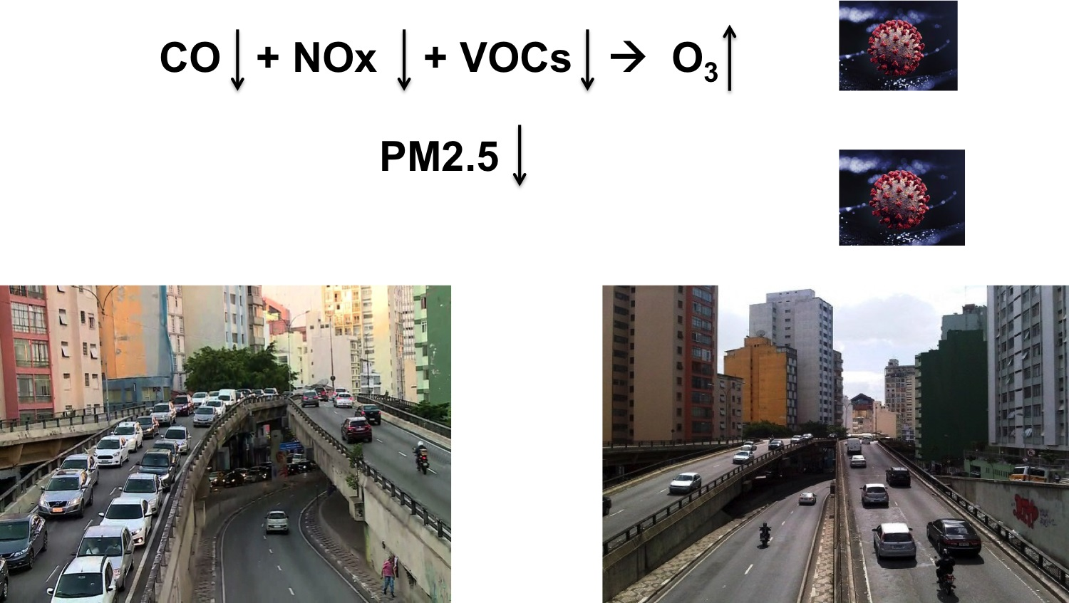
Owing to the lockdowns imposed during the COVID-19 pandemic, the number of vehicles circulating in large cities has fallen considerably. With fewer vehicles on the roads and companies operating at a reduced capacity, there has been a reduction in the emissions of nitrogen oxides (NOx), carbon monoxide (CO), volatile organic compounds (VOCs), and carbon dioxide (CO₂₎ in the atmosphere. The transport sector is an important emission source of air pollutants and greenhouse gases in the Metropolitan Area of São Paulo (MASP), where there is a fleet of around 7 million vehicles. In the MASP, both mobile and fixed sources were responsible for atmospheric emissions of approximately 120, 35, 70, 5, and 7 thousand tons of CO, VOCs, NOx, PM, and SOx, respectively, in the year 2019. Of these totals, 97%, 75%, 62%, 16%, and 40% of CO, VOCs, NOx, Sox, and PM, respectively, came from vehicular emissions, according to the CETESB Report of the Environment Agency of the State of São Paulo [1].

On 11 March 2020, the World Health Organization (WHO) declared COVID-19—a disease caused by the new Coronavirus SARS-CoV-2—a global pandemic [2]. In Brazil, the first case of COVID-19 was confirmed on 26 February 2020, in the state of São Paulo. By the end of 2021, there had been 22.2 million confirmed cases in Brazil, the majority being reported in São Paulo, i.e., of 4.4 million confirmed cases [3], it had the highest number in the country (i.e., 976,918) [4].

Brazil declared COVID-19 a public health emergency on February 3 [5], and São Paulo and Rio de Janeiro were the first states to impose social restrictions and encourage social isolation. On 24 March 2020, the partial lockdown was imposed by the São Paulo State government, which involved the closure of shopping malls, restaurants, gyms, elementary schools, high schools, and universities. Restrictions were introduced involving social distancing in supermarkets and drugstores, and a reduced schedule for public transport services, in addition to the adoption of a ’work at home’ office system, when possible. Thus, the interruption or reduction of several activities that might potentially cause pollution could mitigate the effects of air pollution on the health of the general public [6].

In terms of public health, a reduction in air pollution is directly proportional to a fall in the number of people with respiratory problems. In the wake of the lockdown brought about by the COVID-19 pandemic, fewer people suffered from respiratory problems, such as asthma, bronchitis, allergies, or cardiorespiratory diseases. The benefits to health brought about by the absence of sources of airborne contaminants underline the need to determine the nature of these pollutants in the atmosphere.

Moreover, the pollutants emitted by a certain country or locality are not restricted to the particular region in which they originate; they can cause damage beyond its borders. According to the World Health Organization (WHO), 92% of the world’s population lives in regions where air pollution levels exceed the limits laid down in its guidelines. About four million deaths per year can be attributed to exposure to the effects of air pollution on the environment, with 90% of them occurring in low- and middle-income countries. The Global Burden of Disease Study (2015) shows that air pollution is directly linked to 19% of deaths from cardiovascular disease worldwide, 24% from ischemic heart disease, 23% from lung cancer, and 21% from strokes [7].

Atmospheric chemistry plays a crucial role in the spread of radioactively active gases and aerosols [8]. In addition, climate variability and its patterns strongly influence atmospheric chemistry and air quality [9]. Owing to the non-linear behavior of chemistry and the important regional variations of emissions, it is essential to study the evolution of trace gases through remote sensing and compare them with observations from ground stations, measurements carried out by aircraft, and state-of-the-art models [10].

Air quality monitoring by satellite is carried out to estimate emissions, track pollutant plumes, ensure air quality, make forecasts of climate change, highlight extreme meteorological events, monitor long-term regional trends, and validate the data of the air quality models [10].

There is currently a wealth of atmospheric composition satellite data for air quality (AQ) applications that have proven to be valuable to environmental professionals: NO₂, SO₂, NH₃, CO, some VOCs such as formaldehyde and glyoxal, and aerosol optical depth (AOD), from which surface particulate matter (PM2.5) can be inferred [10].

The use of remote sensing in air quality studies has still only been explored to a limited extent, but is of great potential value, since some environmental satellites, such as TERRA (through the MOPITT sensor (CO) and (CH₄), MODIS and MISR (AOD), AQUA with AIRS sensor and the TANSO-FTS sensor on board the GOSAT satellite), have served as alternative and supplementary tools for monitoring the emission of pollutants. These tools have global coverage and provide the public with information on atmospheric composition and surface attributes [11,12,13,14,15,16,17].

A study carried out by the University of Toronto (UT) found that there was a 40% reduction in air pollution in cities that declared a state of emergency in February 2020, i.e., Wuhan, Hong Kong, Kyoto, Milan, Seoul, and Shanghai. This study, which was conducted by Marc Cadotte of UT, analyzed the air quality index (AQI) for each of the six cities affected by COVID-19 that introduced emergency measures in February 2020 [18]. The authors compared the 2020 AQI in these cities with that of February 2019 and found that all six cities showed a significant reduction in air pollutant concentrations during this year. However, in the case of the O₃ concentration in MASP, there was a 30% increase, which was probably due to a 77.3% decrease in NOx concentration, according to a study carried out in São Paulo [19]. Compared with the figures for previous events that had recently taken place in Brazil, such as the truck drivers’ strike between 21 and 31 May 2018, and also compared with the average for the same period from 2015 to 2017, there was a 31% decrease in CO, 38% in NO, and 31% in NO₂, but an increase in O₃ of 65% [20]. This increase in ozone can be attributed to the fall in NO levels, which react with O₃ to form NO₂ and O₂, the main consumption path of tropospheric O₃. The [21] study on the truck drivers’ strike, which examined 7 stations in the MASP over a period of four years, found a 50% reduction in the averages of CO and NO and a 40% increase in O₃, while the results for NO₂ and PM were mixed—which suggests sources other than vehicular are important, such as secondary reactions and the movement of pollutants from surrounding regions.

Improvements in air quality, which are linked to social distancing measures and a resulting reduction in vehicular traffic, have been reported in recent research. In Bangladesh, air pollutant data from a NASA satellite was used to make maps, and this was supplemented by Air Quality Monitoring Station (AQMS) data to assess air pollution during the pre-lockdown, lockdown, and post-lockdown periods of the COVID-19 pandemic. As a result, considerable improvements in a wide range of air quality parameters such as NO₂, O₃, CO, SO₂, PM2.5, PM10, AOD, and black carbon emissions were observed during the lockdown period [22]. For example, [23] relied on the Copernicus Atmosphere Monitoring Service to analyze fine particulate matter (PM2.5) data in China and observed a reduction of approximately 20–30% in February 2020 (monthly average) compared with monthly averages for February 2017, 2018, and 2019. The authors of [24] made use of the Copernicus Tropospheric Monitoring Instrument and data from a traffic station in Barcelona (Spain), provided by the local air pollution monitoring service, to assess changes in air quality during the lockdown in the city of Barcelona. They observed a reduction of 31% and 51% of PM10 and NO₂, respectively, during the lockdown compared with the month before the lockdown. The authors of [25] also analyzed local data from different regions of India to assess the effects of lockdowns on air quality. The authors observed a 43% and 31% reduction in PM2.5 and PM10, respectively, during the lockdown compared with the same period in the preceding four years. Other global regions showed a reduction in pollutants during the lockdown. For instance, on the basis of satellite data, it was found that NO₂ and AOD were reduced by approximately 20% during the lockdown in 2020 in India, in comparison with the figures for the previous five years (2015–2019) [26], while there was also a reduction in PM2.5 and NO₂ ground-based observations for the same period in seven Indian cities (except Mumbai, central India).

In the case of different regions of Poland, including urban areas and background sites, the PM2.5 and NO₂ during 2020 were lower (from 15 to 20% and from 18 to 30%, respectively) than the 10-year average [27]. On the basis of data from Sentinel-5P and Himawari-8, there were considerable changes in NO₂, HCHO, SO₂, CO, and AOD in many Asian cities from February 2020 to the previous year [28]. NO₂ decreased from 4% to 83%, and AOD decreased by 62%. The authors also showed that meteorological weather conditions could not explain the main variations in the pollutants. In the metropolitan area of Toronto, Canada [29], the levels of NO₂ decreased by approximately 35 to 40% during March and June 2020 compared with the previous 7 years, particularly within the region of the airport.

The variation in meteorological parameters and the relationship with the spread of daily cases of COVID-19 (from 1 April to 30 September 2020) in the four Indian megacities Delhi, Mumbai, Pune, and Ahmedabad, which differ in their climatology, were observed in the study by [30]. It was noted that weather variables such as relative humidity and absolute humidity showed a moderate positive correlation with daily COVID-19 cases in three cities (Delhi, Mumbai, Pune). There was a weak correlation between atmospheric temperature in Ahmedabad and Delhi, and a negative correlation was observed in the hill of Pune and the coast of Mumbai, which indicates that the lower temperature increased transmission. PCA analysis in this work revealed that COVID-19 cases are closely correlated with humidity [30].

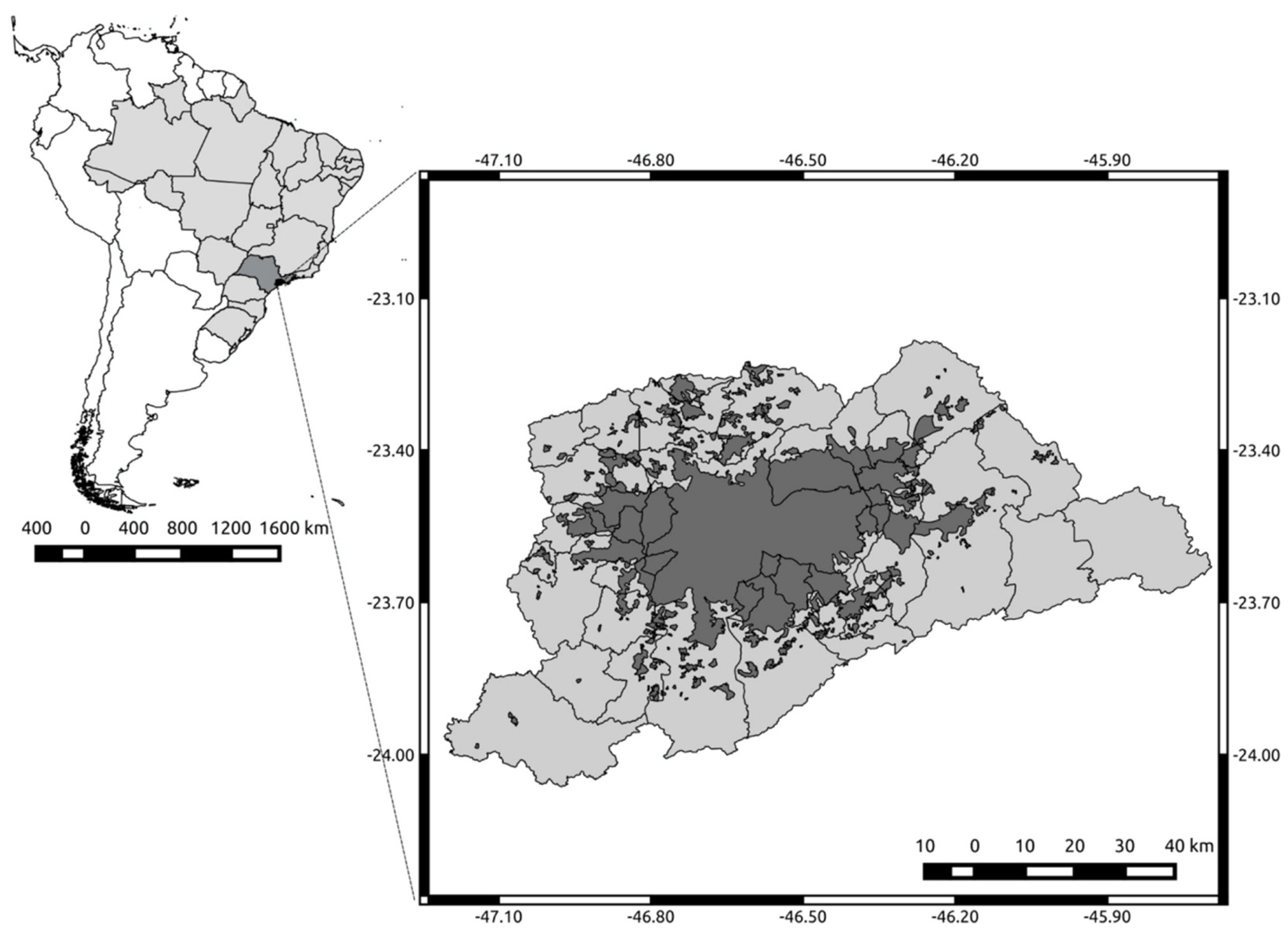
The aim of this study was to assess how far the partial lockdown affected the air quality in the MASP, which is the largest metropolitan region in Brazil, with around 22 million inhabitants, and one of the ten most populous metropolitan regions in the world. The lockdown was imposed to ensure that the necessary social distancing required by the COVID-19 pandemic was maintained. The analysis of CO, NO, NO₂, O₃ and PM2.5 pollutants was conducted by means of diurnal cycles from the lockdown period in April and May 2020, and the findings were compared with the average for the same period in the three previous years (2017–2019), when there was no pandemic. Meteorological data for the same period for MASP were also analyzed to determine the role of weather conditions in the concentration of pollutants within the context of the pandemic. These were supplemented by pollution maps, which were designed on the basis of data from the OMI sensors and MERRA-2 reanalysis for the south-east region of Brazil.

2. Materials and Methods

2.1. Characterization of the Study Area

The southeast region of Brazil is the second-smallest region in the country in area, and is only larger than the south region. The actual area encompasses approximately 924,620 km², 1/10 of the territory of Brazil. It includes four States: Espírito Santo, Minas Gerais, Rio de Janeiro, and São Paulo. It is the most developed region of the country and is responsible for 55.2% of the gross domestic product (GDP) of Brazil. São Paulo, Rio de Janeiro, and Minas Gerais lead in terms of nominal GDP. In terms of GDP per capita PPP, the southeast has the highest among all the Brazilian regions: USD 17,677.19 per annum. Three states are among the top five with the highest GDP per capita in Brazil, namely, São Paulo (2nd), Rio de Janeiro (3rd), and Espírito Santo (5th), eight among the top ten municipalities across the country, and three among the top four Brazilian capitals, Vitoria (1st), São Paulo (3rd), and Rio de Janeiro (4th). It contains the most populous municipalities, the highest population density, the largest iron ore deposits, the largest road-rail network, and the largest port complex in Latin America. It is the most important industrial, commercial, and financial region of the country. It employs 80% of Brazilian workers and consumes 85% of the total electricity generated in Brazil [31].

The state of São Paulo and the Metropolitan Area of São Paulo (MASP) are situated in the south-east region (Figure 1). The MASP is the largest metropolitan area in Brazil, with around 22 million inhabitants, and is one of the 10 most populous metropolitan regions globally. It brings together 39 municipalities in the state of São Paulo in a huge conurbation. According to the census compiled for July 1, 2022, the population was 22,048,504. This is greater than several countries in the world, such as Chile (17,248,450), the Netherlands (17,100,475), and Portugal (10, 487289) [31].

The area of the MASP—7946 square kilometers—corresponds to less than one-thousandth of the Brazilian territory and just over 3% of the territory of São Paulo. It has approximately the same dimensions as some nations, such as Lebanon (10,452 km²) and Jamaica (10,991 km²), and is larger than those of countries such as Luxembourg (2586 km²) [31].

The urbanized area comprises 2200 square kilometers. Between 1962 and 2002, the urban area increased from 874 km² to 2209 km². The metropolis suffers from the negative effects of conurbation, which deprive cities of their physical limits—owing to the unchecked growth of the urban area of MASP towards neighboring cities—giving rise to a continuous urban sprawl [31].

In practice, the MASP has a high-altitude humid climate (CWA), but many believe it to be of the subtropical type because most of this area is located a little south of the Tropic of Capricorn. Its topography and proximity to the sea (a distance of about 70 km) are the main factors that influence the climate of this immense metropolitan region. The Cold Fronts that come from the ocean rise from both below and above the plateau where they reach the southern escarpment of the MASP facing the wind, which carries moisture throughout the region. The relief conditions above an altitude of 760 m cause a sharp fall in temperature, especially during the night [32,33].

Thus, this region can be considered subtropical on account of its geographical location south of this tropic. The entire MASP has a subtropical climate of a CWA type, with dry and moderately cold and mild winters by Brazilian standards, and humid and relatively hot summers, with temperatures that rarely exceed 35 °C and in very rainy conditions [33].

In general, the MASP climate in the summer is hot and rainy, and in the winter it is mild and semi-arid, with slight variations in temperatures in different regions, and the climatic conditions can be either mitigated or worsened by the presence of factors that create microclimates. Between the different towns and cities of the MASP, these climates are only differentiated by the presence of greener or higher areas, or their proximity to the cliffs of the Serra do Mar, which exposes some municipalities in the south of the Metropolitan Area to humidity from the sea [32,33].

The MASP is the largest financial hub of the country and a center for the control of private capital, since it is the region where the Brazilian headquarters of the most important industrial, commercial, and, in particular, financial services are based [34].

This has given rise to a number of advanced services in the metropolitan region that rely to a great extent on the circulation and dissemination of information: planning, advertising, marketing, insurance, finance, and consulting services, among others. The region had a gross domestic product (GDP) of ZAR 760.04 billion in 2011, when it represented 56.32% of the GDP of the state of São Paulo [34].

São Paulo is the fourth most congested city in the world and second only to Los Angeles, Moscow, and New York. The inhabitants of the MASP spend an average of 2 h a day commuting to work, which leads to health problems and financial losses that can run into billions of dollars [35].

2.2. Air Pollution Data

In this research, the air pollutant concentrations originate from different sources and can be measured using different data, such as NO₂ near the surface, which was calculated by the OMI sensor, and CO, SO₂ and BC data, which were downloaded by the MERRA-2 to assess the monthly averages in the southeast region of Brazil. This has four states (namely, São Paulo, Rio de Janeiro, Espírito Santo, and Minas Gerais), accounts for 42% of the country´s population, and has two mega-metropolises, namely, São Paulo and Rio de Janeiro. The monthly averages for the period April and May 2020 (during the pandemic) were compared with the same period for the years 2017 to 2019 (pre-pandemic). Data from OMI and MERRA-2 were obtained from https://giovanni.gsfc.nasa.gov/giovanni/, (accessed on 1 November 2021), and the pollutant concentration figures were obtained with the aid of NCAR’s NCL.

2.2.1. NO₂ from OMI

In this study, the product of global NO₂ level 3 and grid (0.25 × 0.25 degrees) (OMNO2d) was used. The OMNO₂d Level 3 data product is good quality pixel-level data, which is grouped and average into 0.25 × 0.25 degrees global grids. This product contains the total column and the total tropospheric column of NO₂ for all atmospheric conditions and for sky conditions in which the cloud fraction is less than 30%. The data for the tropospheric column with a cloud fraction of less than 30% were used in this study.

OMI is a nadir viewing spectrometer covering a spectral region of 264–504 nm, which has been making atmospheric chemistry measurements in the 420–630 nm band since 2004 aboard NASA’s Earth Observation System (EOS)—Aura satellite. Aura completes a sun-synchronous polar orbit (altitude 705 km), with an ascending local equator crossing time (LECT) at 1:45 p.m. The OMI observations provide complete global coverage in a single day with a nominal ground footprint of 13 × 24 km² at the nadir. It measures various pollutants such as NO₂, SO₂, BrO, HCHO, and aerosols [36].

2.2.2. CO, SO₂, and BC from MERRA-2

CO, SO₂, and BC concentration data from MERRA version 2 (MERRA-2) were used. Atmospheric reanalysis produces long-term records of high global spatial and temporal resolution of meteorological fields and composition of the Earth’s atmosphere by employing data assimilation methodology, in which satellite and terrestrial observations are combined with the global circulation model (GCM) simulations in a statistically optimal way [37]. The Modern Era Retrospective Analysis for Research and Applications was the first reanalysis conducted using the Goddard Earth Observing System (GEOS) and the Data Assimilation System (GEOS) recommended by the Global Modeling and Assimilation Office (GMAO) from NASA. MERRA, first released in 2009, covered the years 1979 to 2015 (production ended 29 February 2016) [38]. This was followed by the MERRA version 2 (MERRA-2) dataset that was used in this work.

2.2.3. Data from the Monitoring Network of the Environmental Agency of the State of São Paulo (CETESB)

Measurements of hourly concentrations of pollutants were obtained at http://qualar.cetesb.sp.gov.br/qualar/home.do for the years 2017 to 2020, accessed 1 July 2021, from six AQMS in the MASP, namely, Grajaú-Parelheiros, Ibirapuera, Itaim Paulista, Parque Dom Pedro, Pinheiros, and São Caetano do Sul. The purpose of this was to characterize atmospheric pollution in different land use/emission conditions, by following WHO classification criteria on urban land use and exposure conditions [39]. The sites were classified as suburban residential, vehicular commercial, residential, and urban background by CETESB, and represented different conditions within the megacity. The World Health Organization states that decision-makers must include different types of urban land use and locations when creating an air quality network in a given area to collect information on how far the public is exposed to air pollution, i.e., the air within the city and its suburbs. Assistance is also given by the different spatial representations of the different monitoring sites [39,40,41].

Table 1. Categories of land use defined by the WHO and in the location of AQMS.

Station	Categories of Land Use	Latitude (South)	Longitude (West)
Grajaú-Parelheiros	suburban/residential	−23.78	−46.69
Ibirapuera	Background (urban)	−23.59	−46.65
Itaim Paulista	Residential	−23.50	−46.42
Pinheiros	vehicular/commercial	−23.56	−46.70
Parque Dom Pedro	Vehicular/commercial/	−23.54	−46.63
São Caetano do Sul	Residential	−23.62	−46.56

shows the four categories of urban land use that were used in this study, which were classified by CETESB in accordance with the criteria outlined above, together with the identification of the main circulation routes and vehicular traffic around the monitoring points, using the cited documents [39]. The aerial images showing the different features of each AQMS where data were used for this study are shown in Figure 2.

The hourly averages corresponding to the months of April and May were calculated for each of the monitoring stations in the MASP, and resulted in daily cycles (24 h) of pollutants, which allowed an investigation to be carried out of the impacts of concentrations on the region, and involved two diurnal cycles: pre-pandemic between April and May (2017–2019) and the same period that experienced the partial lockdown (2020) during the pandemic. In addition, changes in mean average concentrations were calculated to assess the relative change (%) compared with the period of partial lockdown during the pandemic (April and May 2020, hereafter called PL) with the monthly pattern of the pre-pandemic period (April and May of 2017, 2018, and 2019, hereafter PPP). Diff% is the percentage increase or decrease in the concentration of a given pollutant during the pandemic (April and May 2020) compared with the same period of the three previous years (2017, 2018, and 2019), as expressed in Equation (1):

$$\mathrm{diff}\%=\left(\left(\mathrm{PL}-\mathrm{PPP}\right)\ast 100\right)/\mathrm{PL}$$

(1)

where PL is the average hourly concentration from midnight to 11 p.m. during the months of April and May 2020 (pandemic), and PPP is the average hourly concentration from midnight to 11 p.m. during the months of April and May 2017, 2018, and 2019 (pre-pandemic).

2.3. AOD Data

AOD data (550 nm) were obtained from MERRA-2, which assimilates ground station aerosol data from AERONET and space aerosols from the Advanced Very High Resolution Radiometer (AVHRR), Multi-Angle Imaging Spectrum Radiometer (MISR), and MODIS [42,43]. The temporal resolution used for the MERRA-2 AOD data is monthly and the spatial resolution of the data is 0.625 degrees × 0.5 degrees.

Observational data of the AOD parameters obtained from AERONET measurements in São Paulo (23° S 46° W) were also used. Data from AERONET were obtained from https://aeronet.gsfc.nasa.gov/cgi-bin/draw_map_display_aod_v3, (accessed on 1 October 2022). AOD is a key parameter in aerosol measurements, as it is a measure used to quantify the amount of aerosols present in the atmospheric column [44]. AERONET measurements are obtained through the use of solar photometers and are site-specific. Measurements are carried out at various wavelengths and are timed at 15 min intervals with an accuracy of ±0.015 s. AERONET products are available at different processing levels: Level 1.0 (raw data), Level 1.5 (automated tracking data in the cloud), and Level 2.0 (quality assured data). In this work, Level 2.0 data are used to eliminate cloud interference and ensure data quality.

The AOD measurements from AERONET stations are carried out at 500 nm, while the MERRA-2 AOD product is available at 550 nm. AERONET AODs at 550 nm are calculated using the Angström exponent available in the same instrument at 440–675 nm, as expressed in Equation (2):

$${\tau }_2=\frac{{\tau }_1}{e^{\left[-\alpha ln\left(\frac{{\lambda }_1}{{\lambda }_2}\right)\right]}}$$

(2)

where τ₂ is the AOD at 550 nm, τ₁ is the AOD at 500 nm, α is the Angström exponent between 440 and 675 nm, and λ₁ corresponds to 500 nm and λ₂ to 550 nm.

2.4. Meteorological Data

Meteorological parameters were downloaded from two stations, and we also used pollutant data, such as wind speed, relative humidity, and temperature. These parameters were only studied for the AQMS of Parque Dom Pedro and São Caetano do Sul, as they were not available for the other stations. Global solar radiation comes from the Parque Dom Pedro station. All the variables were analyzed during the pre-pandemic period between April and May (2017–2019) and the same period at the time of the partial lockdown (2020) during the pandemic.

Precipitation was collected during the pre-pandemic period between April and May (2017–2019) and the same period at the time of the partial lockdown (2020) during the pandemic by a rain gauge (QMR102, Vaisala) installed in the automated weather station of São Paulo (23.49° S, 46.62° W, and 786 m) from the National Meteorological Institute (INMET), https://portal.inmet.gov.br/, (accessed on 1 October 2022).

3. Results and Discussion

Significant improvements in air quality were observed in the urban area in light of the reductions in air pollutants monitored in areas that are highly influenced by vehicular traffic in MASP and MARJ, as shown in Figure 3, for NO₂ from the OMI sensor. There was a reduction in NO₂ concentrations from 10% to more than 60% in the MASP and MARJ, whereas the figure was around 10% in MABH and MAV. As Brazil is a country with 8.5 million km², the initial serious effects of the COVID-19 pandemic were felt in the states of São Paulo and Rio de Janeiro, and then spread to other regions of the country, particularly the more populous cities.

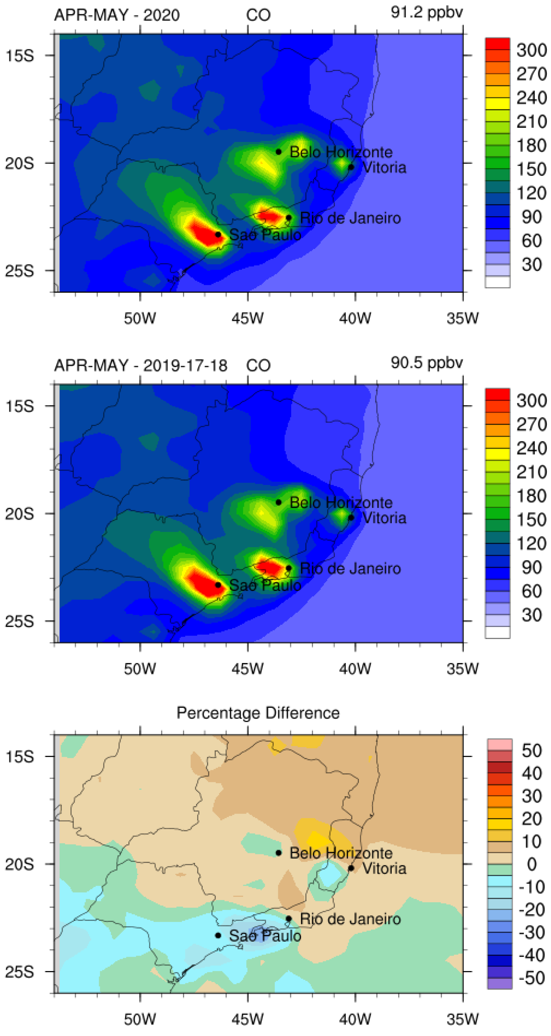
Figure 4 shows the CO near-surface concentrations from MERRA-2, where there was a CO decrease of around 10% during the pandemic over almost the entire São Paulo state, especially on the border between the states of São Paulo and Rio de Janeiro, where it was accompanied by a decrease in the traffic flow of both light and heavy vehicles in this region. Small changes in CO were observed in Belo Horizonte and Vitoria, which suggests that these cities were less affected by pandemic restrictions, largely because partial lockdowns were imposed in these localities for shorter periods than in other regions in São Paulo.

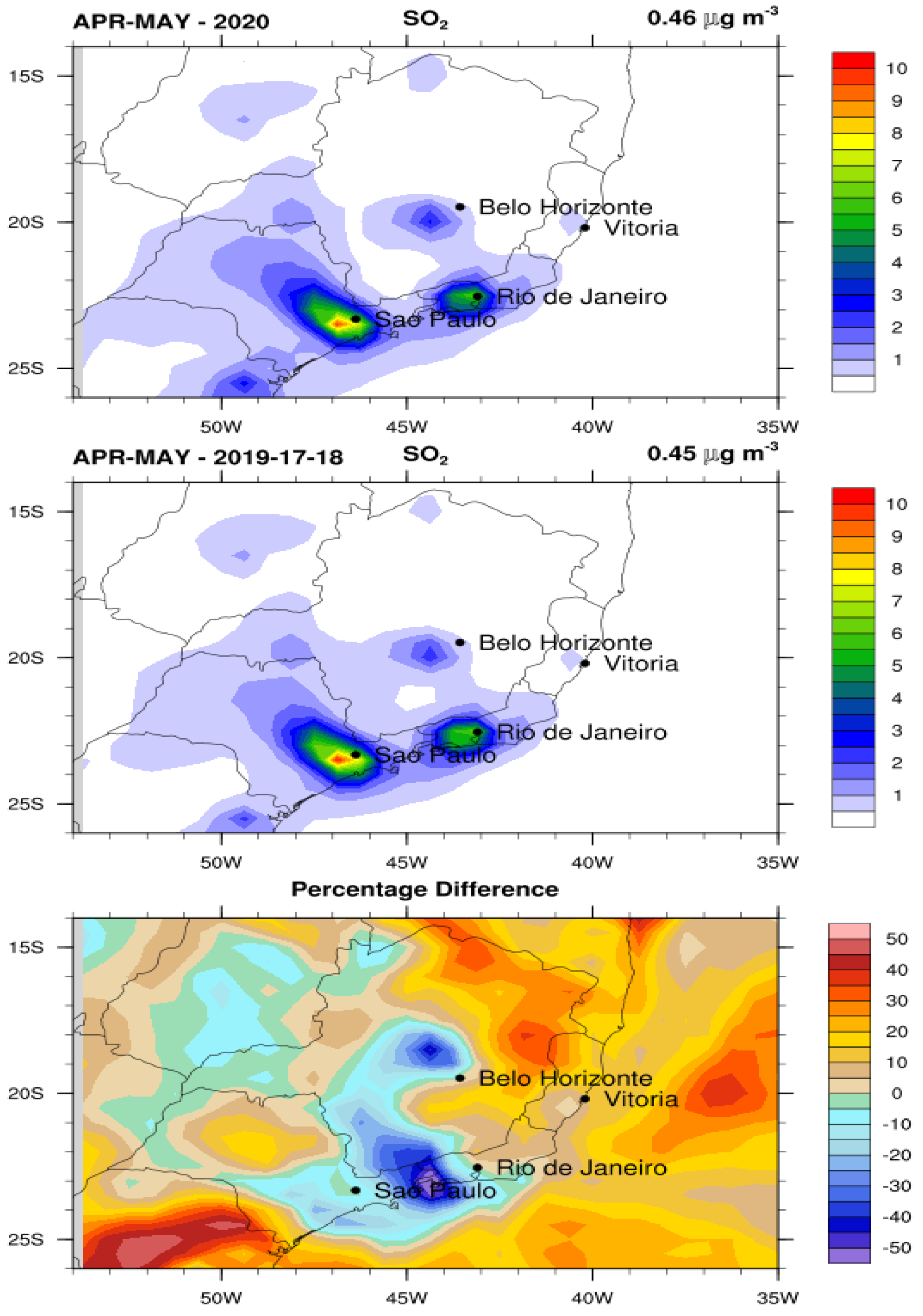
Figure 5 shows the SO₂ near-surface concentrations from MERRA-2, 5 to 10% lower SO₂ concentrations were found in the MASP and MARJ, and in the west of MABH, there was a decrease of 30 to 50% on the border between the states of São Paulo and Rio de Janeiro. There was an increase in the SO₂ pollutant in the MAV region during the period under study since the pandemic did not significantly affect the air quality.

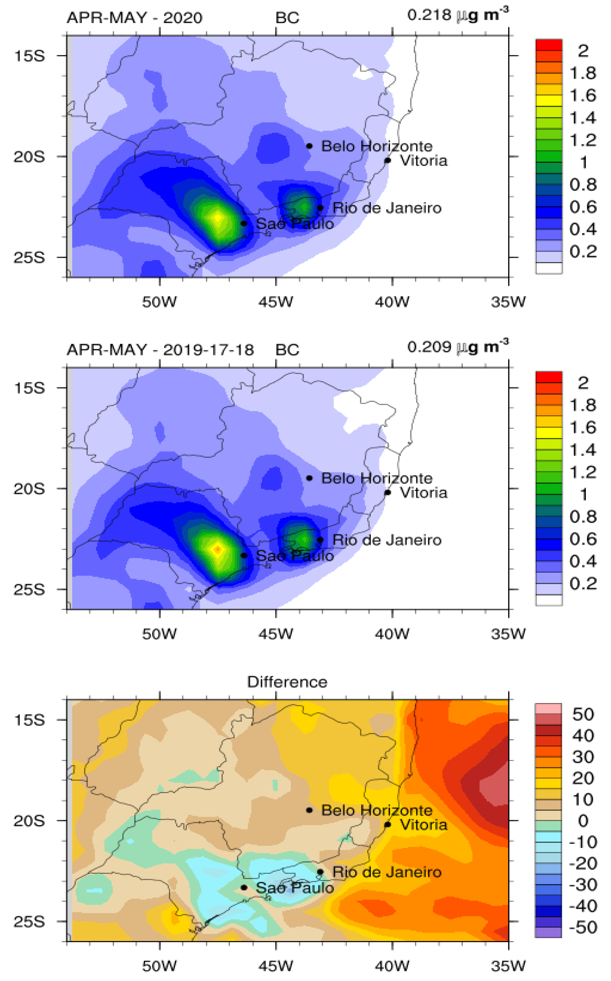
Figure 6 shows the surface BC concentrations from MERRA-2, with a 5–10% decrease in the MASP and on the border between the states of São Paulo and Rio de Janeiro, probably due to the reduction in diesel-powered truck traffic. In contrast, in the MABH and MAV, there was no reduction in this pollutant, mainly because, as stated earlier, these regions were less affected by the pandemic.

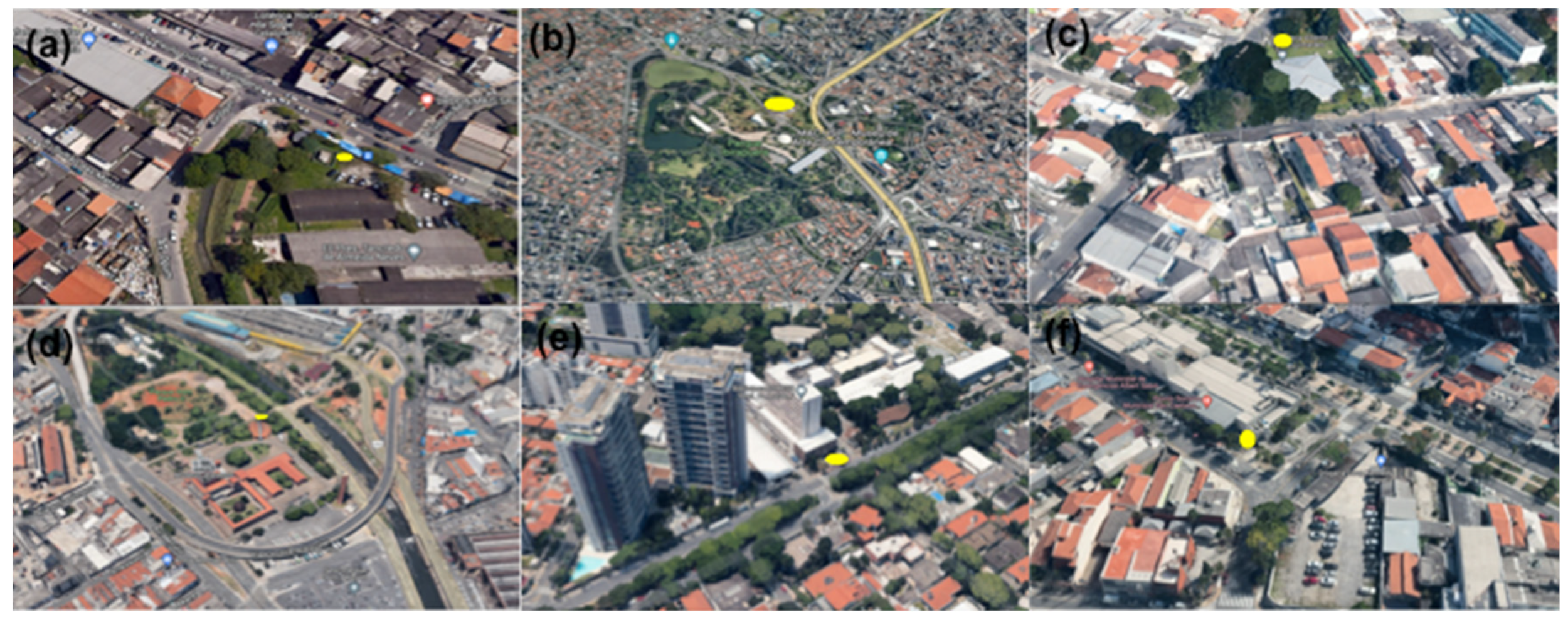
The meteorological parameters of the AQMS of Parque Dom Pedro and São Caetano do Sul were analyzed from the 6 MASP stations that were used to compare the concentration of pollutants at MASP, in April and May 2020 (pandemic) with the same period from 2017 to 2019 (pre-pandemic), since only these two stations have meteorological data for temperature, relative humidity, wind speed, and global solar radiation. The precipitation data were obtained from an INMET station close to these stations, where these meteorological variables and the pollutant concentration data were measured. Supplementary Figures S1–S5 show the difference in weather conditions during the period of this study (April and May 2020) with the same period in the previous three years (April and May 2017, 2018, and 2019). Figure S1 shows that the temperature during the April and May period of the pandemic in 2020 was lower in the two stations that measure this variable, while the hourly average air temperatures were 7.1% and 16.3%, which is lower than the same pre-pandemic period. Figure S2 shows the lowest relative humidity during the pandemic period (the hourly average for April and May 2020) compared with the pre-pandemic period (the same average period from 2017 to 2019), and the relative levels of humidity were 9.4% and 8.8% lower at the Parque Dom Pedro and São Caetano stations, respectively. Figure S3 shows that there was practically no significant variation in wind speed when the pandemic and pre-pandemic periods of this study were compared; at the São Caetano do Sul station, there was an increase in wind speed from 10 am to 14 pm. The wind speeds were 1.4% and 0.6% lower at Parque Dom Pedro and São Caetano stations, respectively. Global solar radiation was 14.3% higher at Parque Dom Pedro station, as shown in Figure S4. As can be seen in Figure S5, the total precipitation that occurred in the period of this study during the pandemic in April and May 2020 is the lowest recorded when compared with previous years (2017–2019), similar to 2018, but even lower in the other years. The slight difference in temperature, relative humidity, wind speed, and global solar radiation, as well as the considerable reduction in precipitation during the pandemic period compared with the prior period, indicate that the pollutant reductions observed during the pandemic period were not determined by changes in dispersion conditions.

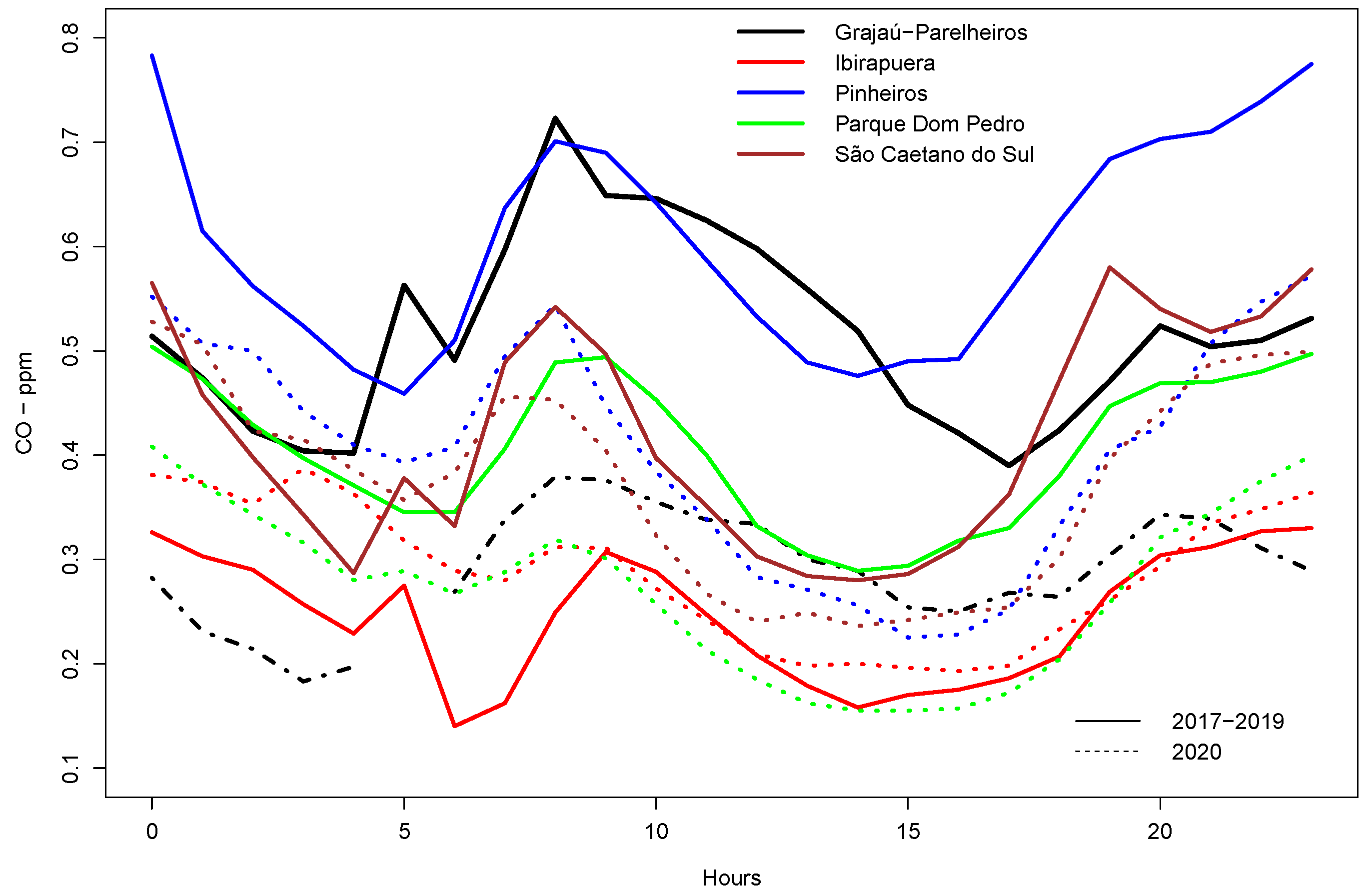
Figure 7 shows the hourly average rate of CO concentrations for April and May 2017, 2018, and 2019 (the pre-pandemic period) and for the same months in the year 2020 (during the pandemic) for 5 AQMS from MASP.

It can be seen in Figure 7 that the daily temporal pattern of CO concentrations did not change during the two periods. In the MASP, 97% of the CO emitted comes from vehicular emissions, which explains the increase in concentrations from 6:00 a.m. to 9:00 a.m., the time of greatest traffic density. After this time, concentrations decline, and there is an increase again from 5:00 p.m. to 8:00 p.m., which coincides again with the second peak of traffic in the MASP.

Figure 7 also shows an average reduction of 77.4%, 14.7%, 48.7%, 41.1%, and 12.1% in CO concentrations for the monitoring stations of Grajaú-Parelheiros, Ibirapuera, Pinheiros, Parque Dom Pedro, and São Caetano do Sul, respectively, as well as for the Ibirapuera station, where the campaign hospital specializing in COVID-19 care was located. The Ibirapuera station is located further away from the vehicular source of pollution; it is a region where primary pollutants have lower concentrations than stations near the main roads, although the secondary pollutant, O_3, is high in this location.

A study carried out using data from the CETESB AQMS in the city of São Paulo and Cubatão (on the southern coast of São Paulo State) compared data from the period of partial lockdown during April 2020 with the April monthly average of the previous five years (2015, 2016, 2017, 2018, and 2019) [19]. The study reported a decrease in CO concentrations of 53.1% and 64.8%, respectively, from measurements carried out in the city of São Paulo [19]. In another study carried out in the city of Rio de Janeiro, which compared 30 days from mid-March to the first half of April 2019 with the same period in 2020, there was a reduction of 38% and 36.4% in the concentration of CO in the regions of Bangú and Tijuca, respectively [45].

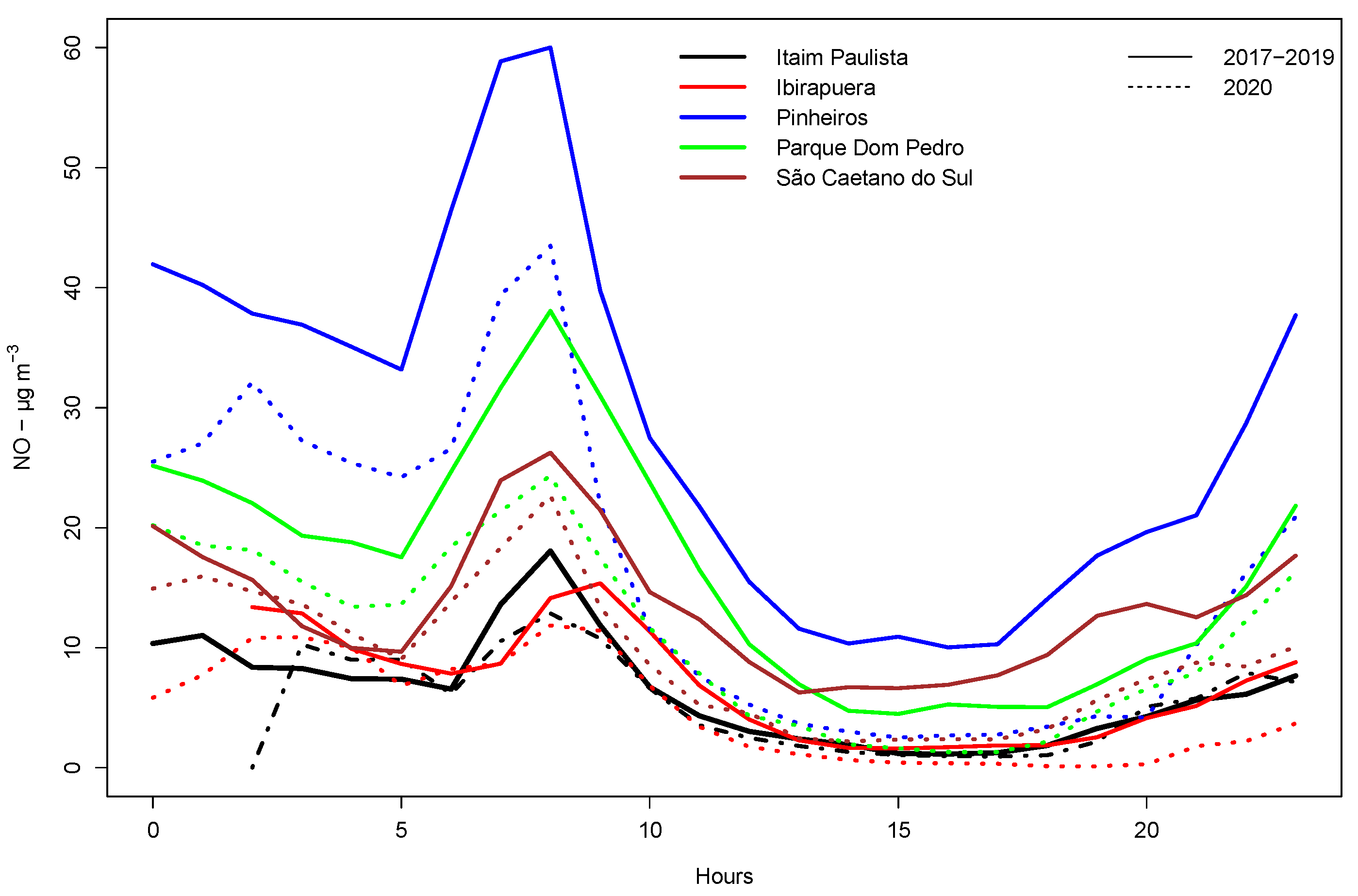
Figure 8 shows the hourly average NO concentrations for the April-May period for 2017, 2018, and 2019 (pre-pandemic) and the April-May period for 2020 (during the pandemic).

According to the results in Figure 8, the Ibirapuera station had a NO concentration reduction of 47.3% when compared with April-May for 2020 (during the pandemic) and April-May for 2017, 2018, and 2019 (pre-pandemic). It can be concluded from this that there was less diesel traffic near this station, since 48% of NOx emissions in the MASP come from heavy and diesel-fueled vehicles [46]. At the Itaim Paulista station, there was a reduction in NO concentrations of 19.2% compared with the average pre-pandemic level, as heavy vehicle traffic in this region is lower than in the other AQMS used in this study. At the Parque Dom Pedro and São Caetano do Sul stations, there was a reduction in NO levels of 37.0% and 45.5%, respectively. In the case of the Pinheiros station, there was a reduction in NO concentrations of 75.6%. In general, NO concentrations during the pandemic were lower, particularly at the Pinheiros and Parque Dom Pedro stations, which are close to roads with heavy traffic. Pinheiros station is close to one of the main roads in the city of São Paulo (Marginal Pinheiros) with a high rate of truck traffic, and Parque Dom Pedro station is close to an urban bus terminal that uses diesel fuel. Traffic emissions from heavy diesel vehicles are the primary source of NO [1,46,47]. The times with the highest concentration, both in the periods with and without a lockdown, were the peak hours of vehicular traffic, from 7:00 to 11:00 a.m. and from 7:00 p.m. onwards. This is when concentrations increase as a result of vehicular emissions but decrease at the height of the planetary boundary layer, owing to a lack of O₃ production at night (which consumes NO during the day).

A previous study using data from the CETESB AQMS in the cities of São Paulo and Cubatão (on the south coast of São Paulo State) compared data during the pandemic and pre-pandemic periods and found there was an increase in NO concentrations of 8% for Cubatão, where the largest Latin America industrial hub is located, with fertilizer, steel, chemical, and petrochemical companies, while at São Paulo city there was an average decrease of 75% in NO concentrations [19].

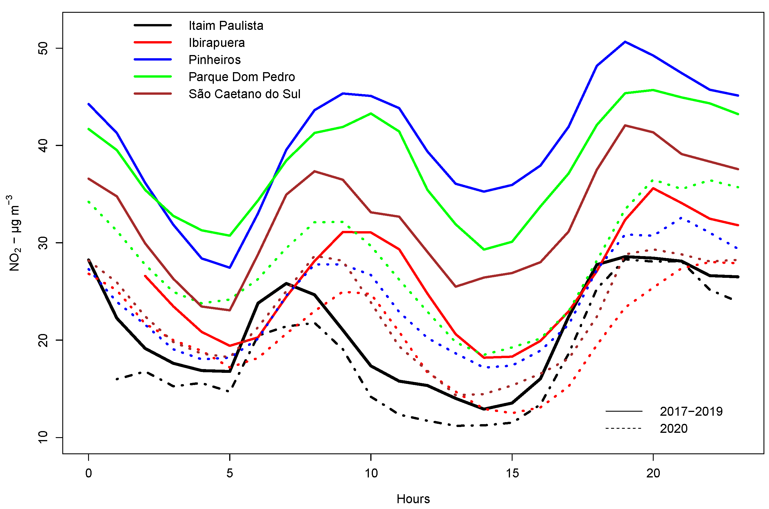
Figure 9 shows the NO₂ mean average hourly concentrations during the pandemic and pre- pandemic periods.

NO₂ concentrations were 21.6% lower at the Itaim Paulista station during the pandemic period. Parque Dom Pedro and São Caetano do Sul had a NO₂ reduction in hourly averages of 31.9 and 44.3%, respectively. Pinheiros station, located near a road with heavy vehicular traffic, had the highest NO₂ reduction in the lockdown period (69.6%).

Ibirapuera station had a reduction of 26.1%. There was an increase in NO₂ concentrations during the morning from 6:00 to 10:00 a.m. in both periods (i.e., during the pandemic and pre-pandemic periods), as a result of vehicular emission, but also secondary NO₂ was formed in the atmosphere through the oxidation of NO with O₃, and also by the oxidation of VOCs radicals with NO. NO₂ concentrations decreased from 12:00 to 16:00, which coincides with the period of higher O₃ concentration in the MASP. This period also had greater solar radiation, as it is the time when NO₂ is undergoing photolysis reaction, and forming NO and atomic oxygen. NO₂ concentrations increased again after 6:00 p.m., as this was the peak period of vehicular traffic.

A similar comparison was made by [19], for both periods, i.e., during the pandemic and pre-pandemic periods, when there was a decrease in NO₂ concentrations of 48.6% and 72.7% at two monitoring points in the city of São Paulo. Similarly, in the case of Cubatão, there was a reduction of only 5.6% in NO₂ concentrations [19], which underlines the importance of industrial sources of NOx. Hence, there was not the same fall in NO₂ concentration as during the truck drivers’ strike in the year 2018, which led to lower vehicle emissions, even when companies continued to operate [21].

In a study carried out in the city of Rio de Janeiro, which involved comparing the last half of March with the first half of April 2019 with the same period for 2020, there was an average reduction in NO₂ level of 27% and 24% in the region of Bangú and Tijuca, respectively [45]. The less significant NO₂ reduction with regard to CO and NO demonstrates its lower reactivity and underlines the importance of this pollutant’s secondary fraction in the MASP.

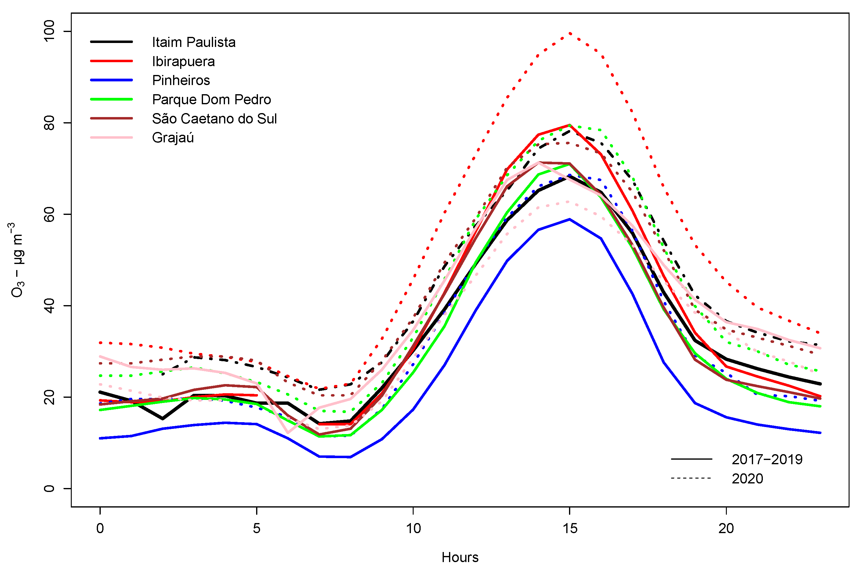
Figure 10 shows the mean average hourly O₃ concentrations during the pandemic and pre-pandemic periods. When both these periods are compared, there was an increase in O₃ concentrations of 27.3% in Ibirapuera, 21.5% in Itaim Paulista, 26.1% in Pinheiros, 21.1% in Parque Dom Pedro, 19.4% in São Caetano do Sul, and a reduction of O₃ of 19.5% at the Grajaú-Parelheiros station, an atypical behavioral pattern, since in the MASP, when NOx concentrations decrease, there is usually an increase in O₃ [21,48,49,50,51]. It would have been useful to have the NOx data for the Grajaú-Parelheiros station for further analysis, but there was no NOx-measuring device at this monitoring point.

The O₃ concentration starts to increase after 9:00 a.m. owing to the emission of primary pollutants and their precursors, such as CO, VOCs, and NOx, in the early morning hours, which coincide with the peak time of vehicular traffic. The formation of O₃ occurs later after the emission of primary pollutants and after the availability of sunlight, and reaches its maximum concentration from 1:00 p.m. to 3:00 p.m. At nighttime, O₃ is no longer formed due to the lack of sunlight, thus NO₂ is formed from NO (Reaction 3), which is a predominant traffic source, as this takes place in MASP. NO₂ and O₃ react to form NO₃ (Reaction 4). At nighttime, N₂O₅ can be formed through a reaction of NO₂ and NO₃ (Reaction 5) and decomposes at a rate coefficient k−3, and hence N₂O₅ [52,53,54].

NO + O₃ → NO₂ + O₂ → k₁

(3)

NO₂ + O₃ → NO₃ + O₂ → k₂

(4)

NO₂ + NO₃ + M ↔ N₂O₅ + M k₃ (forward), k₋₃ (reverse)

(5)

The reduced O₃ production is overwhelmed by the weakened nitric oxide (NO) titration resulting in a net increase of O₃ concentration. Although the reduction in emissions of NO increases O₃ concentration, it leads to a decrease in the Ox (O₃  +  NO₂) concentration, which is a sign of reduced atmospheric oxidation capacity on a regional scale. The dominant effect of NO titration underlines the importance of prioritizing VOCs [52].

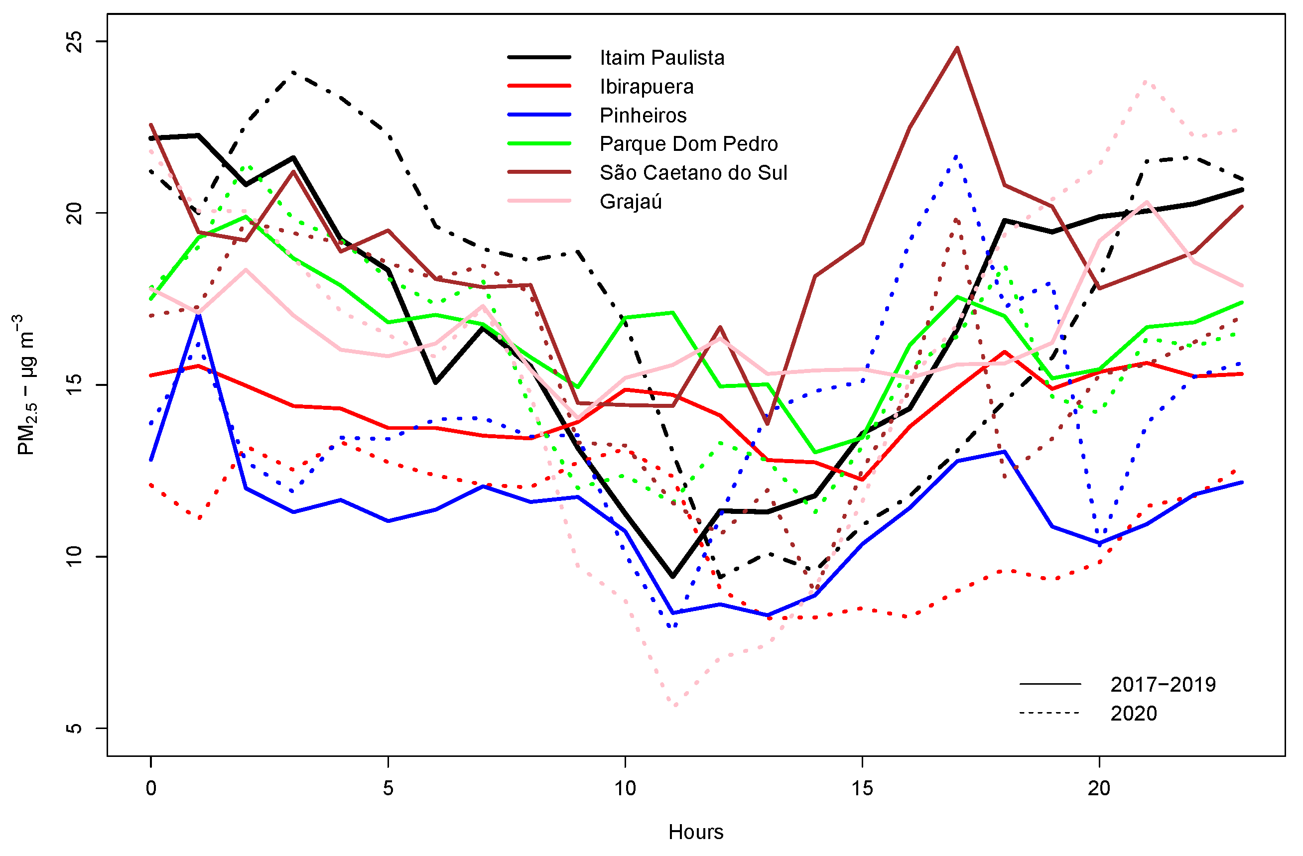
Figure 11 shows the mean hourly PM2.5 concentrations during and prior to the pandemic period. It was noted that PM2.5 behaved in a different way from CO, NO and NO₂ which had lower concentrations in practically all the air quality monitoring points in this study. PM2.5 had a reduced concentration at the Ibirapuera station at all times during the pandemic period. At the Itaim Paulista station, there was an increase in the PM2.5 concentration from 9:00 p.m. to 11:00 a.m. during the pandemic period, and then the concentration decreased from 12:00 p.m. to 8:00 p.m. At Grajaú-Parelheiros station there was a large decrease in PM2.5 from 9:00 to 15:00. At Pinheiros station, there was an increase in PM2.5 concentrations from 12:00 to 19:00 during the pandemic. At Parque Dom Pedro and Grajaú stations no quantitative differences were found between the pandemic and pre-pandemic periods. In light of the average level of PM2.5 concentrations, when both periods are compared, there was a reduction at the stations of Grajaú-Parelheiros (3.7%), Ibirapuera (30.1%), and São Caetano do Sul (20.7%). In the case of Itaim Paulista station, when the average of all the times is taken into account, there is no significant difference between both periods (just an increase of 2.9%), a decrease from 12:00 p.m. to 08:00 p.m. and an increase in concentrations from 09:00 p.m. to 11:00 a.m. With regard to the Parque Dom Pedro station, there was an average decrease of 4.6% during the pandemic period.

In Supplementary Materials Figure S6, there is a comparison between the AOD value of the AERONET station, located in the city of São Paulo, close to the AQMS (which used the pollutant concentration data provided in this work), and the MERRA-2 data. The AERONET versus MERRA-2 data from April and May (2017 to 2019—pre-pandemic) and the same period in 2020 (pandemic) show that the MERRA-2 data are underestimated when compared with the data from AERONET. When only the AERONET data are taken into account, the AOD value is 46% lower in the pandemic period than in the pandemic period, which is evidence that there was a reduction in the concentration of aerosols in the pandemic period.

On the basis of data obtained from six terrestrial air quality measurement stations, this work has shown that gases emitted by primary sources, such as CO and NO, decreased by 38.8% and 44.9%, respectively, in the period of April and May 2020 (pandemic), compared with the same period for 2017–2019. Additionally, NO₂ and PM2.5 were reduced by 38.7% and 6%, respectively, while O₃ increased by approximately 16% in the same period. The AERONET AOD values were 46% lower in the pandemic period than in the period without a pandemic. No significant changes in the meteorological variables could explain these pollution variations. The results showed that temperature, RH, and wind speed decreased by 11.7%, 9.1%, and 1%, respectively, during the pandemic period. Rainfall and global solar radiation were 7 times and 14.3% lower, respectively, for the pandemic period. Meteorological conditions could not explain the decrease in MASP pollutants, such as CO, NO, NO₂, PM2.5, as observed in Figure S5 during the period of this study from April and May 2020 during the pandemic. Compared with April and May of the three previous years without a pandemic (2017, 2018, and 2019), precipitation was 7 times lower during the pandemic than in the pre-pandemic period, so it was expected that there would be less precipitation since there was an increase in pollution in the pandemic period, but the opposite occurred even though there was much lower precipitation in the pandemic period. Otherwise, the lower number of people on the roads resulting from the partial lockdown could largely explain these anthropogenic reductions in emissions, mainly caused by vehicles. According to the Environmental Agency of São Paulo State (CETESB), the main MASP atmospheric pollutant emissions are from vehicle sources, which account for approximately 97%, 75%, 62%, 16%, and 40% of CO, VOCs, NOx, SOx, and PM, respectively. Thus, it is clear that a reduction in the use of vehicles could significantly affect the air quality of the study area.

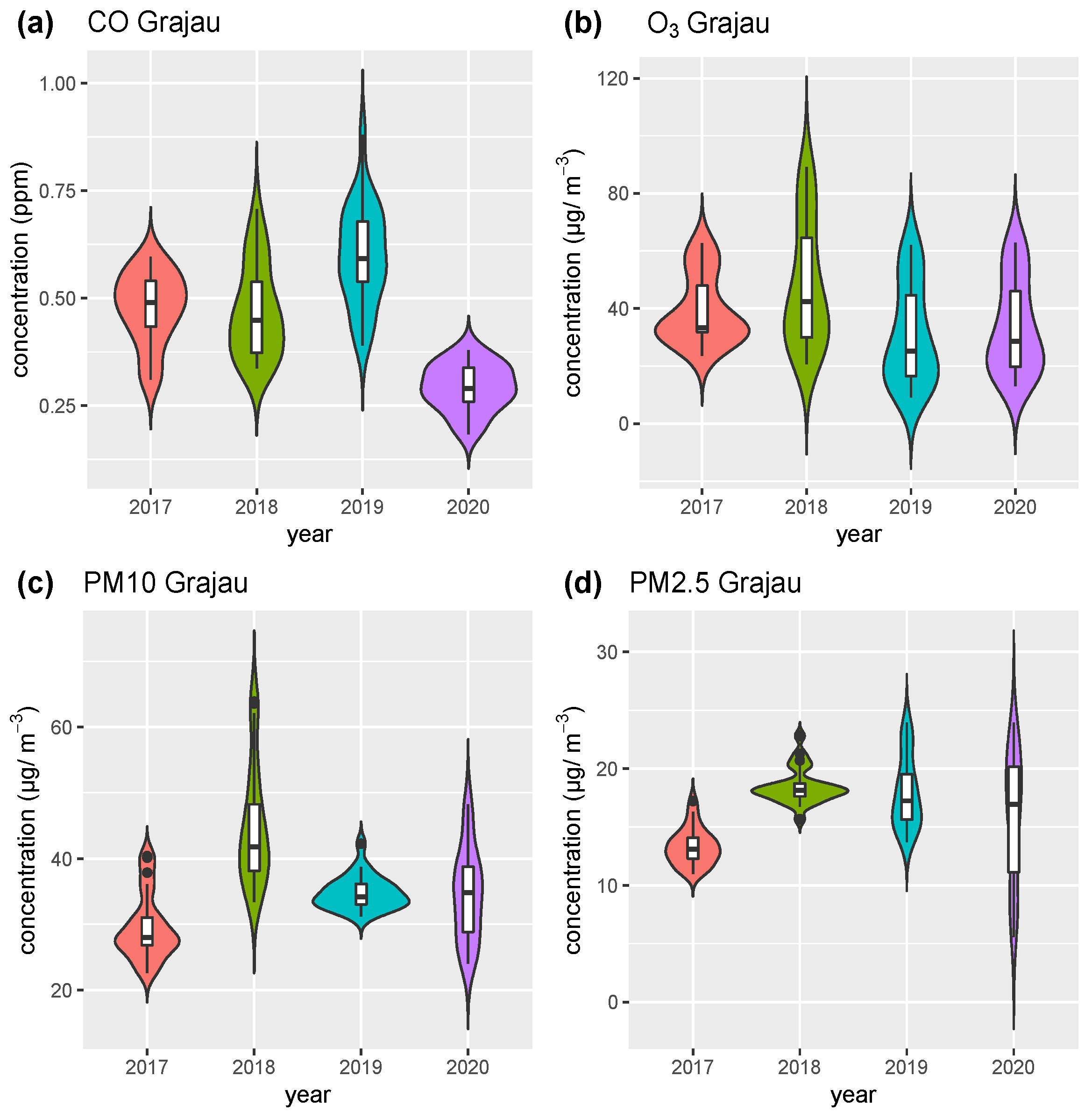
Figure 12a displays the violin graphs for Grajaú station from the four years studied for CO. The year 2020 during the pandemic period has the lowest median, with upper and lower limits and lower outliers than is the case in the pre-pandemic period. In the case of O₃ in Figure 12b, the median is slightly higher during the pandemic in the year 2020 than in the year 2019, but lower than in the years 2017 and 2018, whereas the data distribution is similar in the year 2020 when this is compared with the years 2017 and 2018. With regard to PM10 (Figure 12c), the year 2020 has a median similar to the year 2019, but a different distribution from the data in the year 2020, with higher upper and lower limits in the year 2020 than the years of the pre-pandemic period. In the case of PM2.5 (in Figure 12d), the year 2020 has a median similar to that of the years 2018 and 2019, but a different distribution of data, with higher upper and lower limits in the year 2020 than the years of pre-pandemic.

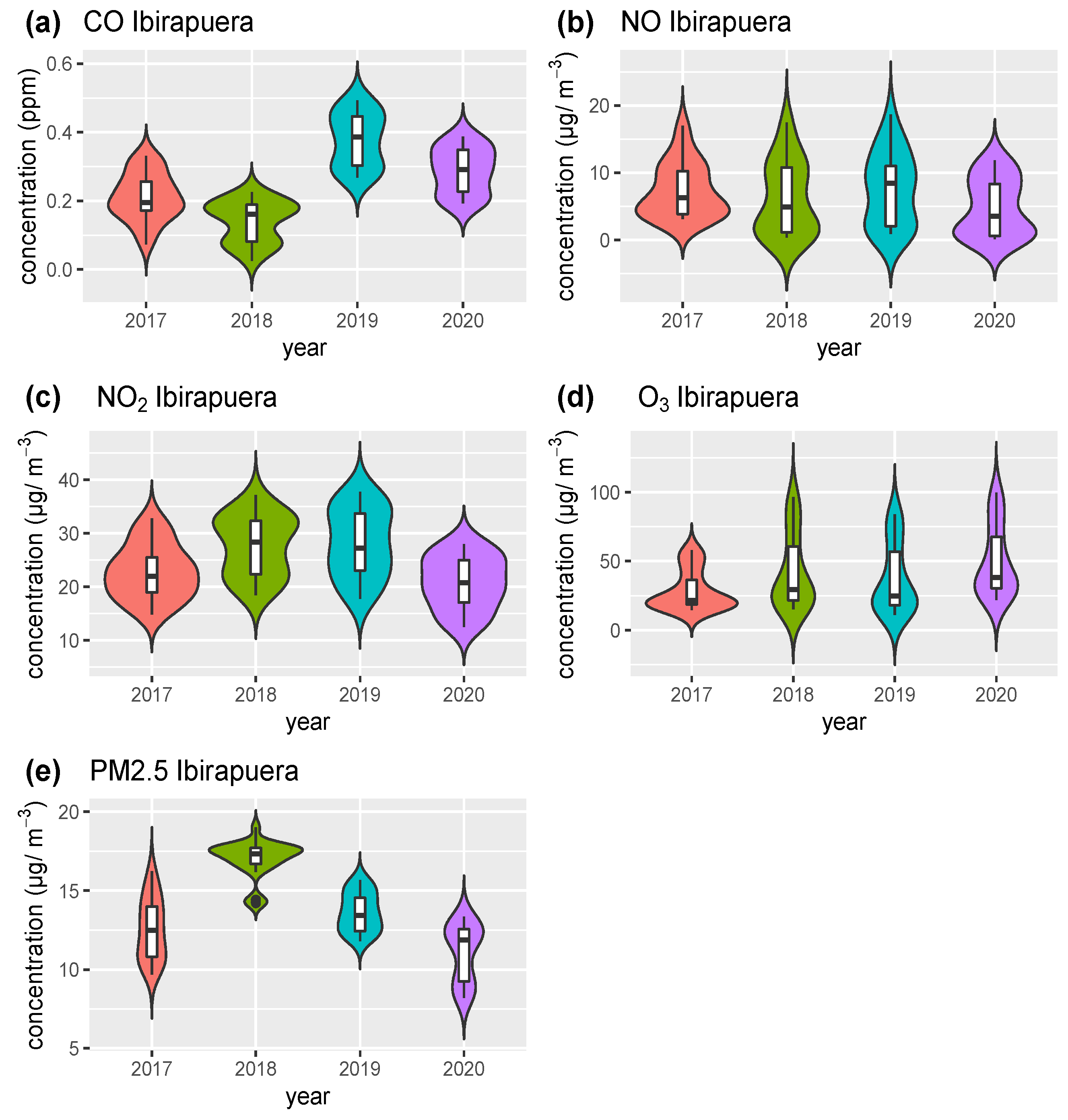
Figure 13 shows the violin graphs for the Ibirapuera station. In Figure 13a, during the pandemic (in 2020), CO has a median concentration lower than that in the year 2019, but higher than 2017 and 2018. With regard to NO and NO₂ (Figure 13b,c), there is a lower median concentration than in the pre-pandemic period (namely, 2017, 2018, and 2019). The median for O₃ during the pandemic period (2020) is higher than in the pre-pandemic period owing to a decrease in NO (in 2020), a pollutant that consumes O₃. PM2.5 is lower during the pandemic (2020) than in the pre-pandemic period.

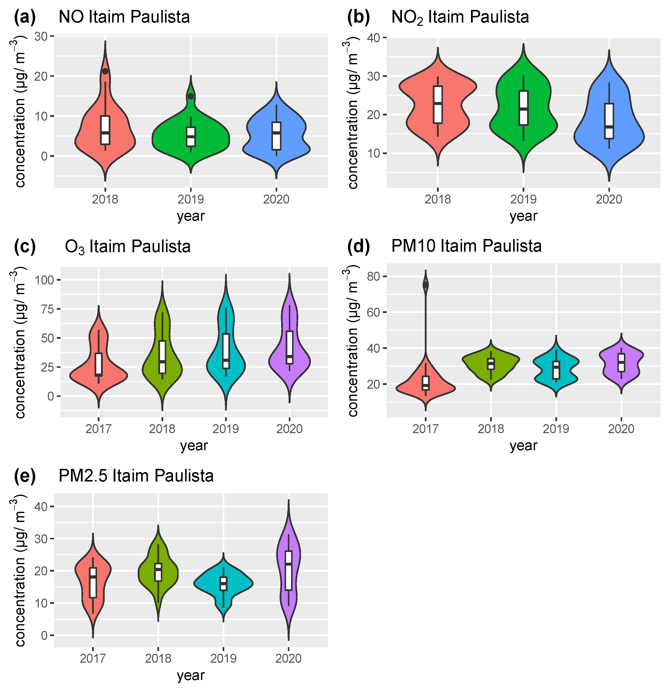
Figure 14 shows the violin graphs for the Itaim Paulista station. There is no significant variation in the concentration of NO, as shown in Figure 14a, compared with the pandemic year (in 2020) with the years 2018 and 2019. The NO₂ (Figure 14b) has a lower median concentration than in the years 2018 and 2019. On the other hand, O₃ (Figure 14c) has a slightly higher median concentration in the year 2020 compared with other years. The PM10 (Figure 14d) during the pandemic (in 2020) does not show any significant difference in the median concentration than in the pre-pandemic period (2017–2019). PM2.5 (Figure 14e) has a higher median concentration during the pandemic 2020 than the pre-pandemic period.

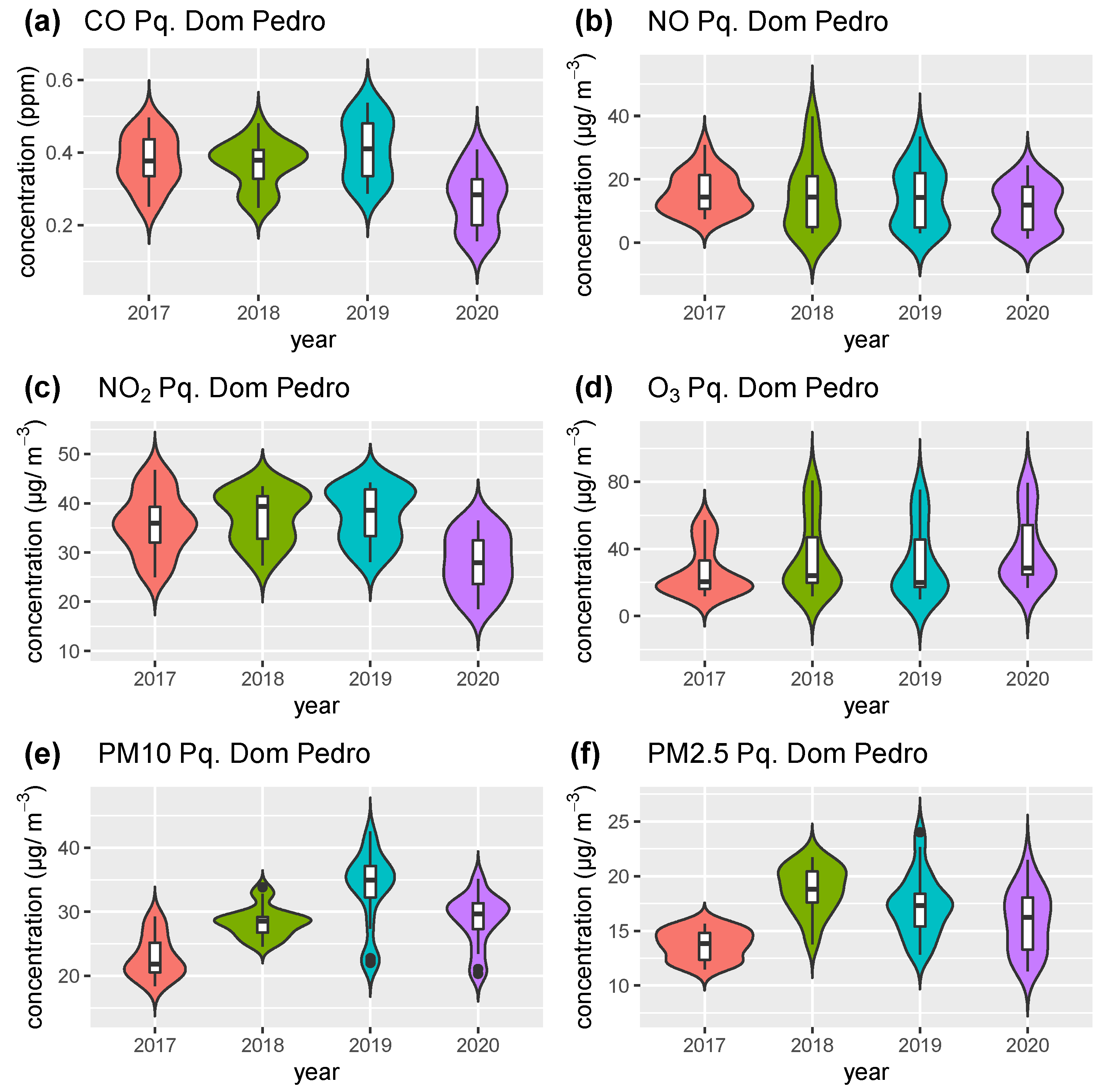
Figure 15 shows the violin graphs for the median of pollutants for the Parque Dom Pedro station. In Figure 15a for CO, the year 2020 of the pandemic has a lower median than in the pre-pandemic period, but the data distribution is similar for all the years. In Figure 15b, for NO, the median is similar during the pandemic (in 2020) to the pre-pandemic period. In Figure 15c, NO₂ has a lower median and lower limit during the pandemic than in the pre-pandemic period. In the case of O₃, Figure 15d indicates a slightly higher median during the pandemic than in the pre-pandemic period, but a similar data distribution for all the years of the study. In Figure 15 for PM10, the median is lower in 2020 than in 2019, but higher in 2017 and 2018. Figure 15f indicates that PM2.5 had a lower median in 2020, during the pandemic, than in 2018 and 2019, during the pre-pandemic period, and a lower limit during the pandemic period (in 2020).

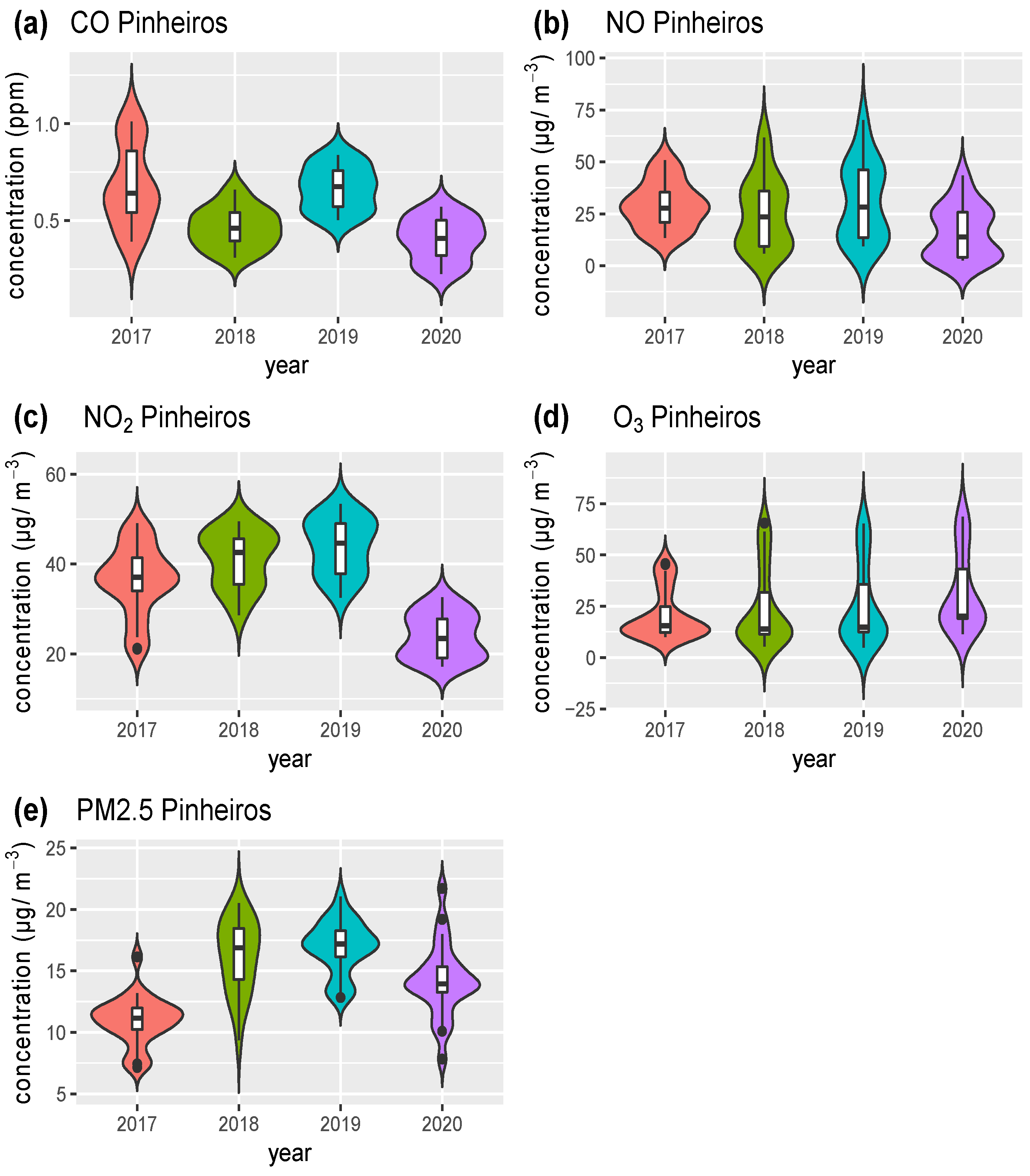
Figure 16 displays the violin graphs of the median of pollutants for the Pinheiros station. In Figure 16a–c for CO, NO and NO₂ the concentrations are lower in the year 2020, during the pandemic. This station is located close to Marginal Pinheiros, one of the main transit routes in the MASP, which is why there was a reduction in these pollutants. As it is a station close to the vehicular emission source, there is no significant variation in the secondary pollutant O₃ in the pandemic year. PM2.5 is lower in 2020 than in 2018 and 2019, but higher than in 2017.

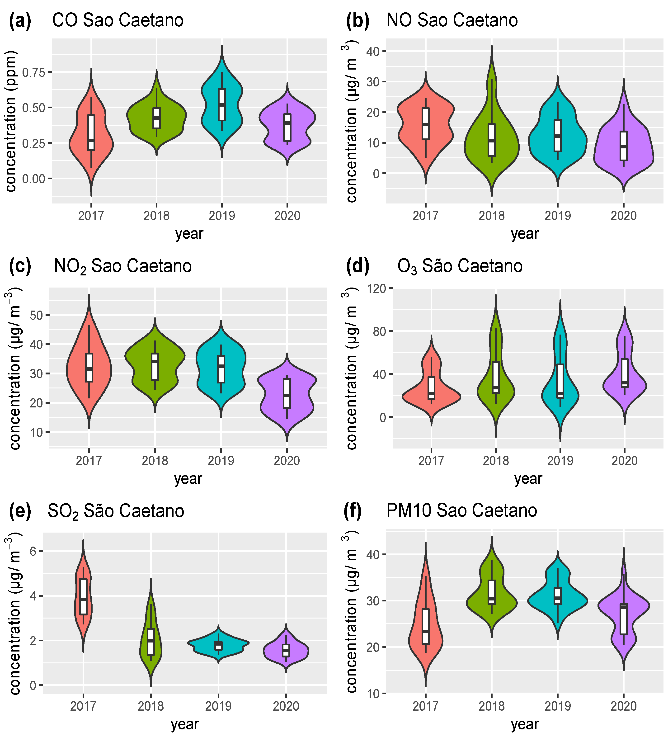
Figure 17 displays the violin graphs for São Caetano station. Figure 17a,b shows CO and NO, respectively. The year 2020 during the pandemic has the lowest median, but the data distribution is similar for all the years in this study (i.e., 2017–2020).

In Figure 17c, NO₂ has a lower median in 2020, during the pandemic, with reduced upper and lower limit values. Figure 17d shows O₃ with a higher median in 2020, during the pandemic, than in the pre-pandemic period, but with a similar data distribution. Figure 17e indicates the SO₂ with the lowest median in 2020, during the pandemic, but it is not very different from the 2019 value. Figure 17f for PM10 shows a lower median in 2020 (during the pandemic) than in 2018 and 2019 (during the pre-pandemic period). Overall, in the case of the MASP AQMS (Figure 12, Figure 13, Figure 14, Figure 15, Figure 16 and Figure 17), the violin graphs have a lower median concentration of CO, NO, and NO₂ for the pandemic period (April and May 2020) than for the pre-pandemic years (April and May 2017, 2018, and 2019), ozone has a higher median in the year of the pandemic owing to the reduction in NO that consumes O₃. CO, NO, NO₂, and O₃ have a similar distribution for the entire study period, while SO₂, PM10 and PM2.5 have a data distribution with a different pattern during the years 2017 to 2020.

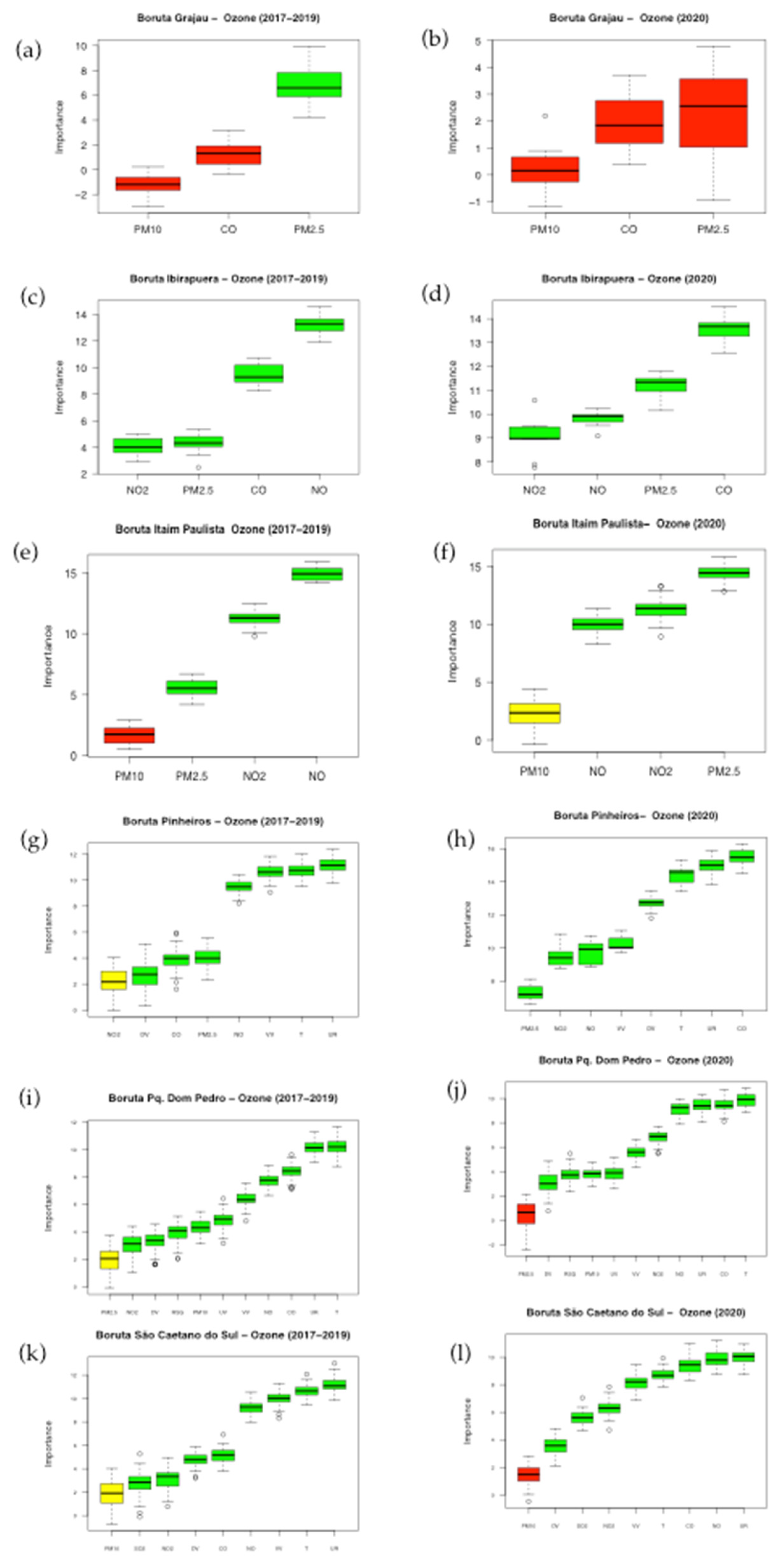
Figure 18a,b shows the importance of using the Boruta algorithm for pollutants with regard to tropospheric O₃, since Boruta is a well-tested resource selection method. It is designed to capture all the important and useful features you might have in your dataset with regard to an outcome variable. In this case, the study variable is the ozone concentration, and the dataset includes the other variables for the stations employed for monitoring air quality. In this study, green boxes are the most important variables for the formation or consumption of ozone, followed by the least important—yellow—and then red (medium and lower importance, respectively) [55].

In Figure 18a,b, the order does not change in the years during the pandemic and the pre-pandemic period, with PM2.5 and CO being the two pollutants in the Grajaú station that most influence O₃ formation. CO was the pollutant emitted in greatest abundance in the MASP, as shown in Figure 7, since it is partly oxidized to CO₂ by the hydroxyl radical, as outlined in Reaction 6, and it generates the hydroperoxide radical (HO₂). This radical, in a similar way to peroxide radicals, which are formed by VOCs, oxidizes NO to NO₂ by competing with O₃ molecules and increasing the atmospheric concentration of this gas, as outlined in Reaction 7.

CO + OH• → CO₂ + HO₂•

(6)

HO₂• + NO → NO₂ + OH•

(7)

Thus, the importance of this pollutant in the formation of O₃ can be explained both at the Grajaú station and at other stations that measure CO. At the Grajaú station, (Figure 18a,b), PM2.5 is the most important pollutant for O₃ formation in both periods, during and before the pandemic. In Figure 18c,d (Ibirapuera station), CO was the second most important pollutant for O₃ formation in the pre-pandemic period and the first pollutant in the pandemic year. At the Pinheiros station (Figure 18g,h), CO is the second most important pollutant in the pre-pandemic years and the first in the pandemic year. At the Parque Dom Pedro station (Figure 18i,j), CO is the first major pollutant in the pre-pandemic years and the second in the year during the pandemic. At the São Caetano do Sul station (Figure 18k,l), CO is the second most important pollutant for O₃ formation in both the pre-pandemic period and during the pandemic years.

Ref. [56] showed that an increase in atmospheric oxidation could strengthen the production of secondary particles by making a contribution of up to 27% to the environmental levels of PM2.5. High concentrations of O₃, a powerful oxidant, lead to the formation of secondary particles, which can result in O₃ being important in the formation of secondary particles. The interaction between O₃ and PM2.5 is generally affected by photochemical reactions [57]. Photolysis of O₃ generates OH·, which then oxidizes the VOCs to bring about the conversion of NO to NO₂, by breaking the photo-stationary state relationship. In addition to photochemical reactions, the heterogeneous reactions that occur on the surface of soluble particulate material and black carbon are also an important form of interaction between O₃ and atmospheric particles [58,59,60].

The authors of [61] analyzed data collected from diffuse reflectance infrared Fourier transform spectroscopy (DRIFTS) and reported that, in the presence of O₃, SO₂ could be oxidized to sulfate on the surface of CaCO₃ particles. The authors [62] found that high concentrations of NOx can largely increase the formation of fine particulate nitrate under high O₃ and in favorable meteorological conditions. Secondary organic and inorganic aerosols generated from oxidation reactions comprise a significant fraction of particles, which has serious implications for air pollution in large cities [63].

The authors of [64,65] used a box model and a three-dimensional regional chemical transport model to assess the impact of dust particles on tropospheric photochemistry over the megacity of Beijing with high concentrations of dust leveling down the O₃ environment [66] analyzed summer O₃ formation in a megacity in northwest China and concluded that high concentrations of particulate matter can significantly reduce the photolysis frequencies with O₃ reduced by more than 50 µg·m⁻³ (about 25 ppb).

High NOx concentrations can increase fine particulate nitrate formation at high O₃ levels depending on weather conditions [62,67]. At the Ibirapuera station, which is classified as a background station, since it is a long distance from the roads with the highest emissions of primary pollutants (Figure 18c,d), PM2.5 was the third most important pollutant for O₃ formation in the pre-pandemic period, and in the year during the pandemic as the second most important pollutant for O₃. At the residential/industrial Itaim Paulista station (Figure 18e,f), PM2.5 was the third most important pollutant for the formation of O₃ in the pre-pandemic period, and in the pandemic year, it was the first. At the Pinheiros and Parque Dom Pedro stations (Figure 18h–j), PM2.5 has no significant importance in O₃ formation. As these two stations (Pinheiros and Parque Dom Pedro) are close to the main roads in the MASP, with higher concentrations of primary pollutants such as CO and NO, there is no time for the formation of high O₃ concentrations and their interaction in the formation of fine and secondary particles, such as PM2.5. The background stations (Ibirapuera) and Itaim Paulista (residential/industrial), are far away from traffic routes with high emission rates of primary pollutants during the pandemic year, and thus PM2.5 has become more important in O₃ formation than NO. During the pandemic year, there was a decrease of 47.3% and 19.2% in NO at the stations of Ibirapuera and Itaim Paulista, respectively, with regard to the NO pollutant during the pandemic when compared with the pre-pandemic period. An increase of 27.3% in O₃ for the Ibirapuera station and 21.5% in O₃ at the Itaim Paulista station reduced the concentration of NO that consumes O₃ and increased the interaction of O₃ with the formation of PM2.5 particles.

At stations that measured NO (Ibirapuera, Itaim Paulista, Pinheiros, Parque Dom Pedro, and São Caetano do Sul), in the pre-pandemic period, NO was the most important for O₃ concentration. In this case, the consumption will later be formed of NO₂, which will undergo photolysis and form O₃ again (Figure 18c,e), and during the pandemic, this was the third most important pollutant (Figure 18d,f). At the Pinheiros station, NO is the first most important pollutant in the pre-pandemic period and the second most important pollutant during the pandemic year with regard to O₃ formation. At the Parque Dom Pedro station, NO was the second most important during the pre-pandemic period and the most important during the pandemic year. At the São Caetano do Sul station, NO was the most important in O₃ formation in both periods, i.e., during the pandemic and pre-pandemic. At Ibirapuera station, there was a reduction of 47.3% in NO concentrations, a reduction of 19.2% at Itaim Paulista, a reduction of 75.6% at Pinheiros, a 37% reduction at Parque Dom Pedro, and a 45.5% reduction at São Caetano do Sul during the pandemic, compared with the pre-pandemic period. The NO pollutant consumes O₃ to form NO₂ and the decrease in NO during the pandemic period had the effect of increasing the O concentration. This phenomenon was also observed in Rio de Janeiro and is examined in a study [68].

The AQMS São Caetano do Sul, classified as residential, and Ibirapuera, classified as urban background, showed the greatest reduction of PM2.5, 30.1, and 20.7%, respectively, since these two stations tend to have higher O₃ concentrations, because they are far from the main routes that emit primary pollutants. The greater decrease in PM2.5 in these two stations can probably be attributed to a higher concentration of O₃; perhaps NOx in these stations allows the formation of O₃ rather than PM2.5. The stations of Grajaú-Parelheiros, Itaim Paulista, and Parque Dom Pedro had an average variation in the hourly concentration of PM2.5 during the pandemic, which was practically insignificant compared with the pre-pandemic period. The Pinheiros station experienced an increase of 20.5% in its average hourly concentrations during the pandemic period. This station is close to one of the main vehicular traffic routes of MASP, and was the station that had the greatest reduction in NO and NO₂ and the second largest increase in O₃, despite being a station with a high concentration of primary pollutants. This increase in PM2.5 can probably be attributed to a higher concentration of O₃ in the formation of secondary organic particles, which led to an increase in the concentration of PM2.5.

In general, in Figure 16, Figure 17 and Figure 18 the pollutants NO₂, SO₂, and PM10 had less importance in the O₃ concentration than CO, NO, and PM2.5, which were the most serious pollutants for the O₃ levels.

The key meteorological variables for tropospheric O₃ concentration in the MASP in the three stations that measure these variables were relative humidity, temperature, and wind speed. As there were no significant changes in these parameters in the years during the pandemic and pre-pandemic periods, it is impossible to compare their variables. However, it can be inferred that a rise in temperature increases the concentration of O₃ as it has a linear relationship with solar radiation. Wind intensity can lead to air masses that carry O₃ precursors or themselves. Several studies have shown a positive Pearson correlation of O₃ with temperature and wind speed and a negative correlation with relative humidity in the MASP (cf. [69,70]. In another study, specifically concerned with O₃, [70] analyzed 39 large urban areas in the eastern US, which confirmed that O₃ generally increases when there is a rise in temperature and decreases when there is greater relative humidity.

4. Conclusions

Overall, this work made a diagnosis of reductions in pollutants that were experienced in the initial period of the COVID pandemic and lockdown in São Paulo State and three other states (Rio de Janeiro, Minas Gerais, and Espírito Santo), which comprise an area larger than 924.511 km² in southeast Brazil. Additionally, 6 ground-based stations were used in different parts of São Paulo city. Similar results have been obtained in the literature, but the following advances have been made for other places, and these can be enumerated as follows:

(1)

Unprecedented work throughout South America in terms of this special issue;

(2)

Analyses of different chemical components (CO, NO, SO₂, NO₂, NOx, O₃, BC, PM2.5, and aerosols);

(3)

A combination of several data sources from reanalysis, in situ data, and remote sensing; and

(4)

A successful study that explores the use of satellite data combined with ground-level observations.

With regard to this last topic, it is clear that although the remote sensing information creates different spatial and temporal resolutions and distinct conceptions from in situ observations (integrated atmospheric column inference versus surface measurements), these were able to point in the same direction, and thus become supplementary tools for the advancement of air quality studies and monitoring.

Data from the pollution map of the southeast region of Brazil of NO₂ (OMI) and CO, SO₂, and BC (MERRA-2) showed that the reduction in the concentration of the NO₂ pollutant for the period of the pandemic, compared with the period before the pandemic, ranged from 10% to more than 60% for the area of the MASP and MARJ region, and a decrease in NO₂ of around 10% in the MABH and MAV. The concentrations of CO and BC from MERRA-2 fell by around 10% during the lockdown period in almost the entire state of SP, particularly on the border between the states of SP and RJ. The concentrations of SO₂ from MERRA-2 were 5 to 10% lower in the area of MASP and MARJ and the west of the MABH, with a decrease of between 30% and 50% on the border between the states of SP and RJ. In the MAV, an increase in the SO₂ pollutant was observed, since during the period of this study, this area was not yet greatly affected by the COVID-19 pandemic.

With regard to the MASP air quality data from the monitoring stations, the results showed the impact of a partial lockdown on the air quality of the Metropolitan Area of São Paulo. The partially mandated social restrictions, reduction in road traffic, and reduced economic activity led to a decrease in CO, NO, and NO₂ levels and, in contrast, an increase in O₃ concentrations. Similar results were observed in 2018 during a 10-day truck driver’s strike that took place throughout Brazil. Primary pollutants directly linked to vehicle emissions, such as CO and NO, decreased dramatically in MASP in April and May 2020 during the partial lockdown. Statistically significant differences between periods during and before the pandemic were observed in almost all the stations analyzed for these pollutants. NO concentrations decreased by an average of 44.9%, and CO concentrations decreased (by 38.8%) during the partial lockdown period in 2020 compared with the pre-pandemic period. In the case of NO₂ the average reduction was 38.7%. Concerning PM2.5, there was a decrease at three stations, an average of 14% lower, and an increase of 20.5% at the Pinheiros station, 2.9% at the Itaim Paulista, and 4.6% at the Parque Dom Pedro station. This shows the complexity of this pollutant, which consists of several different sources, including many secondary reactions in the atmosphere. In the case of O₃, concentrations increased by an average of 16%. In theory, this increase in O₃ was due to a decrease in NOx, since in an NOx-saturated system such as in MASP, falling NOx concentrations lead to an increase in O₃, and decreasing VOC concentrations reduce the O₃.

According to Boruta graphs, the pollutants that most influence O₃ concentrations are CO, NO, and PM2.5, and in some AQMS, such as Ibirapuera and Itaim Paulista stations that are farther away from the main roads where there is heavier traffic. This means that in monitoring stations with lower primary pollutant concentrations and higher O₃ concentration, PM2.5 proved to be more important in the O₃ concentration than NO during the pandemic period, since there was a significant decrease in NO in these stations and probably a greater interaction of O₃ with particulate matter leading to the formation of PM2.5. In addition to photochemical reactions, the heterogeneous reactions that occur on the surface of particulate matter are also an important means for interaction between O₃ and atmospheric particles.

This work can be replicated in other cities in the northern hemisphere, such as South Asia and North America, where several articles similar to this have been published using satellite, modeling, and monitoring station data to compare the period of the lockdown caused by the COVID-19 virus and the preceding period without a pandemic [26,28,71].

These results show that MASP pollution is influenced to a great extent by vehicular emissions. Clearly, improvements in controlling vehicle emissions directly from vehicle exhausts, maintenance, and the quality of all types of fuels are necessary to reduce primary emissions, and the implementation of better measures to enhance urban mobility and public transport would greatly benefit the urban environment and the health of the inhabitants of the MASP.

References

1. CETESB. Air Quality Report for the Sao Paulo State 2019; Environmental Agency of the State of São Paulo: São Paulo, Brazil, 2020. [Google Scholar]
2. World Health Organization. WHO Director-General’s Opening Remarks at the Media Briefing on COVID-19—11 March 2020; World Health Organization: Geneva, Switzerland, 2020. [Google Scholar]
3. Brasil Ministry of Health. COVID19—Coronavirus Panel 2022; Brasil Ministry of Health: Rio de Janeiro, Brasil, 2022. [Google Scholar]
4. SEADE. Covid; Seade, State Data Analysis System Foundation: Sao Paulo, Brazil, 2022. [Google Scholar]
5. Croda, J.; de Oliveira, W.K.; Frutuoso, R.L.; Mandetta, L.H.; Baia-da-Silva, D.C.; Brito-Sousa, J.D.; Monteiro, W.M.; Lacerda, M.V.G. COVID-19 in Brazil: Advantages of a Socialized Unified Health System and Preparation to Contain Cases. Rev. Soc. Bras. Med. Trop. 2020, 53, e20200167. [Google Scholar] [CrossRef] [PubMed]
6. São Paulo State. Decree n. 64,881, of March 22, 2020. 2020. Available online: https://www.al.sp.gov.br/repositorio/legislacao/decreto/2020/decreto-64881-22.03.2020.html (accessed on 1 October 2022).
7. Wang, H.; Naghavi, M.; Allen, C.; Barber, R.M.; Bhutta, Z.A.; Carter, A.; Casey, D.C.; Charlson, F.J.; Chen, A.Z.; Coates, M.M.; et al. Global, Regional, and National Life Expectancy, All-Cause Mortality, and Cause-Specific Mortality for 249 Causes of Death, 1980–2015: A Systematic Analysis for the Global Burden of Disease Study 2015. Lancet 2016, 388, 1459–1544. [Google Scholar] [CrossRef] [PubMed] [Green Version]
8. Forster, P.M.F.; Taylor, K.E. Climate Forcings and Climate Sensitivities Diagnosed from Coupled Climate Model Integrations. J. Clim. 2006, 19, 6181–6194. [Google Scholar] [CrossRef]
9. Jacob, D.J.; Winner, D.A. Effect of Climate Change on Air Quality. Atmos. Environ. 2009, 43, 51–63. [Google Scholar] [CrossRef] [Green Version]
10. Duncan, B.N.; Prados, A.I.; Lamsal, L.N.; Liu, Y.; Streets, D.G.; Gupta, P.; Hilsenrath, E.; Kahn, R.A.; Nielsen, J.E.; Beyersdorf, A.J.; et al. Satellite Data of Atmospheric Pollution for U.S. Air Quality Applications: Examples of Applications, Summary of Data End-User Resources, Answers to FAQs, and Common Mistakes to Avoid. Atmos. Environ. 2014, 94, 647–662. [Google Scholar] [CrossRef] [Green Version]
11. Deeter, M.N.; Edwards, D.P.; Gille, J.C.; Worden, H.M. Information Content of MOPITT CO Profile Retrievals: Temporal and Geographical Variability: MOPITT Information Content Variability. J. Geophys. Res. Atmos. 2015, 120, 12723–12738. [Google Scholar] [CrossRef]
12. Drummond, J.R.; Zou, J.; Nichitiu, F.; Kar, J.; Deschambaut, R.; Hackett, J. A Review of 9-Year Performance and Operation of the MOPITT Instrument. Adv. Space Res. 2010, 45, 760–774. [Google Scholar] [CrossRef]
13. Deeter, M.N.; Martínez-Alonso, S.; Gatti, L.V.; Gloor, M.; Miller, J.B.; Domingues, L.G.; Correia, C.S.C. Validation and Analysis of MOPITT CO Observations of the Amazon Basin. Atmos. Meas. Tech. 2016, 9, 3999–4012. [Google Scholar] [CrossRef] [Green Version]
14. Kaufman, Y.J.; Tanré, D.; Boucher, O. A Satellite View of Aerosols in the Climate System. Nature 2002, 419, 215–223. [Google Scholar] [CrossRef]
15. Alvim, D.S.; Chiquetto, J.B.; D’Amelio, M.T.S.; Khalid, B.; Herdies, D.L.; Pendharkar, J.; Corrêa, S.M.; Figueroa, S.N.; Frassoni, A.; Capistrano, V.B.; et al. Evaluating Carbon Monoxide and Aerosol Optical Depth Simulations from CAM-Chem Using Satellite Observations. Remote Sens. 2021, 13, 2231. [Google Scholar] [CrossRef]
16. Cooper, M.J.; Martin, R.V.; Hammer, M.S.; Levelt, P.F.; Veefkind, P.; Lamsal, L.N.; Krotkov, N.A.; Brook, J.R.; McLinden, C.A. Global Fine-Scale Changes in Ambient NO2 during COVID-19 Lockdowns. Nature 2022, 601, 380–387. [Google Scholar] [CrossRef]
17. Buchwitz, M.; Reuter, M.; Schneising, O.; Noël, S.; Gier, B.; Bovensmann, H.; Burrows, J.P.; Boesch, H.; Anand, J.; Parker, R.J.; et al. Computation and Analysis of Atmospheric Carbon Dioxide Annual Mean Growth Rates from Satellite Observations during 2003–2016. Atmos. Chem. Phys. 2018, 18, 17355–17370. [Google Scholar] [CrossRef] [Green Version]
18. Cadotte, M. Early Evidence That COVID-19 Government Policies Reduce Urban Air Pollution; National Library of Medicine: Bethesda, MD, USA, 2020. [Google Scholar]
19. Nakada, L.Y.K.; Urban, R.C. COVID-19 Pandemic: Impacts on the Air Quality during the Partial Lockdown in São Paulo State, Brazil. Sci. Total Environ. 2020, 730, 139087. [Google Scholar] [CrossRef]
20. Alvim, D.S.; Chiquetto, J.B.; Rozante, J.R.; Herdies, D.L.; Conti, L.M.; Rozante, V.; Gobo, J.P.A.; Faria, M.; dos Santos, A.F.; Figueroa, S.N. Truck Drivers’ Strike and the decrease of pollutants carbon monoxide and nitrogen oxides and the increase of ozone in the metropolitan area of São Paulo. In Geosciences: Establishment and Evolution of Human Civilization 2; Pergamon: Athens, Greece, 2020; pp. 35–53. ISBN 9786557065556. [Google Scholar]
21. Chiquetto, J.B.; Alvim, D.S.; Rozante, J.R.; Faria, M.; Rozante, V.; Gobo, J.P.A. Impact of a Truck Driver’s Strike on Air Pollution Levels in São Paulo. Atmos. Environ. 2020, 246, 118072. [Google Scholar] [CrossRef]
22. Ahmed, M.M.; Hoque, M.d.E.; Rahman, S.; Roy, P.K.; Alam, F.; Rahman, M.M.; Rahman, M.d.M.; Hopke, P.K. Prediction of COVID-19 Cases from the Nexus of Air Quality and Meteorological Phenomena: Bangladesh Perspective. Earth Syst. Environ. 2022, 6, 307–325. [Google Scholar] [CrossRef]
23. Zambrano-Monserrate, M.A.; Ruano, M.A.; Sanchez-Alcalde, L. Indirect Effects of COVID-19 on the Environment. Sci. Total Environ. 2020, 728, 138813. [Google Scholar] [CrossRef]
24. Tobías, A.; Carnerero, C.; Reche, C.; Massagué, J.; Via, M.; Minguillón, M.C.; Alastuey, A.; Querol, X. Changes in Air Quality during the Lockdown in Barcelona (Spain) One Month into the SARS-CoV-2 Epidemic. Sci. Total Environ. 2020, 726, 138540. [Google Scholar] [CrossRef]
25. Sharma, S.; Zhang, M.; Gao, J.; Zhang, H.; Kota, S.H. Effect of Restricted Emissions during COVID-19 on Air Quality in India. Sci. Total Environ. 2020, 728, 138878. [Google Scholar] [CrossRef]
26. Hu, Z.; Jin, Q.; Ma, Y.; Ji, Z.; Zhu, X.; Dong, W. How Does COVID-19 Lockdown Impact Air Quality in India? Remote Sens. 2022, 14, 1869. [Google Scholar] [CrossRef]
27. Grzybowski, P.T.; Markowicz, K.M.; Musiał, J.P. Reduction of Air Pollution in Poland in Spring 2020 during the Lockdown Caused by the COVID-19 Pandemic. Remote Sens. 2021, 13, 3784. [Google Scholar] [CrossRef]
28. Ghahremanloo, M.; Lops, Y.; Choi, Y.; Mousavinezhad, S. Impact of the COVID-19 Outbreak on Air Pollution Levels in East Asia. Sci. Total Environ. 2021, 754, 142226. [Google Scholar] [CrossRef]
29. Zhao, X.; Fioletov, V.; Alwarda, R.; Su, Y.; Griffin, D.; Weaver, D.; Strong, K.; Cede, A.; Hanisco, T.; Tiefengraber, M.; et al. Tropospheric and Surface Nitrogen Dioxide Changes in the Greater Toronto Area during the First Two Years of the COVID-19 Pandemic. Remote Sens. 2022, 14, 1625. [Google Scholar] [CrossRef]
30. Anand, V.; Korhale, N.; Tikle, S.; Rawat, M.S.; Beig, G. Is Meteorology a Factor to COVID-19 Spread in a Tropical Climate? Earth Syst. Environ. 2021, 5, 939–948. [Google Scholar] [CrossRef] [PubMed]
31. IBGE. 2021 Brazilian Census; Brazilian Institute of Geography and Statistics: Rio de Janeiro, Brazil, 2022. [Google Scholar]
32. de Lima, G.N.; Magaña Rueda, V.O. The Urban Growth of the Metropolitan Area of Sao Paulo and Its Impact on the Climate. Weather Clim. Extrem. 2018, 21, 17–26. [Google Scholar] [CrossRef]
33. Vemado, F.; Pereira Filho, A.J. Severe Weather Caused by Heat Island and Sea Breeze Effects in the Metropolitan Area of São Paulo, Brazil. Adv. Meteorol. 2016, 2016, 1–13. [Google Scholar] [CrossRef] [Green Version]
34. Bahl, R.W.; Linn, J.F.; Wetzel, D.L. (Eds.) Financing Metropolitan Governments in Developing Countries; Lincoln Institute of Land Policy: Cambridge, MA, USA, 2013; ISBN 978-1-55844-254-2. [Google Scholar]
35. Leirião, L.F.L.; Miraglia, S.G.E.K. Environmental and Health Impacts Due to the Violation of Brazilian Emissions Control Program Standards in Sao Paulo Metropolitan Area. Transp. Res. Part Transp. Environ. 2019, 70, 70–76. [Google Scholar] [CrossRef]
36. Levelt, P.F.; van den Oord, G.H.J.; Dobber, M.R.; Malkki, A.; Visser, H.; de Vries, J.; Stammes, P.; Lundell, J.O.V.; Saari, H. The Ozone Monitoring Instrument. IEEE Trans. Geosci. Remote Sens. 2006, 44, 1093–1101. [Google Scholar] [CrossRef]
37. Kalnay, E. Atmospheric Modeling, Data Assimilation and Predictability, 1st ed.; Cambridge University Press: Cambridge, UK, 2002; ISBN 978-0-521-79179-3. [Google Scholar]
38. Rienecker, M.M.; Suarez, M.J.; Gelaro, R.; Todling, R.; Bacmeister, J.; Liu, E.; Bosilovich, M.G.; Schubert, S.D.; Takacs, L.; Kim, G.-K.; et al. MERRA: NASA’s Modern-Era Retrospective Analysis for Research and Applications. J. Clim. 2011, 24, 3624–3648. [Google Scholar] [CrossRef]
39. WHO (Ed.) Air Quality Guidelines for Europe, WHO regional publications European series, 2nd ed.; World Health Organization, Regional Office for Europe: Copenhagen, Denmark, 2000; ISBN 978-92-890-1358-1. [Google Scholar]
40. Breuer, D. (Ed.) Monitoring Ambient Air Quality for Health Impact Assessment; WHO regional publications; World Health Organization, Regional Office for Europe: Copenhagen, Denmark, 1999; ISBN 978-92-890-1351-2. [Google Scholar]
41. Martin, F.; Fileni, L.; Palomino, I.; Vivanco, M.G.; Garrido, J.L. Analysis of the Spatial Representativeness of Rural Background Monitoring Stations in Spain. Atmos. Pollut. Res. 2014, 5, 779–788. [Google Scholar] [CrossRef] [Green Version]
42. Randles, C.A.; da Silva, A.M.; Buchard, V.; Colarco, P.R.; Darmenov, A.; Govindaraju, R.; Smirnov, A.; Holben, B.; Ferrare, R.; Hair, J.; et al. The MERRA-2 Aerosol Reanalysis, 1980 Onward. Part I: System Description and Data Assimilation Evaluation. J. Clim. 2017, 30, 6823–6850. [Google Scholar] [CrossRef]
43. Buchard, V.; Randles, C.A.; da Silva, A.M.; Darmenov, A.; Colarco, P.R.; Govindaraju, R.; Ferrare, R.; Hair, J.; Beyersdorf, A.J.; Ziemba, L.D.; et al. The MERRA-2 Aerosol Reanalysis, 1980 Onward. Part II: Evaluation and Case Studies. J. Clim. 2017, 30, 6851–6872. [Google Scholar] [CrossRef]
44. Holben, B.N.; Tanré, D.; Smirnov, A.; Eck, T.F.; Slutsker, I.; Abuhassan, N.; Newcomb, W.W.; Schafer, J.S.; Chatenet, B.; Lavenu, F.; et al. An Emerging Ground-Based Aerosol Climatology: Aerosol Optical Depth from AERONET. J. Geophys. Res. Atmos. 2001, 106, 12067–12097. [Google Scholar] [CrossRef]
45. Dantas, G.; Siciliano, B.; França, B.B.; da Silva, C.M.; Arbilla, G. The Impact of COVID-19 Partial Lockdown on the Air Quality of the City of Rio de Janeiro, Brazil. Sci. Total Environ. 2020, 729, 139085. [Google Scholar] [CrossRef]
46. CETESB. Air Quality Report for the Sao Paulo State 2021; Environmental Agency of the State of São Paulo: São Paulo, Brazil, 2021. [Google Scholar]
47. Chiquetto, J.B.; Silva, M.E.S.; Ynoue, R.Y.; Dutra Ribieiro, F.N.; Alvim, D.S.; Rozante, J.R.; Cabral-Miranda, W.; Swap, R.J. The impact of different urban land use types on air pollution in the megacity of São Paulo. Rev. Presença Geográfica 2020, 7, 91. [Google Scholar] [CrossRef]
48. Orlando, J.P.; Alvim, D.S.; Yamazaki, A.; Corrêa, S.M.; Gatti, L.V. Ozone Precursors for the São Paulo Metropolitan Area. Sci. Total Environ. 2010, 408, 1612–1620. [Google Scholar] [CrossRef]
49. Alvim, D.S.; Gatti, L.V.; Corrêa, S.M.; Chiquetto, J.B.; de Souza Rossatti, C.; Pretto, A.; dos Santos, M.H.; Yamazaki, A.; Orlando, J.P.; Santos, G.M. Main Ozone-Forming VOCs in the City of Sao Paulo: Observations, Modelling and Impacts. Air Qual. Atmos. Health 2017, 10, 421–435. [Google Scholar] [CrossRef]
50. Alvim, D.S.; Gatti, L.V.; Corrêa, S.M.; Chiquetto, J.B.; Santos, G.M.; de Souza Rossatti, C.; Pretto, A.; Rozante, J.R.; Figueroa, S.N.; Pendharkar, J.; et al. Determining VOCs Reactivity for Ozone Forming Potential in the Megacity of São Paulo. Aerosol Air Qual. Res. 2018, 18, 2460–2474. [Google Scholar] [CrossRef]
51. Alvim, D.S.; Gatti, L.V.; Corrêa, S.M.; Chiquetto, J.B.; Pendharkar, J.; Pretto, A.; Santos, G.M.; Rossati, C.D.S.; Herdies, D.L.; Figueroa, S.N.; et al. Concentrations of Volatile Organic Compounds in the Megacity of São Paulo in 2006 and 2011/2012—A Comparative Study. Anuário Inst. Geociências 2020, 43. [Google Scholar] [CrossRef]
52. Wang, H.; Huang, C.; Tao, W.; Gao, Y.; Wang, S.; Jing, S.; Wang, W.; Yan, R.; Wang, Q.; An, J.; et al. Seasonality and Reduced Nitric Oxide Titration Dominated Ozone Increase during COVID-19 Lockdown in Eastern China. Npj Clim. Atmos. Sci. 2022, 5, 24. [Google Scholar] [CrossRef]
53. Benton, A.K.; Langridge, J.M.; Ball, S.M.; Bloss, W.J.; Dall’Osto, M.; Nemitz, E.; Harrison, R.M.; Jones, R.L. Night-Time Chemistry above London: Measurements of NO3 and N2O5 from the BT Tower. Atmos. Chem. Phys. 2010, 10, 9781–9795. [Google Scholar] [CrossRef] [Green Version]
54. Lin, C.; Hu, R.; Xie, P.; Lou, S.; Zhang, G.; Tong, J.; Liu, J.; Liu, W. Nocturnal Atmospheric Chemistry of NO3 and N2O5 over Changzhou in the Yangtze River Delta in China. J. Environ. Sci. 2022, 114, 376–390. [Google Scholar] [CrossRef] [PubMed]
55. Kursa, M.B.; Rudnicki, W.R. Feature Selection with the Boruta Package. J. Stat. Softw. 2010, 36, 1–13. [Google Scholar] [CrossRef] [Green Version]
56. Jia, M.; Zhao, T.; Cheng, X.; Gong, S.; Zhang, X.; Tang, L.; Liu, D.; Wu, X.; Wang, L.; Chen, Y. Inverse Relations of PM2.5 and O3 in Air Compound Pollution between Cold and Hot Seasons over an Urban Area of East China. Atmosphere 2017, 8, 59. [Google Scholar] [CrossRef] [Green Version]
57. Meng, Z.; Dabdub, D.; Seinfeld, J.H. Chemical Coupling Between Atmospheric Ozone and Particulate Matter. Science 1997, 277, 116–119. [Google Scholar] [CrossRef] [Green Version]
58. Ravishankara, A.R. Heterogeneous and Multiphase Chemistry in the Troposphere. Science 1997, 276, 1058–1065. [Google Scholar] [CrossRef]
59. Li, G.; Zhang, R.; Fan, J.; Tie, X. Impacts of Black Carbon Aerosol on Photolysis and Ozone. J. Geophys. Res. 2005, 110, D23206. [Google Scholar] [CrossRef] [Green Version]
60. Li, J.; Wang, Z.; Wang, X.; Yamaji, K.; Takigawa, M.; Kanaya, Y.; Pochanart, P.; Liu, Y.; Irie, H.; Hu, B.; et al. Impacts of Aerosols on Summertime Tropospheric Photolysis Frequencies and Photochemistry over Central Eastern China. Atmos. Environ. 2011, 45, 1817–1829. [Google Scholar] [CrossRef]
61. Li, L.; Chen, Z.M.; Zhang, Y.H.; Zhu, T.; Li, J.L.; Ding, J. Kinetics and Mechanism of Heterogeneous Oxidation of Sulfur Dioxide by Ozone on Surface of Calcium Carbonate. Atmos. Chem. Phys. 2006, 6, 2453–2464. [Google Scholar] [CrossRef] [Green Version]
62. Ge, B.; Sun, Y.; Liu, Y.; Dong, H.; Ji, D.; Jiang, Q.; Li, J.; Wang, Z. Nitrogen Dioxide Measurement by Cavity Attenuated Phase Shift Spectroscopy (CAPS) and Implications in Ozone Production Efficiency and Nitrate Formation in Beijing, China: NITROGEN DIOXIDE MEASUREMENT BY CAPS. J. Geophys. Res. Atmos. 2013, 118, 9499–9509. [Google Scholar] [CrossRef]
63. Huang, R.-J.; Zhang, Y.; Bozzetti, C.; Ho, K.-F.; Cao, J.-J.; Han, Y.; Daellenbach, K.R.; Slowik, J.G.; Platt, S.M.; Canonaco, F.; et al. High Secondary Aerosol Contribution to Particulate Pollution during Haze Events in China. Nature 2014, 514, 218–222. [Google Scholar] [CrossRef] [Green Version]
64. Zhu, S.; Butler, T.; Sander, R.; Ma, J.; Lawrence, M.G. Impact of Dust on Tropospheric Chemistry over Polluted Regions: A Case Study of the Beijing Megacity. Atmos. Chem. Phys. 2010, 10, 3855–3873. [Google Scholar] [CrossRef] [Green Version]
65. Xu, J.; Zhang, Y.; Wang, W. Numerical Study on the Impacts of Heterogeneous Reactions on Ozone Formation in the Beijing Urban Area. Adv. Atmos. Sci. 2006, 23, 605–614. [Google Scholar] [CrossRef]
66. Feng, T.; Bei, N.; Huang, R.; Cao, J.; Zhang, Q.; Zhou, W.; Tie, X.; Liu, S.; Zhang, T.; Su, X.; et al. Summertime ozone formation in Xi’an and surrounding areas, China. Atmos. Chem. Phys. 2015, 15. [Google Scholar] [CrossRef] [Green Version]
67. Wen, L.; Xue, L.; Wang, X.; Xu, C.; Chen, T.; Yang, L.; Wang, T.; Zhang, Q.; Wang, W. Summertime Fine Particulate Nitrate Pollution in the North China Plain: Increasing Trends, Formation Mechanisms and Implications for Control Policy. Atmospheric Chem. Phys. 2018, 18, 11261–11275. [Google Scholar] [CrossRef] [Green Version]
68. Martins, E.M.; Nunes, A.C.L.; Corrêa, S.M. Understanding Ozone Concentrations During Weekdays and Weekends in the Urban Area of the City of Rio de Janeiro. J. Braz. Chem. Soc. 2015, 26, 1967–1975. [Google Scholar] [CrossRef]
69. Guardani, R.; Aguiar, J.L.; Nascimento, C.A.O.; Lacava, C.I.V.; Yanagi, Y. Ground-Level Ozone Mapping in Large Urban Areas Using Multivariate Statistical Analysis: Application to the São Paulo Metropolitan Area. J. Air Waste Manag. Assoc. 2003, 53, 553–559. [Google Scholar] [CrossRef] [Green Version]
70. Camalier, L.; Cox, W.; Dolwick, P. The Effects of Meteorology on Ozone in Urban Areas and Their Use in Assessing Ozone Trends. Atmos. Environ. 2007, 41, 7127–7137. [Google Scholar] [CrossRef]
71. Fardani, I.; Aji, R.R. Analysis of Changes in Air Quality in Major Cities Indonesia During COVID 19 Using Remote Sensing Data. IOP Conf. Ser. Earth Environ. Sci. 2021, 830, 012085. [Google Scholar] [CrossRef]
Figure 1. Location of the Metropolitan Area of São Paulo (MASP) in Brazil and its urban sprawl.
Remotesensing 15 01262 g001
Figure 2. Location of the six automated AQMS of this stud y: (a) Grajaú, (b) Ibirapuera Park, (c) Itaim Paulista, (d) Parque Dom Pedro, (e) Pinheiros, and (f) São Caetano do Sul. The monitoring points are indicated by yellow circles.
Remotesensing 15 01262 g002
Figure 3. NO2 atmospheric concentration near the surface for the period of April and May during the pandemic (2020) and pre-pandemic (2017–2019) periods from the OMI sensor, and the percentage differences between the pandemic and pre-pandemic periods.
Remotesensing 15 01262 g003
Figure 4. CO atmospheric concentrations near the surface for the period of April and May during the pandemic (2020) and pre-pandemic (2017–2019) from MERRA–2, and the percentage differences during the pandemic and pre-pandemic periods.
Remotesensing 15 01262 g004
Figure 5. SO2 concentration near the surface for the period of April and May during the pandemic (2020) and pre-pandemic (2017–2019) from MERRA–2, and the percentage differences during the pandemic and pre-pandemic periods.
Remotesensing 15 01262 g005
Figure 6. Concentration near the surface of BC for the period of April and May during the pandemic (2020) and pre-pandemic (2017–2019) from MERRA–2, and the percentage differences during the pandemic and pre-pandemic periods.
Remotesensing 15 01262 g006
Figure 7. CO hourly concentrations for MASP during April-May 2017–2019 (pre-pandemic) and 2020 (during the pandemic) from ground-level AQMS.
Remotesensing 15 01262 g007
Figure 8. NO hourly concentration for MASP during April-May 2017–2019 (pre-pandemic) and 2020 (during the pandemic).
Remotesensing 15 01262 g008
Figure 9. NO2 hourly concentration for MASP during April-May 2017–2019 (pre-pandemic) and 2020 (during the pandemic) from ground-level AQMS.
Remotesensing 15 01262 g009
Figure 10. O3 hourly concentration for MASP during April-May 2017–2019 (pre-pandemic) and 2020 (during the pandemic) from ground-level AQMS.
Remotesensing 15 01262 g010
Figure 11. PM2.5 hourly concentration for MASP during April-May 2017–2019 (pre-pandemic) and 2020 (during the pandemic) from ground-level AQMS.
Remotesensing 15 01262 g011
Figure 12. Violin graphs for Grajaú station during April to May 2017 to 2020 from ground AQMS.
Remotesensing 15 01262 g012
Figure 13. Violin graphs for Ibirapuera station during April to May 2017 to 2020 from ground AQMS.
Remotesensing 15 01262 g013
Figure 14. Violin graphs for Itaim Paulista station during April to May of 2017 to 2020 from ground AQMS.
Remotesensing 15 01262 g014
Figure 15. Violin graphs for Parque Dom Pedro station during April to May of 2017 to 2020 from ground AQMS.
Remotesensing 15 01262 g015
Figure 16. Violin graphs for Pinheiros station during April to May of 2017 to 2020 from ground AQMS.
Remotesensing 15 01262 g016
Figure 17. Violin graphs for São Caetano do Sul station during April to May of 2017 to 2020 from ground AQMS.
Remotesensing 15 01262 g017
Figure 18. The Boruta calculation pollutants and meteorological variables that are most important for O3 concentration (decrease or increase) in the MASP during the pandemic and pre-pandemic periods from ground AQMS.
Remotesensing 15 01262 g018