Abstract
Australian inland riparian wetlands located east of the Great Dividing Range exhibit unique, hydroecological characteristics. These flood-dependent aquatic systems located in water-limited regions are declining rapidly due to the competitive demand for water for human activities, as well as climate change and variability. However, there exist very few reliable data to characterize inundation change conditions and quantify the impacts of the loss and deterioration of wetlands. A long-term time record of wetland inundation maps can provide a crucial baseline to monitor, assess, and assist the management and conservation of wetland ecosystems. This study presents a random forest-based multi-index classification algorithm (RaFMIC) on the Google Earth Engine (GEE) platform to efficiently construct a temporally dense, three-decadal time record of inundation maps of the southeast Australian riparian inland wetlands. The method was tested over the Macquarie Marshes located in the semiarid region of NSW, Australia. The results showed a good accuracy when compared against high-spatial resolution imagery. The total inundated area was consistent with precipitation and streamflow patterns, and the temporal dynamics of vegetation showed good agreement with the inundation maps. The inundation time record was analysed to generate inundation probability maps, which were in a good agreement with frequently flooded areas simulated by a hydrodynamic model and the distribution of flood-dependent vegetation species. The long-term, time-dense inundation maps derived from the RaFMIC method can provide key information to assess the condition and health of wetland ecosystems and have the potential to improve wetland inventory with spatially explicit water regime information. RaFMIC can be adapted over other dryland wetlands, as an effective semiautomated method of mapping long-term inundation dynamics.
1. Introduction
Wetlands are important features of the natural landscape that provide numerous environmental benefits. Knowledge about the inundation and ecohydrological change dynamics of wetlands is important for their conservation and management. Among thousands of wetlands in Australia, 66 sites (extending over 8.3 million hectares) have been identified as ‘wetlands of international importance’ under the Ramsar Convention and ~900 have been labelled ‘nationally important wetlands’ [1,2,3]. The inland riparian wetlands in semiarid and arid regions located to the west of the Great Dividing Range of Australia exhibit unique hydrological and ecological characteristics. Generally, these inland wetlands are formed by rivers, which form braided channel systems over very large, flat floodplains. Depressions over these large floodplains are periodically inundated by natural flows and precipitation. These flood events drive multiple ecohydrological functions over the wetlands, such as: the breeding events of waterbirds, fish, and frogs; reducing flood impacts; recharging groundwater; improving water quality by absorbing pollutants; and carbon sequestration [4,5,6]. Natural flows into inland wetlands have been highly regulated to secure water for agricultural production, domestic water uses, and other needs. Regulated flows, climate change, and variability have directly affected the periodic inundation events, resulting in a rapid degradation of wetland vegetation and other flow-dependent freshwater ecosystems such as waterbird, amphibian, turtle, and fish habitats [7,8,9]. However, there exists little baseline underpinning to inform critical locations with frequent inundation, inundation change status, and associated ecological impacts on dryland inland wetlands with required spatial detail. A time-series of inundation maps can serve as a critical tool for rapid assessment and targeting for protection and for quantifying the impacts of water management and climate change on this critical ecosystem.
Satellite remote sensing offers a viable means to monitor inundation over a large spatial extent through time. The potential of mapping surface water bodies using optical sensors such as Landsat satellites has been explored over the last several decades [10,11,12] at the local floodplain [13], subcontinental/regional [14,15,16], continental [17], and global scales [18,19]. The optical remote sensing approach relies on the ability of water to largely absorb electromagnetic energy (hence, very little reflectance), especially at the longer wavelengths such as the near-infrared (NIR) and short-wave infrared (SWIR) ranges [11,20]. Some researchers have employed multiple spectral indices such as the Normalised Difference Vegetation Index (NDVI) [21] and Normalised Difference Water Index (NDWI), [22,23,24] integrated with classification techniques and decision trees, to map open water bodies [25,26], considering different water constituents and relate spectral characteristics. Applying topographic metrics-based mapping methods (e.g., [27,28,29]) further refined the mapping of the boundaries of surface water bodies.
Recently, Australia made significant progress to develop systematic and consistent surface water information, in order to assist water planning and disaster management such as fires, floods, droughts, etc. [17,30] The time-series dataset, “Water Observation from Space” (WOfS), later renamed as Digital Earth Australia (DEA) Water Observations (WO), was produced by Geoscience Australia by using the multidecadal archive of Landsat imagery over the Australian continent (https://www.dea.ga.gov.au/products/dea-water-observations, accessed on 10 July 2020). Then, the DEA Waterbodies (DEA-B) was followed to map the locations and the boundaries of more than 300,000 surface waterbodies (including dams, lakes, or large rivers) from the DEA-WO (https://www.dea.ga.gov.au/products/dea-waterbodies, accessed on 10 July 2020). The DEA-B dataset provides a summary of the temporal change of the surface water area within the polygon, offering new insights into water availability at important landscapes such as dams, lakes, etc., at the local scale. However, it showed inherent limitations in locating waterbodies with mixed vegetation [30], as the mapping method of DEA-WO was developed to identify wet pixels based on the spectral signature of water using the decision tree method. For example, it significantly underestimated surface water within vegetated wetlands, such as the Macquarie Marshes, NSW [31]. Hence, DEA-WO could not show critical individual wetlands (i.e., depressional areas with frequent inundation) making up the entire Marshes network. Similarly, the overall spatial representations of many other listed wetlands in the Australian wetlands database still remain crude.
Compared to mapping open waters, mapping wetlands and associated inundated areas is more challenging due to the complex physical environmental characteristics of wetlands. In wetlands, the viewing of standing water is limited by canopy cover, and observed spectral responses are strongly mixed with vegetation and soils [25,26,28,32,33]. Therefore, multiple spectral indices and bands, which are sensitive to vegetation, bare soils, and water, have been used in some of the previous studies to map wetland inundation by defining thresholds with decision trees (e.g., [13,33,34]). Such thresholds used in decision tree-based models, are determined by a training sample that provides a range of spectral responses representative of different water conditions [13]. These thresholds, however, are often time- and space- dependent (e.g., [35]); hence, adjustments are necessary for different images and classifications tailored for specific locations or particular dates [36,37]. Selecting thresholds over a time-series record can also be a subjective and complex process [33,38]. Therefore, developing a long-term time-record of inundation maps using such methods is extremely challenging and a time-consuming task. The recent SAR data-based wetland mapping methods [39,40,41] cannot be used to create a multidecadal historic data record of inundation maps due to the unavailability of said data.
To address these problems, the present study aims to develop a rapid and efficient method to generate a temporally dense, long-term time-record of wetland inundation maps using a Landsat data-based semiautomated approach. Further, this study explores the potential use of these inundation maps to identify ‘hot spots’ within the entire floodplain, i.e., key individual wetlands that make up the complex wetland network systems. These key individual wetlands are critical for ecosystem functioning and service, hence for decision support on environmental water releases. To achieve this, a random forest-based multi-index classification algorithm (RaFMIC) was employed to map wetland inundation change dynamics at a 30-m spatial resolution using the constellation of Landsat 5, 7, and 8 images. This was performed without using any predetermined thresholds or scene-to-scene pre- and post- inundation images, as required by some of the previous wetland mapping works. Unlike DEM-based methods, our method is independent of elevation data and associated limitations.
Multi-index classification (i.e., using multiple vegetation and water indices as input layers) allows to capture the complex vegetation and water response of wetlands effectively, compared to spectral band-based classification, while minimizing the effects of illumination conditions [33,42,43]. Machine learning methods have recently been employed by a number of researchers to map wetland inundation due to their robustness in capturing complex relationships between the datasets [44,45,46,47,48]. Here, the random forest works as a robust classification algorithm which is capable of capturing complex relationships between inputs (i.e., a range of spectral responses for the wet and dry surface areas) and outputs (i.e., wetland inundation), even with a small dataset [49]. The massive amount of imagery was analysed using the cloud-based geospatial data processing platform, the Google Earth Engine (GEE) [50]. GEE offers petabytes of a satellite imagery archive, ready-to-use spatial data products, and in-built functions, including machine learning algorithms such as the random forest. It is able to handle high volumes of long-term spatial datasets with high-speed parallel processing computational infrastructure using Google’s computational resources, and is flexible in modifications and testing [51]. The RaFMIC method on the GEE was tested over the Macquarie Marshes, a large inland riparian floodplain wetland located in a semiarid region of the northern part of the Murray-Darling River Basin in southeastern Australia. The long-term, time-dense inundation maps derived from remote sensing showed the potential to provide key information to assess the condition and health of wetland ecosystems due to climate change and human-induced impacts, and the potential to improve wetland inventory maps with spatially explicit water regime information.
2. Overview of the Methodology
The method used to map wetland inundation dynamics can be divided into three parts: multi-index data preparation, random forest classification, and validation. An overview of the methodology is given in Figure 1 and is elaborated upon in the following sections.
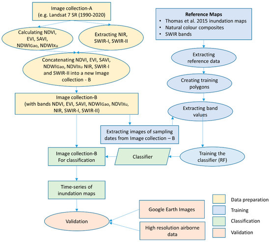
Figure 1.
Summary of the methodology followed in this study [13,21,22,23,24].
2.1. Multi-Index Approach Data Preparation
The Landsat SR image collections (named Image Collection-A in Figure 1) covering the study area were imported from the GEE data warehouse using an area filter for the extent of the study area and filtering off the images which had over a 10% cloud cover. Landsat images covering the extent of the study area were mosaicked by date to obtain the maximum coverage over the study area on each date. Afterwards, NDVI, Enhanced Vegetation Index (EVI), Soil Adjusted Vegetation Index (SAVI), NDWIGao, and NDVIXu were calculated, and NIR, SWIR-I, and SWIR-II bands were extracted from each Landsat image (refer to Annexure 1 for the band wavelengths of each Landsat mission). The indices and extracted bands were combined into mosaicked image collections on the GEE platform. These spectral bands and indices are capable of capturing various water and vegetation conditions and differentiating dryland from other land cover types; therefore, they conjointly have a good potential for describing wetland inundation characteristics of the Australian dryland inland wetlands [52,53,54]. The indices used in this study are briefly explained below.
The NDVI is the most widely used vegetation index in mapping vegetation. Chlorophyll in green vegetation absorbs solar radiation in blue (λ = 0.4–0.5 μm) and red (λ = 0.6–0.7 μm) ranges for photosynthesis, and the cell structure of leaves strongly reflects NIR (λ = 0.7 to 1.3 μm). NDVI is based on the difference between absorption and reflectance in the visible and NIR ranges of the electromagnetic spectrum on vegetation [21]. NDVI can be calculated as:
where NIR and RED are the spectral reflectance of the NIR and red ranges of the electromagnetic spectrum, respectively. NDVI values vary from −1 to 1. Generally, negative NDVI values represent water bodies, whereas values closer to 0 represent bare land and barren rocks. NDVI values ranging from 0.3 to 0.6 represent sparse vegetation, and higher NDVI values (>0.6) represent dense vegetation.
EVI is used to quantify vegetation greenness, similar to NDVI, but with some atmospheric corrections and adjustments for canopy background noise [55]. EVI is more sensitive to structural changes in canopies such as leaf area, compared to NDVI, which is more sensitive to chlorophyll content [56]. EVI is computed as:
where G is the gain factor, L is an adjustment for canopy background, C1 and C2 are coefficients for atmospheric resistance and B is the spectral reflectance of the blue range of the spectrum. For Landsat and Sentinel-2, G is 2.5, C1 is 6, C2 is 7.5, and L is 1 [57,58].
SAVI [59] is a modification of NDVI with a soil adjustment factor, L, to account for first-order soil–vegetation optical interactions and differential red and NIR extinction through the canopy. L = 0.5 is generally used to accommodate most vegetation types [60]. SAVI is computed as:
NDWI was first introduced by Gao [22], and later modified by McFeeters [23] and Xu [24], to distinguish water bodies from dryland. NDWIGao was focused on detecting vegetation water content by using NIR and SWIR bands. SWIR reflectance can account for vegetation water content and mesophyll structure in vegetation canopies, while NIR reflectance accounts for leaf internal structure and dry matter content, but not the water content. NDWIGao removed the changes induced by leaf internal structure and dry matter content, enhancing the vegetation water content. Since pure water reflects neither NIR nor SWIR, Xu [24] modified NDWI by replacing the NIR band with the green band (i.e., NDWIXu) and found an improvement in detecting floods, lakes, rivers, and seawater [61]. NDWIGao and NDWIXu are calculated as:
and
Apart from the above indices, NIR, SWIR-I, and SWIR-II bands of Landsat images were used in this study to map inundation dynamics. These bands are very sensitive to the presence of water, and effective in differentiating dry soils from other land cover types. The use of spectral indices can also minimise the effects of illumination differences of each day on the spectral bands, and between sensors. Accordingly, each image in a collection was converted into a multiband image consisting of the NDVI, EVI, SAVI, NDWIGao, and NDWIXu indices and the NIR, SWIR-I, and SWIR-II bands, and then combined as a new image collection (herein called image collection-B, as in Figure 1).
2.2. Image Classification
Training samples were carefully collected from the image collection-Bs (see Figure 1) on selected dates to capture a range of spectral responses from water, such as open surface water, and inundated areas with different types of vegetation in dryland inland wetlands. Here, training samples of three inundation classes, i.e., (i) open water, (ii) vegetation + water, and (iii) dryland, were collected from multiple images, separately, for each Landsat data collection (i.e., Landsat 5, 7, and 8). Existing maps, high-resolution aerial imagery, Landsat natural colour composites, and SWIR-1 bands were used as reference data in collecting training samples. These training samples were considered representative of dry and wet land surface conditions of soil, water, and vegetation in the dryland wetland environment, and therefore offer good potential in classifying wetland inundation through the time (see Section 2.2 for further discussion).
The random forest algorithm was used for image classification, using training samples extracted from spectral indices and NIR/SWIR bands associated with various water and vegetation characteristics and dry soils. The random forest is an ensemble classification method which trains multiple decision trees in parallel with bootstrapping and aggregation. In random forest algorithms, various subsets of training data are input to multiple decision trees which are trained in parallel. Each of these decision trees consists of decision nodes, root nodes, and a leaf node. The final prediction of each decision tree is made at the leaf node. Popular vote of the individual decision trees is used in making the final prediction of the random forest giving a good generalisation. The random forest algorithm is able to perform both regression and classification tasks and effectively handle large datasets. The technique thus offers better probabilistic accuracy compared to a single decision tree algorithm without issues of overfitting [62,63]. Random forest algorithms require a lesser effort in parameter estimation compared to artificial neural networks. As a result, random forest models fit many applications and are widely preferred for both regression and classification problems.
The land cover classification was performed using the GEE’s inbuilt random forest algorithm. The training sample dataset from the selected dates was split into 70% for model training and 30% for model validation during the model development. The random forest classifier was applied by varying the number of trees (from 2 to 15 trees) to choose the optimal number of trees based on model validation results. Here, the overall accuracy was calculated by using GEE’s inbuilt function through a confusion matrix. Then, the classifier was applied over the entire time-record of image collection-Bs to develop the time-series of inundation maps. Here, the rationale was: When the representative training samples of different inundation conditions have been collected using a few images, the trained model can be applied over the entire image collection, i.e., temporally over a long-term data record. The illumination irregularities are moderated by the multi-index approach and Landsat’s sun-synchronous orbit (i.e., overpassing a location at the same local time). Training and classification were performed separately to Landsat 5, 7, and 8 image collections with different training samples, considering different overpass times of each Landsat mission across the study area and the differences in the spectral bands of each mission. The classified images were reclassified into two classes, i.e., inundated and noninundated pixels, to develop binary maps showing the inundation statuses.
3. Case Study
The methodology was applied to the Macquarie Marshes wetlands in southeastern Australia and the results were compared with existing inundation maps, vegetation maps, and hydrological data.
3.1. Study Area: Macquarie Marshes
The Macquarie Marshes (herein referred to as the Marshes) is a large freshwater floodplain inland wetland located in the Macquarie-Bogan River catchment of the Murray-Darling River Basin (MDB) of southeastern Australia [64]. The Marshes extend from latitudes 30.19°S to 31.33°S and longitudes 147.24°E to 147.80°E, over the lower reaches of the Macquarie River with an areal extent of ~2000 km2 (Figure 2). It has been listed as a Ramsar wetland of international importance [2,65,66], due to its ecosystem values and biodiversity. The vegetation of the Marshes consists mainly of flood-dependent vegetation species, including common reed beds, water couch meadows, and river red gum woodlands. It provides habitat for water birds (at least 76 water bird species with 44 breeding), fish, and frogs [67,68]. An overview to the Macquarie Marshes and its biodiversity is given in Thomas and Ocock [64].
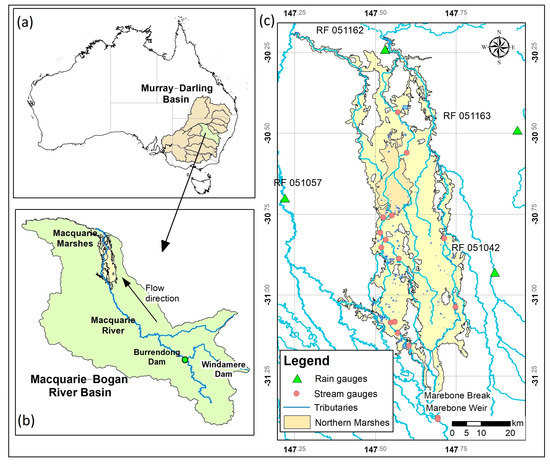
Figure 2.
The location of the study area, Macquarie Marshes, NSW, Australia. (a) The location of the Murray-Darling Basin in Australia. (b) The location of the Macquarie Marshes in the Macquaire-Bogan River Basin. (c) The Macquarie Marshes with tributaries and the locations of rain and stream gauges.
This area receives an average annual rainfall of 400–500 mm, but experiences very high evapotranspiration rates with average annual panevaporation rates of 1800–2400 mm. The average temperature varies from 2–3 °C in winter to 30–36 °C in summer [64]. The Marshes were nurtured by natural flows from the Macquarie River until the 1960s. These natural flows were dependent on rainfall. However, the flows to the Marshes have been significantly reduced, due to the diversions for agricultural and municipal water demands following the Burrendong and Windamere Dams becoming operational in 1967 and 1984 [69,70]. These water diversions have significantly affected streamflow and wetland hydrology [69], as well as directly impacted wetland ecosystem functioning and services, such as maintaining its biodiversity including vegetation health [71], water bird breeding events [67,72,73] and fish populations [74]. The ecological condition of the wetlands declined to critical levels during the prolonged Millennium drought from 2000 to 2009 [71]. In response to this ecological decline, environmental water management plans were implemented and developed for the Macquarie Marshes to increase the flows to the Marshes [66] and its natural ecosystem. These initiatives include the Water Act of 2007, the MDB plan, and provisions to purchase water licenses back for environmental discharges [75]. Details on the Water Act and the Basin plan can be found at https://www.mdba.gov.au/about-us/governance/water-act (accessed on 30 July 2020).
The NSW Department of Planning and Environment (DPIE) developed an inundation mapping product for this area [76] based on the method proposed by Thomas et al. [13]. This product consists of 73 Landsat 7- and 8-based inundation maps of the Marshes from 11 August 2014 to 3 April 2019 at the time of writing this paper. The work presented in this paper expands the dataset from 27 May 1987 to 27 September 2020 and builds a much denser time-series of inundation maps over the area. The proposed method can be easily expanded over future datasets when they are available on the GEE.
3.2. Datasets
Landsat imagery was the main dataset used in this study. Other geospatial, climatic, hydrologic, and vegetation datasets were used for validation and comparisons. A summary of the datasets used in this study is provided in Table 1.

Table 1.
Datasets Used in This Study.
Geometrically corrected, ready-to-use Landsat 5 Thematic Mapper (TM), Landsat 7 Enhanced Thematic Mapper (ETM+), Landsat 8 Operational Land Imager (OLI), and Thermal Infrared Sensor (TIRS) surface reflectance (SR) image collections available in GEE [77] are used in this work to map wetland inundation over the Marshes. Surface reflectance (SR) data are corrected for atmospheric conditions, including aerosol scattering, thin clouds, water vapour and haze effects; therefore, they facilitate the detection and characterisation of changes on the Earth surface. Fisher et al. [78] suggested that water indices developed by using surface reflectance datasets are more useful compared to the ones developed using top-of-atmosphere (TOA) reflectance data. Landsat 5 and 7 surface reflectance datasets were atmospherically corrected using the Landsat Ecosystem Disturbance Adaptive Processing System (LEDAPS) [79,80] and Landsat 8 data using the Land Surface Reflectance Code (LaSRC) [81,82]. Details of the band characteristics of Landsat datasets used in this study are shown in Appendix A. The number of available images per year varies depending on temporal resolution, the combined availability of Landsat imagery, and other environmental conditions.
Inundation maps developed by Thomas et al. [13] were used as a reference dataset in collecting training samples and for validation of the results. Note that the mapping algorithm by Thomas et al. [13] was adapted to develop the wetland inundation maps by the DPIE from 2014 to 2019 using Landsat data. Here, NDWIXu masked by the sum of bands 4, 5, and 7 (sum457) was used to detect water and mixed pixels. Vegetation was classified using an unsupervised classification of a composite image comprising two dates representing vegetation senescence and green growth, transformed into two contrasting vegetation indices, NDVI and NDIB7/B4.
High-spatial resolution aerial images (https://www.spatial.nsw.gov.au, accessed on 15 November 2020) were used to assess the accuracy of the time-record of inundation maps developed by the RaFMIC method. The high-resolution (~50 cm) aerial image dataset acquired by the NSW Spatial Services and high-spatial resolution (<2 m) Google Earth images over the Marshes area collected over multiple dates were used for the validation and accuracy assessments. Further, Sentinel-2 natural colour composites (10 m spatial resolution) for three inundation scenarios under different flood conditions (e.g., 21 August 2016 (high-flood), 9 March 2017 (moderate flood), and 12 February 2019 (dry)), surface water mapping products such as the Water Observations from Space (WOfS) dataset developed by Geoscience Australia, vegetation survey maps [83], and the inundation maps produced by the DPIE [76] were used for the comparison and analysis of the results.
The fluctuation of the total inundated area over the Marshes was compared against the stream discharge data from the study site (https://realtimedata.waternsw.com.au, accessed on 10 December 2020), as well as rainfall data from rain gauges (http://www.bom.gov.au, accessed on 10 November 2020) and the Precipitation Estimation from Remotely Sensed Information using Artificial Neural Networks (PERSIANN) product [84,85]. Here, the daily PERSIANN-Climate Data Record (PERSIANN-CDR) product [86], obtained from the GEE Data Catalog, was used to complement rainfall data from the gauges considering its large spatial areal coverage.
3.3. Applying the Inundation Mapping Algorithm over the Study Area
The mapping algorithm was applied to the Macquarie Marshes area. Inundation maps developed by Thomas et al. [13], high spatial resolution (~50 cm) aerial images obtained from the NSW Spatial Services, vegetation survey maps [83], Landsat natural colour composites, and SWIR-I bands were used as reference data in training and validating the random forest classification algorithm. For each class, over 50 training polygons were created to assure sufficient training samples. The training polygons varied in size from ~4000 m2 to ~2 km2. The high-spatial resolution GEE base map was also used to verify open surface water bodies and tributaries when collecting the training samples.
3.4. Accuracy Assessment
The accuracy of the inundation maps produced by RaFMIC was assessed using (i) high-spatial resolution Google Earth imagery and (ii) very high-spatial resolution airborne imagery. Five high-resolution (~2 m) scenes captured from Google Earth historic images (see Table 1) were used with thirty random points selected on each scene. A 30-m radius buffer was created for each point by considering the spatial resolution of Landsat imagery. Landsat 7 ETM+ data consists of stripes with no data after 2003 due to the failure in the Scan Line Corrector (SLC), and hence points plotted on these data gaps were omitted from this analysis. The true inundation status at each point was obtained by the visual inspection. Here, a point was considered as ‘inundated’ if 50% or more of the 30 m buffer zone was inundated [87,88]. The scenes captured from Google Earth imagery were selected from the Northern Marshes where most inundation events occurred. As the extent of this focused mapping area was approximately 2 km2, the validation points were generated randomly (i.e., simple randomisation) without any particular stratification over the extents covered by the captured Google Earth scenes.
Due to the smaller extent captured with Google Earth imagery, the accuracy of inundation maps was further assessed by comparing them against high-spatial resolution (50 cm) airborne data obtained from NSW Spatial Services from the airborne campaigns conducted in 2008 and 2013 (Table 1). In this airborne dataset, the entire Macquarie Marshes area was covered by six main regions, i.e., (i) Canonba, (ii) Carinda, (iii) Geera, (iv) Hermidon, (v) Mount Harris, and (vi) Quambone (Figure 3). For the accuracy assessment, airborne data over the Quambone and Mount Harris regions were mainly used, since they cover most of the Macquarie Marshes area. Two hundred validation points with 30 m buffers were created over the Macquarie Marshes area for both 2008 and 2013. Of these 200 points, 100 were placed on inundated areas, and the other 100 were placed on noninundated areas of the classified image taken from the same month as the aerial image.
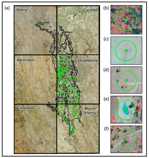
Figure 3.
(a) The six regions of airborne surveys with their 50 cm spatial resolution natural colour composites in April 2013 over the Macquarie Marshes. Two hundred validation points are overlaid on the Quambone and Mount Harris tiles. (b–f) show examples for the stratified points and 30 m buffers over different land use classes (shown in 432 false colour composites where 4 is NIR, 3 is red, and 2 is green band). Here, point (b) is located on an inundated woodland wetland, (c) on a noninundated cultivated land, (d) on a noninundated grassland, (e) on an open water body, and (f) on a noninundated woodland wetland.
The true inundation status was extracted by visual comparison of the 50 cm resolution true colour airborne composites at a high zoom-level. The status was deemed as ‘inundated’ only if more than 50% of the buffer area was inundated in the airborne data. The accuracy of the classification was assessed by comparing the true (observed from airborne data) and classified values.
3.5. Additional Assessment
The soundness of the results was further assessed and validated using existing inundation maps, as well as hydrometeorological and vegetation datasets. The inundation maps and the temporal probability of inundation over the area were compared against streamflow, precipitation, vegetation survey maps, and existing wetland inundation maps to perform a preliminary assessment of the relationship between inundation dynamics and ecohydrological responses. These analyses provide insights for various uses of the inundation datasets to evaluate ecohydrological responses of wetland systems under various inundation conditions.
The inundations maps from RaFMIC were compared against available surface water and inundation mapping products to examine how our mapping algorithm captures wetland inundation under different hydrologic conditions. Here, the inundation maps were first compared against the DEA WOfS daily water observation products at high and low flood events (on 7 September 2010 and 14 November 2014, respectively), and then against the inundation maps developed by Thomas et al. [13] and the DPIE, to see the agreement between the inundation patterns as captured by the three products. Then, the frequency of inundation at each pixel was calculated separately for the Landsat 5-, 7-, and 8-based inundation maps to produce inundation probability maps. The frequency of inundation was compared against key wetlands/storage units determined from a large-scale fine resolution 1D/2D floodplain hydrodynamic model [89]. It is expected that the distribution and location of these key storage units indicating highly inundated areas, i.e., individual dryland wetlands located within the Marshes, should be in agreement with the frequently inundated areas shown from our mapping results.
The temporal trend of the total inundated areas captured from 1987 to 2019 was compared against time-series of streamflow, precipitation, and NDVI to examine the consistency between inundation and hydrological input to the Marshes and the vegetation responses following inundation events. The stream discharge at the inlet to the Marshes (i.e., Marebone Weir and Marebone Break) (Figure 2) was used in this comparison, as it can be considered as a good indicator of the major flows into the Marshes. Thirty-day cumulative discharge was used in this comparison in view of the lag time between stream inflow and inundation reaching through the Marshes [90]. Rainfall data from both PERSIANN-CDR products and rain gauges (# 051042 and # 051057) was used considering differences between in-situ and remote sensing observation and areal extent of precipitation over the study area. The vegetation survey maps created by the NSW Office of Environment and Heritage [83] based on the airborne surveys conducted in 1991, 2008, and 2013 were used to further examine the vegetation response with the inundation dynamics and its change condition.
4. Results
4.1. Training and Validation of the Random Forest Model
In general, the random forest algorithms for the Landsat 5, 7, and 8 collections yielded a good validating accuracy when tested with 10 trees. With each of the three Landsat datasets, an overall accuracy of over 95% was observed. The overall model accuracies calculated by the GEE for 2 to 15 trees are given in the Supplementary Materials.
4.2. Accuracy Assessment of Inundation Maps and Comparison with Available Datasets
The results of the comparison of RaFMIC inundation maps against Google Earth imagery are given in Table 2, along with a summary of the number of random points used with each image. Table 3 shows the detailed confusion matrix of the comparison of inundation maps against the high-spatial resolution airborne datasets (see Figure 3). The comparison between inundation maps and Google Earth Images showed an average accuracy of 91.6% (Table 2), and 50 cm spatial resolution aerial imagery (obtained from NSW Spatial Services) showed an average accuracy of 89% (Table 3).
Table 2.
Results of the Comparison between High Spatial Resolution Imagery and Inundation Maps.
Table 3.
Confusion Matrix for the Accuracy Assessment of Inundation Maps using 2008 and 2013 High Spatial Resolution Airborne Imagery Obtained from the NSW Spatial Services.
Inundation maps from RaFMIC under three inundation scenarios, i.e., high flood, moderate flood, and dry conditions (on 15 August 2016, 11 March 2017, and 13 February 2019, respectively) are shown in Figure 4. The maps show the Northern Marshes (Figure 2) as the most frequently inundated region, with the inundated area generally expanding from the Northern Marshes to the surrounding areas. In Figure 4, the inundation maps produced by RaFMIC were compared against the Sentinel-2 natural colour composites of 10 m spatial resolution for a visual comparison. The dark greenish colour of the Sentinel-2 natural colour composites shows the inundated areas whereas the brownish areas show the dryland. For the Sentinel-2, images from the closest available dates (21 August 2016, 9 March 2017, and 12 February 2019) were chosen for this comparison. They show good agreement with the inundation maps, despite the slight difference in selected dates.
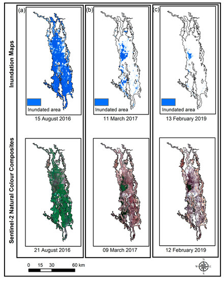
Figure 4.
A comparison of the inundation maps of three inundation scenarios derived from Landsat 8 on (a) 15 August 2016, (b) 11 March 2017, and (c) 12 February 2019 with Sentinel-2 derived natural colour composites of the closest available cloud-free dates.
Figure 5 shows a comparison between inundation maps of surface water mapped by the DPIE, DEA WOfS and RaFMIC created at two inundation scenarios. A larger extent of inundation was observed on 2 October 2016 than on 14 November 2014. It is evident that there is a good agreement between the wetland inundation maps developed by the DPIE and the results of the RaFMIC method. The WOfS dataset has not captured the detailed wetland inundation of this area (Figure 5b,e), especially over the Northern Marshes where frequent inundation takes place. Similarly, the European Commission’s global surface water mapping project (https://global-surface-water.appspot.com, accessed on 15 December 2020) also could not capture wetland inundation in detail. It is noteworthy to mention that the WOfs and European Commission’s global surface water datasets were developed mainly with the aim of providing continental- and global-scale ‘open surface water’ dynamics, respectively, but these products might not always be successful in mapping complex wetland inundation dynamics with mixed responses from vegetation and dissolved matter [30].
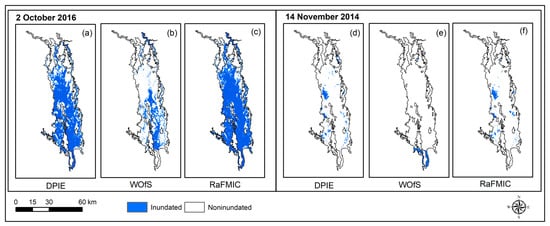
Figure 5.
Comparison between inundation maps developed by the NSW DPIE, DEA WOfs project and inundation maps created in this study using RaFMIC model on (a–c) a high-flood event (2 October 2016) and (d–f) a low-flood event (14 November 2014).
4.3. Characteristics of the Inundated Areas as Mapped from Different Land Cover Classes
The RaFMIC method to map wetland inundation relies on the ability of spectral indices and spectral bands, which are capable of detecting water and vegetation, to collectively capture wetland inundation dynamics. To demonstrate this, Figure 6 shows point-scale spectral signatures and spectral indices observed on 19 September 2017 for four representative land use/land cover classes (inundated vegetation, dryland, noninundated vegetation, and open water bodies) whose locations are shown in Figure 6a. Figure 6b shows the spectral signatures of Landsat 8 SR bands 1 to 7 extracted from the GEE (see Appendix A for band descriptions). Here, distinct peaks can be seen on the SWIR range (B6) on dryland, but open water shows lower values due to high absorption from water. However, some slightly high NIR (B5) values (~0.1) can be seen from water-dominated pixels (e.g., P7, P8), mostly due to mixed responses from vegetation and water or due to phytoplankton in water. Figure 6c shows the NDVI, EVI, NDWIGao, NDWIXu, and SAVI values of these eight points. Each pair of points on the same land use class showed similar patterns to each other, with the exceptions of P7 (river) and P8 (water body). The spectral indices were able to capture distinct properties of the land use classes compared to the spectral bands alone. For example, dryland showed relatively low values for vegetation indices and negative values for water indices, but high reflectance over all bands. Vegetated areas showed high reflectance in NIR (B5) and SWIR (B6), as well as high values for vegetation indices, but negative water index values.
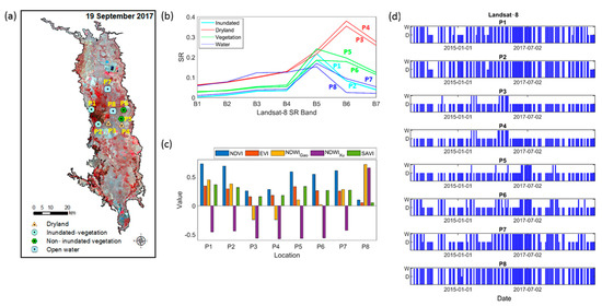
Figure 6.
Point signatures and inundation dynamics of four land use classes over the study area. (a) Locations of eight points over the Landsat 8, 5-4-3 composite on 19 September 2017; (b) spectral signatures of the eight points extracted from Landsat 8 image; (c) index values of NDVI, EVI, NDWIGao, NDWIXu, and SAVI of the eight points extracted from the Landsat 8 image; and (d) the inundation time-series of the eight points (here, W is wet and D is dry). Here, P1 and P2 are inundated vegetation, P3 and P4 are dryland, P5 and P6 are noninundated vegetation, and P7 (river) and P8 (water body) are open water.
Figure 6d shows the temporal inundation dynamics of these eight points as captured by the Landsat 8-based RaFMIC inundation maps. Here, typical inundation dynamics for these land use classes are demonstrated reflecting their onsite biogeophyiscal characteristics. For example, inundated vegetation (P1 and P2) shows variable wet (W) and dry (D) dynamics common to wetland inundation. Overall, it shows strong vegetation signals with relatively high vegetation water contents (Figure 6c), as compared to other land cover types. Dryland (P3 and P4) and noninundated vegetation (P5 and P6) show constantly dry (soil) conditions, with the exception of a few days. The open water body at P8 showed general wet conditions. However, P7 (river) showed some variability between wet and dry status, which could indicate an intermittent river experiencing frequent changes in surface water properties and water signals mixed with vegetation (as indicated by vegetation indices in Figure 6c). For example, the presence of vegetation, organic matter, high turbidity, change in water depths, and the amount of water flows in the channel changed the spectral responses with mixed signals.
4.4. Inundation Change Dynamics: Comparison with Hydrometeorological Conditions
A comparison of the time-record of the inundated area over the Macquarie Marshes with streamflow, precipitation, and NDVI is shown in Figure 7. Overall, the Landsat 5, 7, and 8 sensors show consistent inundation patterns. The mismatches between inundated areas captured by different Landsat missions were mainly caused by different satellite overpass dates. It is evident in Figure 7a,b that the results from the inundation maps show good agreement with the 30-day cumulative discharge at Marebone Weir (site no: 421090) and Marebone Break (site no: 421088). When the inundated area was available from two satellites in Figure 7a, the mean of these two datasets were calculated and shown in Figure 7b for a better comparison between the temporal agreement of the inundated area and the 30-day cumulative discharge. Figure 7a,c show a weaker association between 30-day rainfall and inundation than between Figure 7a,b with the inundation area mainly showing a response to rainfall above a threshold of 50 mm (dashed line). This weaker association arises because the rainfall observations represent rainfall in the vicinity of the Marshes (see Figure 2) and not the rainfall in the upper parts of the Macquarie basin, which is responsible for much of the streamflow. Major peaks in NDVI values (Figure 7d) (~NDVI>0.3) show an agreement with the inundated area similar to rainfall. The NDVI value of 0.3 is plotted (dashed line) in Figure 7d to elucidate this. A careful examination shows a slight delay in the NDVI (i.e., vegetation) response to the inundation events after a dry period, as shown in the inset figure related to Figure 7d. From Figure 7, it is evident that streamflow and heavy rainfall events are main drivers of the inundated area over the Marshes.
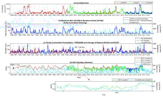
Figure 7.
(a) Inundated area within Macquarie Marshes as captured by the Landsat 5-, 7-, and 8-based inundation maps; (b) 30-day cumulative discharge at Marebone Weir and Marebone Break (# 421,090 and # 421088); (c) 30-day cumulative precipitation across the study area captured by PERSIANN data and rainfall stations (# 051042 and # 051057) with inundated area; and (d) average NDVI over the northern Marshes with inundated area as captured by the Landsat 5-, 7-, and 8-based products.
4.5. Spatial Patterns of Temporal Inundation Dynamics
Figure 8a–c show the probability of inundation over each 30 × 30 m pixel, as captured from the RaFMIC inundation maps over the study time period. Here, 214 Landsat 5 scenes, 245 Landsat 7 scenes, and 95 Landsat 8 scenes have been used to calculate the probability of inundation over the time. The probabilities of the inundation maps were overlaid with the wetlands/storage units where frequent inundation occurs based on the MIKE Flood hydrodynamic model [89]. These storage areas show a good agreement with the inundation probabilities. A good consistency between the hydraulic simulation and our inundation maps provides additional support for our mapping results. Inundation probability maps developed using all three Landsat image collections used in this study (i.e., Landsat 5, 7, and 8) showed very similar spatial patterns despite the differences in their time periods and sensor specifications. When zoomed-in, a good agreement can be seen between temporal inundation dynamics (Figure 8d) and woodland vegetation, as shown by a high-spatial resolution natural colour composite (Figure 8e). This preliminary comparison suggests that the inundation maps developed here can be highly useful in evaluating the vegetation change conditions over the Marshes.
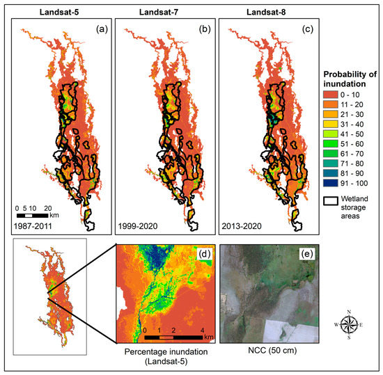
Figure 8.
Probability of inundation over the Macquarie Marshes as captured by the inundation maps based on (a) Landsat 5, (b) Landsat 7, and (c) Landsat 8 SR image collections. Wetland storage units derived based on the hydrodynamic model (MIKE Flood) [89] are overlaid over the probability of inundation maps. Probability of inundation and a high-spatial resolution natural colour composite created using the NSW Spatial Services airborne data are shown in (d) and (e), respectively, for an area in Northern Marshes.
Figure 9a,b show wet and dry year inundation dynamics captured by RaFMIC. The year 2019 was the driest and warmest year on record for NSW, while 2016 was classified as a wet and warm year in NSW [91]. Both annual discharge data from the inlet to the Marshes (i.e., Marebone Weir station) (Figure 9c) and annual rainfall data from the weather stations # 051042 and # 051057 (Figure 9d) confirm 2016 as a wet year (i.e., with the total rainfall and annual discharge much higher than the overall mean) and 2019 as a dry year (i.e., less than mean annual precipitation and stream discharge). These wet and dry conditions are evident in the probability of inundation calculated by the Landsat 8-based inundation maps available in 2016 and 2019, respectively (Figure 9a,b). Figure 9a shows a mean inundation probability of 34% with a standard deviation of 17% in 2016, whereas Figure 9b shows a mean of 3% with a standard deviation of 3% in 2019. In 2016, 1314 km2 (i.e., ~66% of the entire Marshes area) had an inundation probability of over 25%, whereas in 2019, this value reduces to 74 km2 (i.e., ~4% of the entire Marshes area).
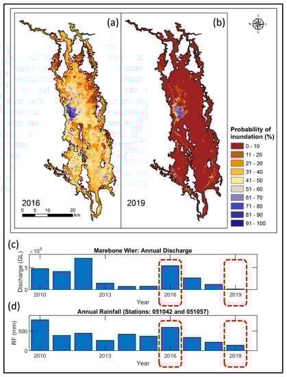
Figure 9.
Inundation dynamics (percentage wet count) over the Macquarie Marshes in a (a) wet (2016) and a (b) dry (2019) year as captured by the Landsat 8-based inundation maps. (c) The annual discharge at Marebone Wier and (d) the annual rainfall of the average of stations 051042 and 051057 show the wetness in 2016 and dryness in 2019 over the study area.
Figure 10 shows a comparison between the vegetation mapping carried out in 1991, 2008, and 2013 [83] with the inundation maps. The inundation probability (Figure 10a–c) was calculated based on the inundation maps of four months, prior to the airborne data collections conducted for vegetation mapping. Landsat derived mean NDVI maps for these periods are shown in Figure 10g–i. A good agreement can be seen between the frequently inundated area (for both dry and wet conditions shown in Figure 10a–c) with river red gum woodland and forest (Figure 10d–f). An intrusion of invasive vegetation into the semipermanent wetlands can be seen in 2008, reducing the spatial extent of semi-permanent wetlands (Figure 10e). A low inundation probability can be observed in 2008 (mean areal probability=11.6%, Figure 10a) compared to 1991 (mean areal probability=19.4%, Figure 10b). However, a re-expansion of semipermanent wetlands can be observed over the Northern Marshes by 2013 (Figure 10f), probably as a response to flood events over the area which occurred between 2010 and 2012 (Figure 10c).
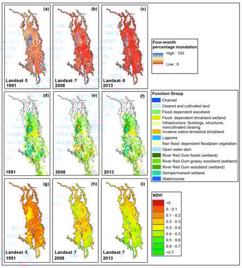
Figure 10.
Percentage temporal inundation over the Macquarie Marshes four months prior to vegetation aerial surveys, i.e., (a) October 1990 to January 1991 (Landsat 5-based), (b) April to July 2008 (Landsat 7-based), and (c) June to September 2013 (Landsat 8-based). Vegetation surveys were conducted in (d) 1991, (e) 2008, and (f) 2013 (Bowen et al., 2019). NDVI maps of the months in which vegetation surveys were carried out are shown in (g–i).
5. Discussion
The inundation maps developed using RaFMIC method showed good accuracy when compared against high-resolution Google Earth and aerial imagery. The thick algal blooms covering larger extents [92,93] also made it sometimes difficult to identify the true inundation statuses of some points. Lack of field data was a major limitation in carrying out an accuracy assessment against reliable field observations. The comparisons with existing inundation maps, hydrological, meteorological, and vegetation datasets were used for a deeper assessment of the results. The results showed a good agreement with available inundation maps, storage units (i.e., key wetlands within the Marshes), streamflow, and meteorological data (Figure 5, Figure 6, Figure 7, Figure 8 and Figure 9). The vegetation dynamics (as observed by the NDVI) and vegetation maps based on field surveys [83] also show good spatial and temporal agreement with the inundation maps developed in this study.
These results suggest that the RaFMIC method is robust. Moreover, RaFMIC does not need separate pre- and postflood imagery for each inundation event or setting up manual thresholds. The inundation maps prepared by Thomas et al. [13] were used as reference maps for the training and validation of the random forest model to capture a range of water signals mixed with vegetation. Field data or information captured by high-spatial resolution imagery can be used as alternatives when reference maps are not available. Once the classifier is trained, it can be applied over the entire time-series of images, including the future datasets. This approach allows straightforward modification and improvement, such as addition of indices and the use of different combinations of indices. Flexibility, semiautomation, and time-effectiveness are the key features of the GEE-based RaFMIC algorithm that make it the preferred choice over existing methods.
In future studies, the algorithm can be further improved upon by adding more combinations of indices such as the Tasselled Cap Index [94] or Topographic Wetness Indices [95]. Such indices might be capable of capturing vital training information to further improve the classification accuracy. Although random forest provides a robust method, the feature randomness of the algorithm can cause some uncertainties. These uncertainties can be minimised by using a greater number of trees, but this increases the computational load. Therefore, it would be worthwhile to compare the RaFMIC method against other GEE-based machine learning algorithms such as the Classification and Regression Trees (CART). The GEE provides a good platform for such testing and modification, with its inbuilt datasets, algorithms, and computation facilities. This method can be easily applied to other wetland areas to create a time-series of inundation maps when reference data (in the form of field data, previous inundation maps, or high-spatial resolution images) are available for training and validating the model. It would be useful to test these algorithms with datasets such as Moderate Resolution Imaging Spectroradiometer (MODIS) and Sentinel-2 data to test the effects of image spatial resolution on wetland mapping. In particular, it would be worthwhile to inspect how Sentinel-2 data (~10 m resolution) can detect subpixel inundation compared to Landsat-derived inundation maps.
Testing Sentinel-1 data for inundation mapping is useful during high-flood events where optical/thermal data-based methods are often ineffective due to thick cloud cover. A dense time-series of inundation maps, along with a high-spatial resolution DEM, can provide baseline information to quantify changes over the last three decades, to better understand landscape-scale hydroperiod and inundation change dynamics. Moreover, such a time-series of inundation maps is a major requisite in developing a data-driven model to characterize ecohydrological changes in the Marshes and in the vulnerability and conditional assessment of wetland ecosystems (e.g., vegetation, bird, and fish breeding) with respect to water availability and other environmental stressors across spatial and temporal scales. Further, a series of inundation maps, and the information derived from it, could be used to assist decision support for environmental water releases to the Marshes.
6. Conclusions
A robust method, RaFMIC, was developed in this study to map inundation dynamics of inland wetlands by using the strengths of the random forest algorithm, multi-index classification, and the Google Earth Engine. The RaFMIC method provides a rapid, semiautomated approach to generate a long-term time-record of wetland inundation maps, which do not require predefined thresholds or pre- and postinundation images of each inundation event, unlike many of the previous wetland mapping methods. The method was tested over the Macquarie Marshes, Australia, to create a temporally dense, three-decadal time record of inundation maps using the Landsat 5, 7, and 8 image collections. The results showed good accuracy when compared against high-spatial resolution imagery, and displayed a good agreement with streamflow, rainfall, and vegetation data. Further, the maps developed in this study were used to identify frequently inundated, key individual wetlands over the Marshes. The time-record of inundation maps developed in this study can be used to improve wetland inventory, analyse wetland ecohydrological responses to changes in inundation regime due to water management and climate change, and help site-specific decision support framework. This approach can be readily applied to other inland wetland regions to effectively build a long-term time-record of inundation maps through a remotely sensed data-driven approach.
Supplementary Materials
The following supporting information can be downloaded at: https://www.mdpi.com/article/10.3390/rs15051263/s1, Overall accuracies of the model validations at different numbers of trees, calculated with GEE.
Author Contributions
Conceptualisation, I.P.S., I.-Y.Y. and G.A.K.; methodology, I.P.S. and I.-Y.Y.; software, I.P.S.; validation, I.P.S. and I.-Y.Y.; formal analysis, I.P.S.; investigation, I.P.S. and I.-Y.Y.; resources, I.-Y.Y. and G.A.K.; data curation, I.P.S. and I.-Y.Y.; writing—original draft preparation, I.P.S.; writing—review and editing, I.P.S., I.-Y.Y. and G.A.K.; supervision, I.-Y.Y. and G.A.K.; project administration, G.A.K. and I.-Y.Y.; funding acquisition, I.-Y.Y. and G.A.K. All authors have read and agreed to the published version of the manuscript.
Funding
This research was funded by the Australian Research Council (ARC), Discovery Project Grant DP190100113.
Data Availability Statement
Sources of the datasets used in this study are provided in the Datasets section. The inundation maps developed in this study and the GEE script are available on request from the corresponding author.
Acknowledgments
Authors wish to thank the Li Wen from the NSW DPIE for his assistance, NSW Spatial Services for providing data, and Ashane M. Fernando from Wayamba University of Sri Lanka for his assistance with the GEE JavaScript.
Conflicts of Interest
The authors declare no conflict of interest.
Appendix A
Table A1.
Band Characteristics of Landsat and Sentinel Data Used in this Study (only the bands used in this work are mentioned ere). (Source: Earth Engine Data Catalog [69]).
Table A1.
Band Characteristics of Landsat and Sentinel Data Used in this Study (only the bands used in this work are mentioned ere). (Source: Earth Engine Data Catalog [69]).
| Band Name | Description | Wavelength | Spatial Resolution |
|---|---|---|---|
| USGS Landsat 5 Surface Reflectance Tier 1 | |||
| B1 | Band 1 (blue) surface reflectance | 0.45–0.52 μm | 30 m |
| B2 | Band 2 (green) surface reflectance | 0.52–0.60 μm | 30 m |
| B3 | Band 3 (red) surface reflectance | 0.63–0.69 μm | 30 m |
| B4 | Band 4 (NIR) surface reflectance | 0.77–0.90 μm | 30 m |
| B5 | Band 5 (SWIR 1) surface reflectance | 1.55–1.75 μm | 30 m |
| B7 | Band 7 (SWIR 2) surface reflectance | 2.08–2.35 μm | 30 m |
| USGS Landsat 7 Surface Reflectance Tier 1 | |||
| B1 | Band 1 (blue) surface reflectance | 0.45–0.52 μm | 30 m |
| B2 | Band 2 (green) surface reflectance | 0.52–0.60 μm | 30 m |
| B3 | Band 3 (red) surface reflectance | 0.63–0.69 μm | 30 m |
| B4 | Band 4 (NIR) surface reflectance | 0.77–0.90 μm | 30 m |
| B5 | Band 5 (SWIR 1) surface reflectance | 1.55–1.75 μm | 30 m |
| B7 | Band 7 (SWIR 2) surface reflectance | 2.08–2.35 μm | 30 m |
| USGS Landsat 8 Surface Reflectance Tier 1 | |||
| B2 | Band 2 (blue) surface reflectance | 0.452–0.512 μm | 30 m |
| B3 | Band 3 (green) surface reflectance | 0.533–0.590 μm | 30 m |
| B4 | Band 4 (red) surface reflectance | 0.636–0.673 μm | 30 m |
| B5 | Band 5 (NIR) surface reflectance | 0.851–0.879 μm | 30 m |
| B6 | Band 6 (SWIR 1) surface reflectance | 1.566–1.651 μm | 30 m |
| B7 | Band 7 (SWIR 2) surface reflectance | 2.107–2.294 μm | 30 m |
References
- Gardner, R.C.; Davidson, N.C. The Ramsar Convention. In Wetlands; Springer: Berlin/Heidelberg, Germany, 2011; pp. 189–203. [Google Scholar]
- Matthews, G.V.T. The Ramsar Convention on Wetlands: its History and Development; Ramsar Convention Bureau: Gland, Switzerland, 1993. [Google Scholar]
- Department of Agriculture Water and Environment, Australia. Water Policy and Resources. Available online: https://www.environment.gov.au/wetlands (accessed on 29 September 2020).
- Gibbs, J.P. Importance of small wetlands for the persistence of local populations of wetland-associated animals. Wetlands 1993, 13, 25–31. [Google Scholar]
- Silvius, M.; Oneka, M.; Verhagen, A. Wetlands: lifeline for people at the edge. Phys. Chem. Earth Part B Hydrol. Ocean. Atmos. 2000, 25, 645–652. [Google Scholar]
- Williams, J.D.; Dodd, C.K., Jr. Importance of wetlands to endangered and threatened species. In Wetland Functions and Values: The State of Our Understanding; American Water Resources Association: Woodbridge, VA, USA, 1978; pp. 565–575. [Google Scholar]
- Chiu, M.-C.; Leigh, C.; Mazor, R.; Cid, N.; Resh, V. Anthropogenic threats to intermittent rivers and ephemeral streams. In Intermittent Rivers and Ephemeral Streams; Elsevier: Amsterdam, The Netherlands, 2017; pp. 433–454. [Google Scholar]
- Kobayashi, T.; Ryder, D.S.; Ralph, T.J.; Mazumder, D.; Saintilan, N.; Iles, J.; Knowles, L.; Thomas, R.; Hunter, S. Longitudinal spatial variation in ecological conditions in an in-channel floodplain river system during flow pulses. River Res. Appl. 2011, 27, 461–472. [Google Scholar] [CrossRef]
- Randklev, C.R.; Miller, T.; Hart, M.; Morton, J.; Johnson, N.A.; Skow, K.; Inoue, K.; Tsakiris, E.T.; Oetker, S.; Smith, R. A semi-arid river in distress: Contributing factors and recovery solutions for three imperiled freshwater mussels (Family Unionidae) endemic to the Rio Grande basin in North America. Sci. Total Environ. 2018, 631, 733–744. [Google Scholar] [CrossRef]
- Robinove, C.J. Interpretation of a Landsat image of an unusual flood phenomenon in Australia. Remote Sens. Environ. 1978, 7, 219–225. [Google Scholar]
- Smith, L.C. Satellite remote sensing of river inundation area, stage, and discharge: A review. Hydrol. Process. 1997, 11, 1427–1439. [Google Scholar]
- Wulder, M.A.; Loveland, T.R.; Roy, D.P.; Crawford, C.J.; Masek, J.G.; Woodcock, C.E.; Allen, R.G.; Anderson, M.C.; Belward, A.S.; Cohen, W.B. Current status of Landsat program, science, and applications. Remote Sens. Environ. 2019, 225, 127–147. [Google Scholar]
- Thomas, R.F.; Kingsford, R.T.; Lu, Y.; Cox, S.J.; Sims, N.C.; Hunter, S.J. Mapping inundation in the heterogeneous floodplain wetlands of the Macquarie Marshes, using Landsat Thematic Mapper. J. Hydrol. 2015, 524, 194–213. [Google Scholar]
- Tulbure, M.G.; Broich, M.; Stehman, S.V.; Kommareddy, A. Surface water extent dynamics from three decades of seasonally continuous Landsat time series at subcontinental scale in a semi-arid region. Remote Sens. Environ. 2016, 178, 142–157. [Google Scholar]
- Heimhuber, V.; Tulbure, M.; Broich, M. Modeling multidecadal surface water inundation dynamics and key drivers on large river basin scale using multiple time series of E arth-observation and river flow data. Water Resour. Res. 2017, 53, 1251–1269. [Google Scholar] [CrossRef]
- Senay, G.B.; Schauer, M.; Friedrichs, M.; Velpuri, N.M.; Singh, R.K. Satellite-based water use dynamics using historical Landsat data (1984–2014) in the southwestern United States. Remote Sens. Environ. 2017, 202, 98–112. [Google Scholar] [CrossRef]
- Mueller, N.; Lewis, A.; Roberts, D.; Ring, S.; Melrose, R.; Sixsmith, J.; Lymburner, L.; McIntyre, A.; Tan, P.; Curnow, S. Water observations from space: Mapping surface water from 25 years of Landsat imagery across Australia. Remote Sens. Environ. 2016, 174, 341–352. [Google Scholar] [CrossRef]
- Donchyts, G.; Baart, F.; Winsemius, H.; Gorelick, N.; Kwadijk, J.; Van De Giesen, N. Earth’s surface water change over the past 30 years. Nat. Clim. Chang. 2016, 6, 810–813. [Google Scholar] [CrossRef]
- Pekel, J.-F.; Cottam, A.; Gorelick, N.; Belward, A.S. High-resolution mapping of global surface water and its long-term changes. Nature 2016, 540, 418–422. [Google Scholar] [CrossRef] [PubMed]
- Frazier, P.S.; Page, K.J. Water body detection and delineation with Landsat TM data. Photogramm. Eng. Remote Sens. 2000, 66, 1461–1468. [Google Scholar]
- Tucker, C.J. Red and photographic infrared linear combinations for monitoring vegetation. Remote Sens. Environ. 1979, 8, 127–150. [Google Scholar] [CrossRef]
- Gao, B.-C. NDWI—A normalized difference water index for remote sensing of vegetation liquid water from space. Remote Sens. Environ. 1996, 58, 257–266. [Google Scholar] [CrossRef]
- McFeeters, S.K. The use of the Normalized Difference Water Index (NDWI) in the delineation of open water features. Int. J. Remote Sens. 1996, 17, 1425–1432. [Google Scholar] [CrossRef]
- Xu, H. Modification of normalised difference water index (NDWI) to enhance open water features in remotely sensed imagery. Int. J. Remote Sens. 2006, 27, 3025–3033. [Google Scholar] [CrossRef]
- Pope, R.M.; Fry, E.S. Absorption spectrum (380–700 nm) of pure water. II. Integrating cavity measurements. Appl. Opt. 1997, 36, 8710–8723. [Google Scholar] [CrossRef]
- Smith, R.C.; Baker, K.S. Optical properties of the clearest natural waters (200–800 nm). Appl. Opt. 1981, 20, 177–184. [Google Scholar] [CrossRef]
- Hogg, A.; Holland, J. An evaluation of DEMs derived from LiDAR and photogrammetry for wetland mapping. For. Chron. 2008, 84, 840–849. [Google Scholar] [CrossRef]
- Lang, M.; McCarty, G.; Oesterling, R.; Yeo, I.-Y. Topographic metrics for improved mapping of forested wetlands. Wetlands 2013, 33, 141–155. [Google Scholar] [CrossRef]
- Millard, K.; Richardson, M. Wetland mapping with LiDAR derivatives, SAR polarimetric decompositions, and LiDAR–SAR fusion using a random forest classifier. Can. J. Remote Sens. 2013, 39, 290–307. [Google Scholar] [CrossRef]
- Krause, C.E.; Newey, V.; Alger, M.J.; Lymburner, L. Mapping and monitoring the multi-decadal dynamics of Australia’s open waterbodies using Landsat. Remote Sens. 2021, 13, 1437. [Google Scholar] [CrossRef]
- Australian Government. DEA Waterbodies. Available online: https://cmi.ga.gov.au/data-products/dea/693/dea-waterbodies-landsat#details (accessed on 1 May 2022).
- Yeo, I.-Y.; Lang, M.; Vermote, E. Improved understanding of suspended sediment transport process using multi-temporal Landsat data: A case study from the Old Woman Creek Estuary (Ohio). IEEE J. Sel. Top. Appl. Earth Obs. Remote Sens. 2013, 7, 636–647. [Google Scholar] [CrossRef]
- Huang, X.; Lu, Q.; Zhang, L. A multi-index learning approach for classification of high-resolution remotely sensed images over urban areas. ISPRS J. Photogramm. Remote Sens. 2014, 90, 36–48. [Google Scholar] [CrossRef]
- Tang, Z.; Li, Y.; Gu, Y.; Jiang, W.; Xue, Y.; Hu, Q.; LaGrange, T.; Bishop, A.; Drahota, J.; Li, R. Assessing Nebraska playa wetland inundation status during 1985–2015 using Landsat data and Google Earth Engine. Environ. Monit. Assess. 2016, 188, 654. [Google Scholar] [CrossRef] [PubMed]
- Verpoorter, C.; Kutser, T.; Tranvik, L. Automated mapping of water bodies using Landsat multispectral data. Limnol. Oceanogr. Methods 2012, 10, 1037–1050. [Google Scholar] [CrossRef]
- Araya-López, R.A.; Lopatin, J.; Fassnacht, F.E.; Hernández, H.J. Monitoring Andean high altitude wetlands in central Chile with seasonal optical data: A comparison between Worldview-2 and Sentinel-2 imagery. ISPRS J. Photogramm. Remote Sens. 2018, 145, 213–224. [Google Scholar] [CrossRef]
- Kaplan, G.; Avdan, U. Monthly analysis of wetlands dynamics using remote sensing data. ISPRS Int. J. Geo-Inf. 2018, 7, 411. [Google Scholar] [CrossRef]
- Tung, F.; LeDrew, E. The determination of optimal threshold levels for change detection using various accuracy indexes. Photogramm. Eng. Remote Sens. 1988, 54, 1449–1454. [Google Scholar]
- Huang, C.; Smith, L.C.; Kyzivat, E.D.; Fayne, J.V.; Ming, Y.; Spence, C. Tracking transient boreal wetland inundation with Sentinel-1 SAR: Peace-Athabasca Delta, Alberta and Yukon Flats, Alaska. GIScience Remote Sens. 2022, 59, 1767–1792. [Google Scholar] [CrossRef]
- Sahour, H.; Kemink, K.M.; O’Connell, J. Integrating SAR and optical remote sensing for conservation-targeted wetlands mapping. Remote Sens. 2021, 14, 159. [Google Scholar] [CrossRef]
- Adeli, S.; Salehi, B.; Mahdianpari, M.; Quackenbush, L.J.; Chapman, B. Moving Toward L-Band NASA-ISRO SAR Mission (NISAR) Dense Time Series: Multipolarization Object-Based Classification of Wetlands Using Two Machine Learning Algorithms. Earth Space Sci. 2021, 8, 2021EA001742. [Google Scholar] [CrossRef]
- Fang, H.; Liang, S. Leaf Area Index Models, Reference Module in Earth Systems and Environmental Sciences. Encycl. Ecol. 2014, 2139–2148. [Google Scholar]
- Zhang, F.; Zhou, G. Estimation of vegetation water content using hyperspectral vegetation indices: A comparison of crop water indicators in response to water stress treatments for summer maize. BMC Ecol. 2019, 19, 1–12. [Google Scholar] [CrossRef]
- López-Tapia, S.; Ruiz, P.; Smith, M.; Matthews, J.; Zercher, B.; Sydorenko, L.; Varia, N.; Jin, Y.; Wang, M.; Dunn, J.B. Machine learning with high-resolution aerial imagery and data fusion to improve and automate the detection of wetlands. Int. J. Appl. Earth Obs. Geoinf. 2021, 105, 102581. [Google Scholar] [CrossRef]
- Mallick, J.; Talukdar, S.; Pal, S.; Rahman, A. A novel classifier for improving wetland mapping by integrating image fusion techniques and ensemble machine learning classifiers. Ecol. Inform. 2021, 65, 101426. [Google Scholar] [CrossRef]
- Gemechu, G.F.; Rui, X.; Lu, H. Wetland Change Mapping Using Machine Learning Algorithms, and Their Link with Climate Variation and Economic Growth: A Case Study of Guangling County, China. Sustainability 2021, 14, 439. [Google Scholar] [CrossRef]
- Zhang, L.; Hu, Q.; Tang, Z. Using Sentinel-2 Imagery and Machine Learning Algorithms to Assess the Inundation Status of Nebraska Conservation Easements during 2018–2021. Remote Sens. 2022, 14, 4382. [Google Scholar] [CrossRef]
- Gonzalez-Perez, A.; Abd-Elrahman, A.; Wilkinson, B.; Johnson, D.J.; Carthy, R.R. Deep and Machine Learning Image Classification of Coastal Wetlands Using Unpiloted Aircraft System Multispectral Images and Lidar Datasets. Remote Sens. 2022, 14, 3937. [Google Scholar] [CrossRef]
- Ho, T.K. Random decision forests. In Proceedings of the 3rd International Conference on Document Analysis and Recognition, Montreal, QC, Canada, 14–16 August 1995; pp. 278–282. [Google Scholar]
- Gorelick, N.; Hancher, M.; Dixon, M.; Ilyushchenko, S.; Thau, D.; Moore, R. Google Earth Engine: Planetary-scale geospatial analysis for everyone. Remote Sens. Environ. 2017, 202, 18–27. [Google Scholar] [CrossRef]
- Tamiminia, H.; Salehi, B.; Mahdianpari, M.; Quackenbush, L.; Adeli, S.; Brisco, B. Google Earth Engine for geo-big data applications: A meta-analysis and systematic review. ISPRS J. Photogramm. Remote Sens. 2020, 164, 152–170. [Google Scholar] [CrossRef]
- Ahmed, K.R.; Akter, S. Analysis of landcover change in southwest Bengal delta due to floods by NDVI, NDWI and K-means cluster with Landsat multi-spectral surface reflectance satellite data. Remote Sens. Appl. Soc. Environ. 2017, 8, 168–181. [Google Scholar] [CrossRef]
- Colditz, R.R.; Souza, C.T.; Vazquez, B.; Wickel, A.J.; Ressl, R. Analysis of optimal thresholds for identification of open water using MODIS-derived spectral indices for two coastal wetland systems in Mexico. Int. J. Appl. Earth Obs. Geoinf. 2018, 70, 13–24. [Google Scholar] [CrossRef]
- Szabo, S.; Gácsi, Z.; Balazs, B. Specific features of NDVI, NDWI and MNDWI as reflected in land cover categories. Landsc. Environ. 2016, 10, 194–202. [Google Scholar] [CrossRef]
- Liu, H.Q.; Huete, A. A feedback based modification of the NDVI to minimize canopy background and atmospheric noise. IEEE Trans. Geosci. Remote Sens. 1995, 33, 457–465. [Google Scholar] [CrossRef]
- Huete, A.; Didan, K.; Miura, T.; Rodriguez, E.P.; Gao, X.; Ferreira, L.G. Overview of the radiometric and biophysical performance of the MODIS vegetation indices. Remote Sens. Environ. 2002, 83, 195–213. [Google Scholar] [CrossRef]
- Khaliq, A.; Musci, M.A.; Chiaberge, M. Analyzing relationship between maize height and spectral indices derived from remotely sensed multispectral imagery. In Proceedings of the 2018 IEEE Applied Imagery Pattern Recognition Workshop (AIPR), Washington, DC, USA, 9–11 October 2018; pp. 1–5. [Google Scholar]
- USGS. Landsat Surface Reflectance-Derived Spectral Indices, Landsat Enhanced Vegetation Index. Available online: https://www.usgs.gov/core-science-systems/nli/landsat/landsat-enhanced-vegetation-index?qt-science_support_page_related_con=0#qt-science_support_page_related_con (accessed on 11 December 2020).
- Huete, A.R. A soil-adjusted vegetation index (SAVI). Remote Sens. Environ. 1988, 25, 295–309. [Google Scholar] [CrossRef]
- USGS. Landsat Soil Adjusted Vegetation Index. Available online: https://www.usgs.gov/landsat-missions/landsat-soil-adjusted-vegetation-index (accessed on 20 November 2021).
- Memon, A.A.; Muhammad, S.; Rahman, S.; Haq, M. Flood monitoring and damage assessment using water indices: A case study of Pakistan flood-2012. Egypt. J. Remote Sens. Space Sci. 2015, 18, 99–106. [Google Scholar] [CrossRef]
- Breiman, L. Random forests. Mach. Learn. 2001, 45, 5–32. [Google Scholar] [CrossRef]
- Pal, M. Random forest classifier for remote sensing classification. Int. J. Remote Sens. 2005, 26, 217–222. [Google Scholar] [CrossRef]
- Thomas, R.F.; Ocock, J.F. Macquarie Marshes: Murray-Darling River Basin (Australia). In The Wetland Book; Finlayson, C.M., Milton, G.R., Prentice, R.C., Davidson, N.C., Eds.; Srpinger: Berlin/Heidelberg, Germany, 2018. [Google Scholar]
- McComb, A.J.; Lake, P.S. The Conservation of Australian Wetlands; Surrey Beatty & Sons: Chipping Norton, Australia, 1988. [Google Scholar]
- OEH. Environmental Water Use in New South Wales. Outcomes 2013–14; Office of Environment and Heritage: Sydney, Australia, 2014. [Google Scholar]
- Kingsford, R.; Johnson, W. Impact of water diversions on colonially-nesting waterbirds in the Macquarie Marshes of arid Australia. Colonial Waterbirds 1998, 21, 159–170. [Google Scholar] [CrossRef]
- Kingsford, R.T.; Auld, K.M. Waterbird breeding and environmental flow management in the Macquarie Marshes, arid Australia. River Res. Appl. 2005, 21, 187–200. [Google Scholar] [CrossRef]
- Ren, S.; Kingsford, R.T.; Thomas, R.F. Modelling flow to and inundation of the Macquarie Marshes in arid Australia. Environmetrics 2010, 21, 549–561. [Google Scholar] [CrossRef]
- Ren, S.; Kingsford, R.T. Statistically integrated flow and flood modelling compared to hydrologically integrated quantity and quality model for annual flows in the regulated Macquarie River in arid Australia. Environ. Manag. 2011, 48, 177–188. [Google Scholar] [CrossRef]
- Rogers, K.; Ralph, T.J. Floodplain Wetland Biota in the Murray-Darling Basin: Water and Habitat Requirements; Csiro Publishing: Melbourne, Australia, 2010. [Google Scholar]
- Kingsford, R.T.; Thomas, R.F. The Macquarie Marshes in arid Australia and their waterbirds: a 50-year history of decline. Environ. Manag. 1995, 19, 867–878. [Google Scholar] [CrossRef]
- Kingsford, R.T. Ecological impacts of dams, water diversions and river management on floodplain wetlands in Australia. Austral. Ecol. 2000, 25, 109–127. [Google Scholar] [CrossRef]
- Rayner, T.S.; Jenkins, K.M.; Kingsford, R.T. Small environmental flows, drought and the role of refugia for freshwater fish in the Macquarie Marshes, arid Australia. Ecohydrol. Ecosyst. Land Water Process Interact. Ecohydrogeomorphol. 2009, 2, 440–453. [Google Scholar] [CrossRef]
- Murray-Darling Basin Authority. The Basin Plan. Available online: https://www.mdba.gov.au/basin-plan/plan-murray-darling-basin (accessed on 1 October 2021).
- The Central Resource for Sharing and Enabling Environmental Data in NSW. Inundation Maps for NSW Inland Floodplain Wetlands. Available online: https://datasets.seed.nsw.gov.au/dataset/inundation-maps-for-nsw-inland-floodplain-wetlands (accessed on 20 December 2020).
- Earth Engine Data Catalog. A Planetary-Scale Platform for Earth Science Data & Analysis. Available online: https://developers.google.com/earth-engine/datasets (accessed on 1 September 2020).
- Fisher, A.; Flood, N.; Danaher, T. Comparing Landsat water index methods for automated water classification in eastern Australia. Remote Sens. Environ. 2016, 175, 167–182. [Google Scholar] [CrossRef]
- Vermote, E.; Saleous, N. LEDAPS Surface Reflectance Product Description; University of Maryland, College Park: City of College Park, MD, USA, 2007. [Google Scholar]
- USGS. Landsat 4-7 Collection 1 (C1) Surface Reflectance (LEDAPS) Product Guide; Version 3.0; Department of the Interior, U.S. Geological Survey: Reston, VA, USA, 2020.
- Vermote, E.; Roger, J.-C.; Franch, B.; Skakun, S. LaSRC (Land Surface Reflectance Code): Overview, application and validation using MODIS, VIIRS, LANDSAT and Sentinel 2 data′s. In Proceedings of the IGARSS 2018–2018 IEEE International Geoscience and Remote Sensing Symposium, Valencia, Spain, 22–27 July 2018; pp. 8173–8176. [Google Scholar]
- USGS. Landsat 8 Collection 1 (C1) Land Surface Reflectance Code (LaSRC) Product Guide; Department of the Interior, U.S. Geological Survey: Reston, VA, USA, 2020.
- Bowen, S.; Simpson, S.; Honeysett, J.; Humphries, J. Technical report: Vegetation extent and condition mapping of the. Aust. For. 2019, 49, 4–15. [Google Scholar]
- Hsu, K.-l.; Gao, X.; Sorooshian, S.; Gupta, H.V. Precipitation estimation from remotely sensed information using artificial neural networks. J. Appl. Meteorol. 1997, 36, 1176–1190. [Google Scholar] [CrossRef]
- Sorooshian, S.; Hsu, K.; Braithwaite, D.; Ashouri, H.; NOAA CDR Program. NOAA Climate Data Record (CDR) of Precipitation Estimation from Remotely Sensed Information using Artificial Neural Networks (PERSIANN-CDR), Version 1; National Centers for Environmental Information: Asheville, NC, USA, 2014. [Google Scholar] [CrossRef]
- Ashouri, H.; Hsu, K.-L.; Sorooshian, S.; Braithwaite, D.K.; Knapp, K.R.; Cecil, L.D.; Nelson, B.R.; Prat, O.P. PERSIANN-CDR: Daily precipitation climate data record from multisatellite observations for hydrological and climate studies. Bull. Am. Meteorol. Soc. 2015, 96, 69–83. [Google Scholar] [CrossRef]
- Huang, C.; Peng, Y.; Lang, M.; Yeo, I.-Y.; McCarty, G. Wetland inundation mapping and change monitoring using Landsat and airborne LiDAR data. Remote Sens. Environ. 2014, 141, 231–242. [Google Scholar] [CrossRef]
- Jin, H.; Huang, C.; Lang, M.W.; Yeo, I.-Y.; Stehman, S.V. Monitoring of wetland inundation dynamics in the Delmarva Peninsula using Landsat time-series imagery from 1985 to 2011. Remote Sens. Environ. 2017, 190, 26–41. [Google Scholar] [CrossRef]
- Wen, L.; Macdonald, R.; Morrison, T.; Hameed, T.; Saintilan, N.; Ling, J. From hydrodynamic to hydrological modelling: Investigating long-term hydrological regimes of key wetlands in the Macquarie Marshes, a semi-arid lowland floodplain in Australia. J. Hydrol. 2013, 500, 45–61. [Google Scholar] [CrossRef]
- Thomas, R.F.; Kingsford, R.T.; Lu, Y.; Hunter, S.J. Landsat mapping of annual inundation (1979–2006) of the Macquarie Marshes in semi-arid Australia. Int. J. Remote Sens. 2011, 32, 4545–4569. [Google Scholar] [CrossRef]
- Australian Government, Bureau of Meteorology. Climate Summaries Archive. Available online: http://www.bom.gov.au/climate/current/statement_archives.shtml (accessed on 10 March 2021).
- Brock, P.M. The significance of the physical environment of the Macquarie Marshes. Aust. Geogr. 1998, 29, 71–90. [Google Scholar] [CrossRef]
- Kobayashi, T.; Ryder, D.S.; Gordon, G.; Shannon, I.; Ingleton, T.; Carpenter, M.; Jacobs, S.J. Short-term response of nutrients, carbon and planktonic microbial communities to floodplain wetland inundation. Aquat. Ecol. 2009, 43, 843–858. [Google Scholar] [CrossRef]
- Kauth, R.J.; Thomas, G. The tasselled cap—a graphic description of the spectral-temporal development of agricultural crops as seen by Landsat. LARS Symp. 1976, 159, 1. [Google Scholar]
- Sörensen, R.; Zinko, U.; Seibert, J. On the calculation of the topographic wetness index: evaluation of different methods based on field observations. Hydrol. Earth Syst. Sci. 2006, 10, 101–112. [Google Scholar] [CrossRef]
Disclaimer/Publisher’s Note: The statements, opinions and data contained in all publications are solely those of the individual author(s) and contributor(s) and not of MDPI and/or the editor(s). MDPI and/or the editor(s) disclaim responsibility for any injury to people or property resulting from any ideas, methods, instructions or products referred to in the content. |
© 2023 by the authors. Licensee MDPI, Basel, Switzerland. This article is an open access article distributed under the terms and conditions of the Creative Commons Attribution (CC BY) license (https://creativecommons.org/licenses/by/4.0/).