An Explainable Dynamic Prediction Method for Ionospheric foF2 Based on Machine Learning

Abstract

To further improve the prediction accuracy of the critical frequency of the ionospheric F2 layer (foF2), we use the machine learning method (ML) to establish an explanatory dynamic model to predict foF2. Firstly, according to the ML modeling process, the three elements of establishing a prediction model of foF2 and four problems to be solved are determined, and the idea and concrete steps of model building are determined. Then the data collection is explained in detail, and according to the modeling process, foF2 dynamic change mapping and its parameters are determined in turn. Finally, the established model is compared with the International Reference Ionospheric model (IRI-2016) and the Asian Regional foF2 Model (ARFM) to verify the validity and reliability. The results show that compared with the IRI-URSI, IRI-CCIR, and ARFM models, the statistical average error of the established model decreased by 0.316 MHz, 0.132 MHz, and 0.007 MHz, respectively. Further, the statistical average relative root-mean-square error decreased by 9.62%, 4.05%, and 0.15%, respectively.

1. Introduction

The ionosphere is the ionized part of the atmosphere around the earth, and is essential to the near-Earth space environment. Because the ionosphere is a time-varying dispersive channel, the radio path loss, delay dispersion, noise, and interference transmitted through the ionosphere constantly change with frequency, location, season, and day and night [1]. The ionosphere is divided into the D layer, E layer, F1 layer, and F2 layer, among which the changes in the ionospheric F2 layer and the radio propagation mechanism and effect in this layer are more complex, which is one of the crucial components of a wireless channel [2]. The critical frequency of the ionospheric F2 layer (foF2), which is a key parameter, plays a vital role in radio-wave propagation and is widely used in military and civilian applications such as high-frequency (HF) communication [3], navigation timing [4], direction finding and positioning [5], spectrum management [6], radar detection [7], and disaster warning [8,9]. The foF2 can be directly or indirectly observed by vertical and oblique ionospheric detectors [10]. Without ionospheric sounding stations, these parameters can be obtained from models.

At present, ionospheric reference models are often used to analyze ionospheric characteristics, among which the International Reference Ionospheric (IRI) model is a well-known empirical model and recommended international standard. The IRI model can provide a prediction of the ionospheric characteristic parameters, such as the height, critical frequency, propagation factor, and other parameters of the quiet period [11]. The IRI model has evolved into many important versions [12], among which IRI-2016 is the latest updated version of the IRI model [13]. In addition, experts and scholars are constantly improving the ionospheric model according to the development of ionospheric observations and new innovations. Regional ionospheric models generally give better results and agreement with observations than the global ionospheric model. Therefore, in recent years, the scientific community has paid more attention to the construction of regional models rather than global ionospheric models, because regional models have more accurate simulations of the ionosphere within the modeled region [14]. Therefore, it has become a trend in ionospheric modeling to continuously improve regional ionospheric models’ prediction accuracy. Typical regional ionospheric models include the Asia–Oceania method [15] and its revised version [16], the Indian regional model [17], the South American model [18], the Antarctic model [19], the Arctic model [20], the simplified ionospheric regional model (SIRM) and its updated version for the European region [21], the Chinese regional model [22], the Asian model [23], the African model [24], the East Asian model [25,26], the Korean Peninsula model [27], the European–African regional model [28], the mid-latitude model [29], the Pakistan regional model [30], and the African equatorial regional model [31]. In addition, the study of ionospheric prediction models for single stations in specific areas has attracted more and more attention. A large number of single-station ionospheric prediction models have been developed, such as those in Hyderabad and Bangalore [32] in India, Jeju island in Korea [33], Turkey [34], Darwin [35] in Australia, China [36], Karachi, Pakistan [37], and Graham, South Africa [38].

Meanwhile, with the rapid development of computer technology, artificial intelligence algorithms such as statistical machine learning (SML), artificial neural networks (ANN), and deep learning (DL) have been introduced into the modeling of ionospheric parameters. They have improved the foF2 prediction accuracy [39]. For example, Bai et al. [40] proposed a method based on an extreme learning machine when predicting foF2 at the Darwin station in Australia, and RMSE increased by at least 27.2% and 33.3% compared with the two types of IRI models. Fan et al. [41] proposed using the Elman neural network model to predict short-term foF2 data in Wuhan. Kim et al. [29] used long short-term memory (LSTM) to predict foF2 and hmF2 during geomagnetic explosions in mid-latitude regions. Rao et al. [42] used the bidirectional long short-term memory (Bi-LSTM) model to predict foF2 during Hyderabad geomagnetic storms. They compared it with the IRI-2016 model; the Bi-LSTM performs well in seasonal changes and geomagnetic events. Bi et al. [43] used the Informer architecture model to predict foF2 at the Beijing railway station, and compared with the IRI-2016, LSTM, and Bi-LSTM models; the prediction performance of foF2 during the calm period and the geomagnetic storm was improved to varying degrees. Ameen et al. [30] used the ANN method to predict the foF2 of Pakistan’s regional magnetic calm period. Compared with the two types of IRI models, the RMSE decreased by 0.945 MHz and 0.97 MHz, respectively. Sivavaraprasad et al. [32] proposed a hybrid model based on a nonlinear autoregressive neural network to predict ionospheric electron content. They compared it with the IRI-2016, autoregressive moving average, and neural network models, and the results show that the new model has the best prediction performance. The prediction of ionospheric parameters by using bidirectional Bi-LSTM [44] and median and LSTM methods [45] is successful in predicting ionospheric parameters before earthquakes. A method based on fuzzy neural networks is also used to detect ULF waves, and encouraging results have also been achieved [46]. In addition, the empirical orthogonal function (EOF) method has been introduced to analyze ionospheric parameters such as foF2 [47], the peak height of the F2 layer [48], the propagation factor of the F2 layer [26], and total electron content [49], and some of the orthogonal function results have been included in the IRI model [49]. These studies aim to improve the prediction accuracy of ionospheric characteristic parameters by constructing new models or improving existing models with new data.

To further improve the prediction accuracy of foF2, this paper takes Kokubunji station as an example to propose an ML-based explainable dynamic prediction method according to the relationships of foF2 and the solar activity index. The structure of this paper is as follows: The Section 2 proposes the idea of establishing the model, which provides the basis for the implementation of the subsequent modeling. The Section 3 describes the collected data and the primary processing process, which provides data for machine learning. The Section 4 is the paper’s focal point, which systematically explains the process of model mapping selection and parameter determination. Finally, the model in this paper is compared with the IRI-2016 model and the Asia Regional foF2 model (ARFM) [23].

2. Modeling Idea

Machine learning (ML) is an interdisciplinary subject that constructs a probabilistic statistical model based on data and uses the model to predict and analyze data [50]. Compared with deep learning and black box algorithms, the data processing ideas of machine learning are simple and easy to understand, and the processing process is straightforward. Moreover, the final model parameters determined by the SML method have transparent and explainable meanings [2]. Therefore, SML is widely used in the modeling of ionospheric parameters.

As shown in Figure 1, using machine learning to reconstruct the ionospheric parameter foF2 model is a process that takes data as the core, and focuses on the model, algorithm, and strategy. The data, model, algorithm, and strategy correspond to the four questions that SML needs to solve, namely: how to determine what data is needed, how to choose the model, how to determine the model, and how to evaluate the model. These questions are outlined in the following:

(1)

What data is needed? The required data are the foF2 of Kokubunji, solar activity index, month, and universal time (UT). foF2 is the model output variable. Solar activity index, month, and UT are model input variables;

(2)

How to choose the model? Model choice is the first step of SML, which can be interpreted as a mapping or function. SML can find a specific optimum model in the set of all hypothesized model spaces. Before learning, the assumption modeling sets should be predetermined; this determines the scope of SML. According to the temporal characteristics of model output variable foF2, foF2 is correlated with solar activity index, year, month, and universal time; the hypothesis space of the multiparametric model is determined as in previous research [51];

(3)

How to determine the model? We determine a calculation method to measure the relationship between target dependent and independent variables. Regression analysis is a typical method of supervised learning. The optimal model is determined by the least squares (LS) method;

(4)

How to evaluate the model? To find the optimal model solution, it is necessary to define a general evaluation criterion in the set of all hypothesized model spaces to find the optimal model solution. In this paper, the mean absolute error (MAE) and the relative root-mean-square error (RRMSE) are used as a general evaluation standard to evaluate the model. Given the prominent time-varying characteristics of the ionosphere, absolute root-mean-square error may lead to deviations in error statistics. Therefore, the RRMSE is adopted to ensure that training learning can stably reflect the changing characteristics of errors.

In short, the model built in this paper is a long-term dynamic prediction model of the monthly median value of foF2 based on the Kokubunji station. Moreover, the model is determined by the RRMSE. In the end, the observations, the IRI model, and the ARFM model are used to verify the reliability, validity, robustness of the established model. The following describes the process of data acquisition, model building, and model verification based on the learning process of SML.

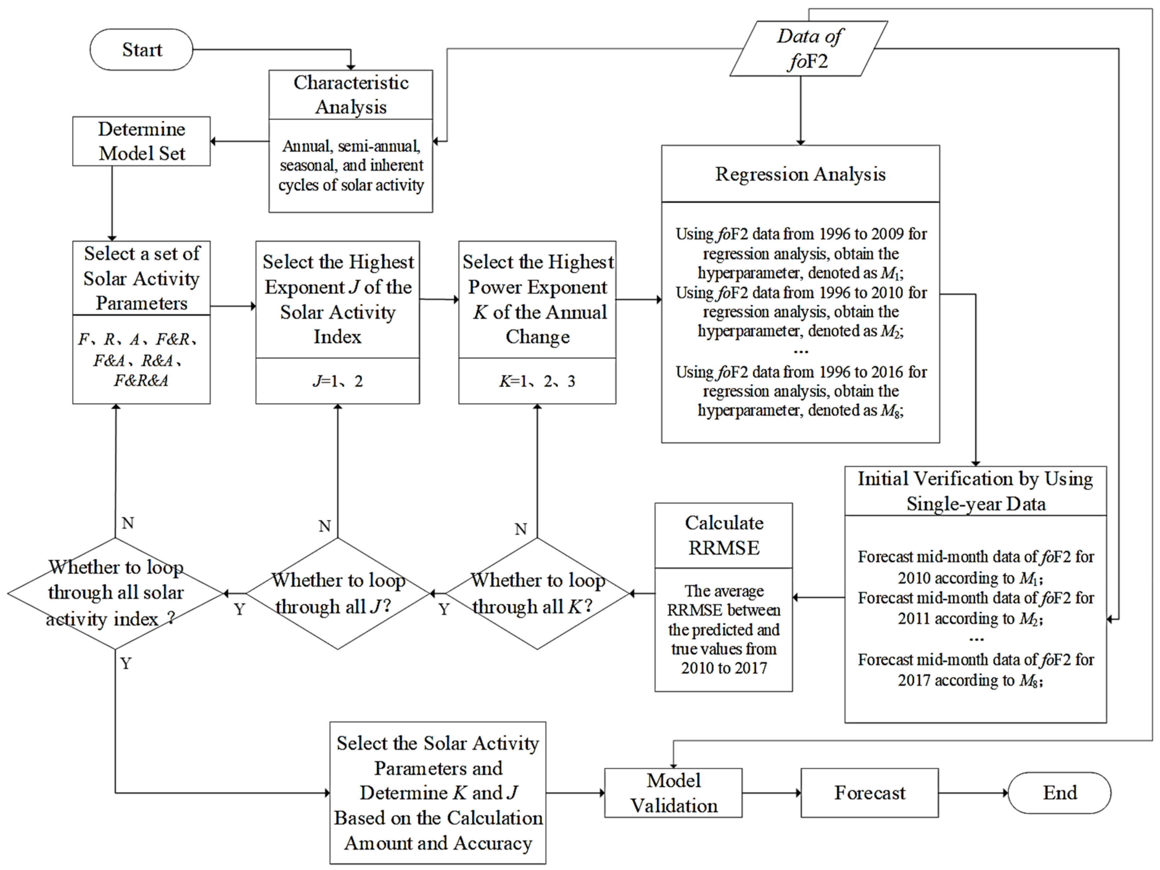
Figure 2 shows the modeling process using SML as follows:

(1)

Analyze the time variation characteristics of foF2 and determine the model set according to the annual, semi-annual, seasonal, and inherent cycle variation rules of solar activity;

(2)

Select a set of solar activity parameters, the highest exponent J of the solar activity index, and the highest exponent K of annual change;

(3)

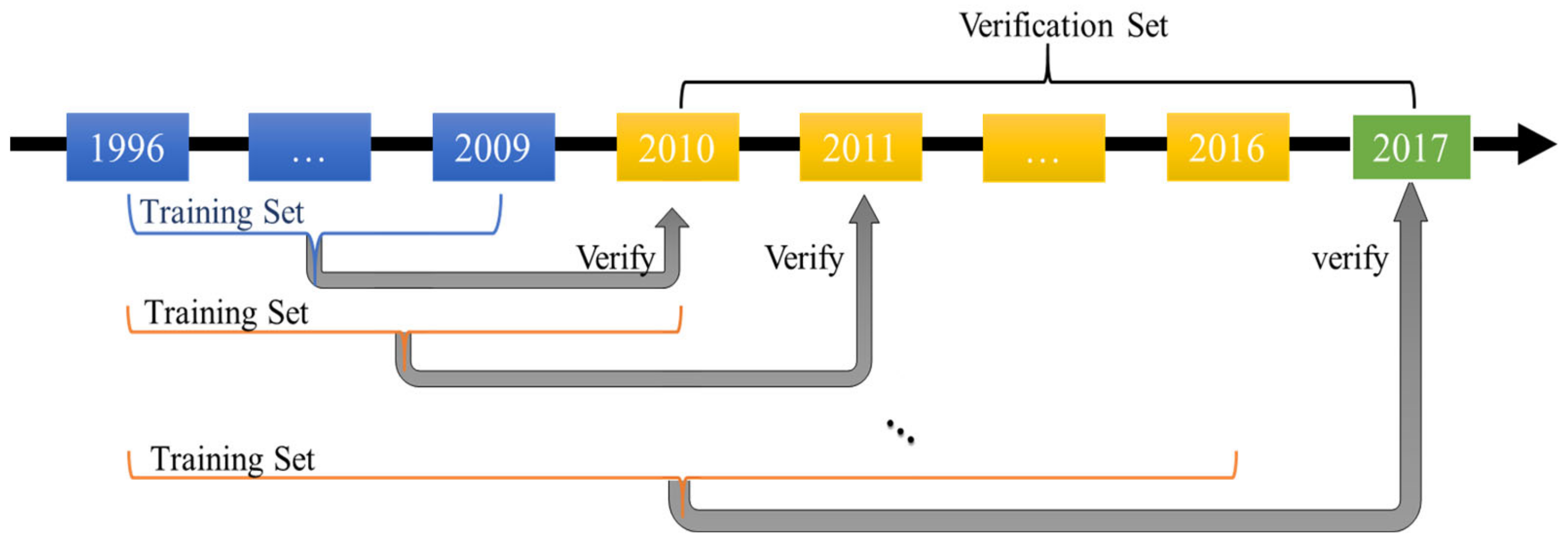
Conduct regression analysis based on the data of foF2 and conduct preliminary verification using single-year data. The specific process is as follows: First, use foF2 data from 1996 to 2009 for regression analysis, obtain the hyperparameter, denoted as M₁, and forecast mid-month data of foF2 for 2010 according to M₁. Secondly, using foF2 data from 1996 to 2010 for regression analysis, obtain the hyperparameter, denoted as M₂, and forecast mid-month data of foF2 for 2011 according to M₂, and so on, using foF2 data from 1996 to 2016 for regression analysis, obtaining the hyperparameter, denoted as M₈, and forecasting the mid-month data of foF2 for 2017 according to M₈;

(4)

Calculate and record the mean RRMSE between the predicted and actual median values of foF2 from 2010 to 2017;

(5)

Judge, in turn, whether K, J, and all solar activity index combinations have been traversed. If the traversal is complete, proceed to the next step; if not, proceed to the next round of traversal until the traversal is completed;

(6)

Select the solar activity parameters and determine K and J based on the calculation amount and accuracy;

(7)

Validate the model. The effectiveness and reliability of the model are proven by comparing it with the IRI-URSI, IRI-CCIR, and ARIM models.

3. Data Collection

3.1. Processing Data of foF2

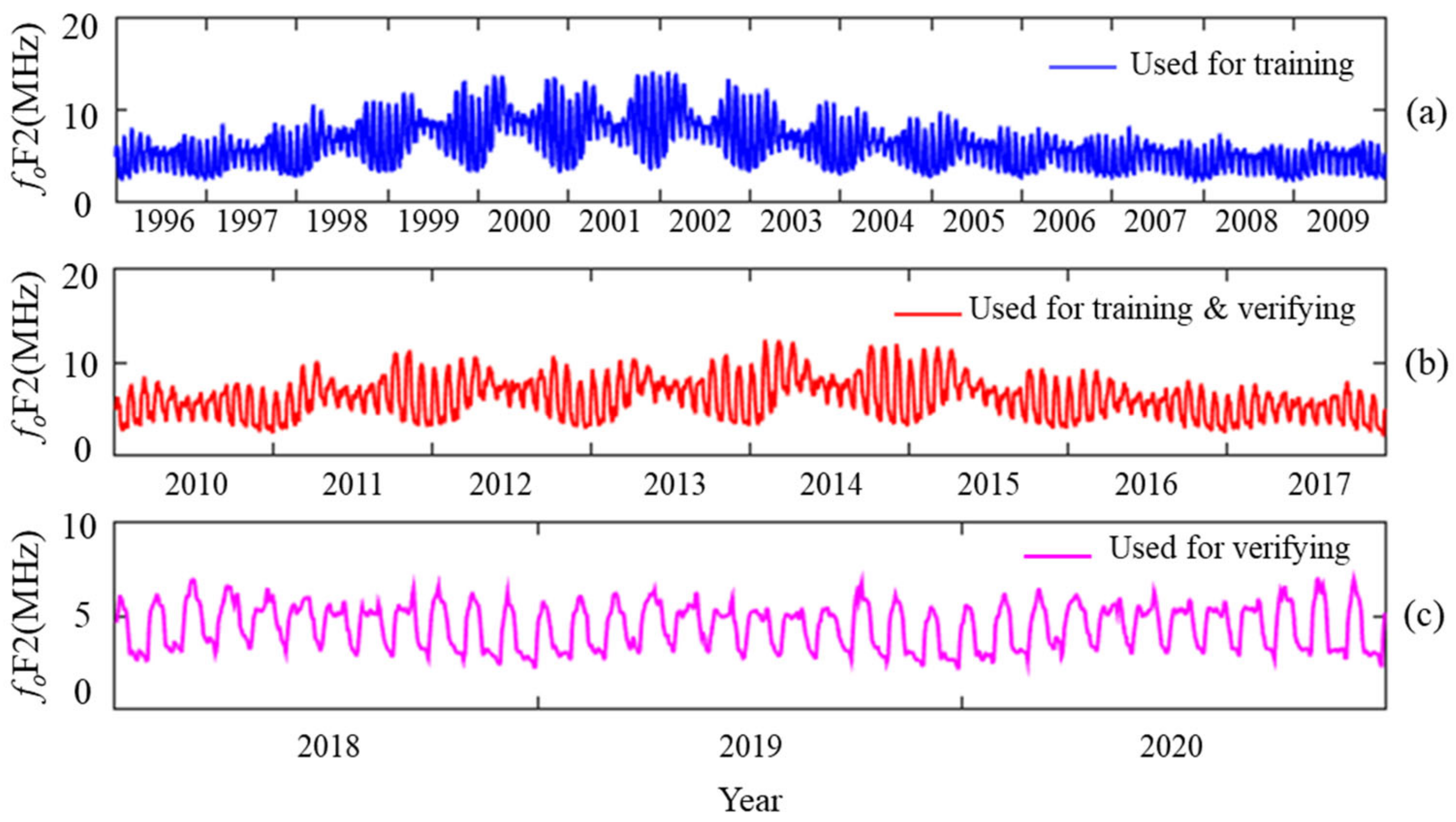
The foF2 data acquisition system is a general-purpose vertical-incidence sounding ionosonde [52], which has the advantages of easy installation, unattended operation, support for remote operation, and low maintenance costs [53]. The main functional performance parameters of the system include: (1) peak transmitting power—usually less than 5000 W; (2) rhe frequency range is wide. The coverage range is 2 MHz to 30 MHz; (3) sweep resolution: 25 kHz, 50 kHz, 75 kHz, or custom. As an example, foF2 data of Kokubunji station (35.7°N, 139.5°E) are used here for training and learning of the proposed model and parameters [54]. At the same time, we collected the corresponding solar activity parameters [55]. The selected observation station lies in the mid-latitude region and the data collected are shown in Figure 3. According to Figure 3, foF2 data collected from this station from 1996 to 2020 are complete, and the modeling selects a sampling interval of 1 h.

3.2. Deal with the Solar Activity Index

Usually, the solar activity index is used to describe the intensity of solar activity, described as follows: (1) the flux of solar radio waves with a wavelength of 10.7 cm (F10.7, which is labeled F), which is influenced by the corona and the upper atmosphere of the chromosphere [56]; (2) the number of sunspots (R), which is influenced by the photosphere and the lower chromosphere; (3) emission lines in the sun’s Lyman-alpha band (Lyman-α, labeled A) are the most vital lines in the ultraviolet band. Among them:

(1)

The solar 10.7 cm radio radiation flux is emitted from the outer chromosphere of the sun’s atmosphere and part of the bottom of the corona (inner corona). The unit of F10.7 is flux, and 1 sfu = 10⁻²² Wm⁻²Hz⁻¹ [55]. F10.7 is a solar activity index closely related to solar activity [57], and is widely used in solar and upper atmosphere empirical models, such as IRI [58,59] and NRLMSISI-00 [60]. Observations of F10.7 date back to 1947 and have a history of about 70 years, or about six solar cycles. This paper uses the 12-month sliding average of F, denoted as F₁₂. F10.7 data can be downloaded from the database of the National Oceanic and Atmospheric Administration (NOAA) [61];

(2)

Sunspot numbers are swirls of air caused by solid magnetic activity in the sun’s photosphere [62]. Since the first solar cycle in 1755, sunspot data have been observed for about 24 solar cycles. Because of its prolonged observation, the sunspot number R is the most widely used solar index. This paper uses the 12-month sliding average of R, denoted as R₁₂. The daily values provided by the SILSO database were considered [63];

(3)

Hydrogen emission at 121.6 nm represents the most robust single line in the ultraviolet band. It has been investigated in recent years by rockets, Atmospheric Explorer series satellites, the Solar Mesospheric Explorer, the Upper Atmosphere Research Satellite, Thermospheric Ionospheric Mesospheric Energy Dynamics, and the Solar Radiation and Climate Experiment mission [57]. In this paper, we use the 12-month sliding average of A, which is denoted as A₁₂. Detailed information about this composite dataset and free downloadable data are available at the website [64].

In the above, the formula for calculating the 12-month sliding average is as follows:

$$M_{12}=\frac{1}{12}[{\displaystyle \sum _{i=n-5}^{n+5}{\overline{M}}_i+\frac{1}{2}}({\overline{M}}_{n-6}+{\overline{M}}_{n+6})],$$

(1)

where $M$ is the solar activity index, $\overline{M}$ is the monthly average of the solar activity index, and n is the month of the required solar index.

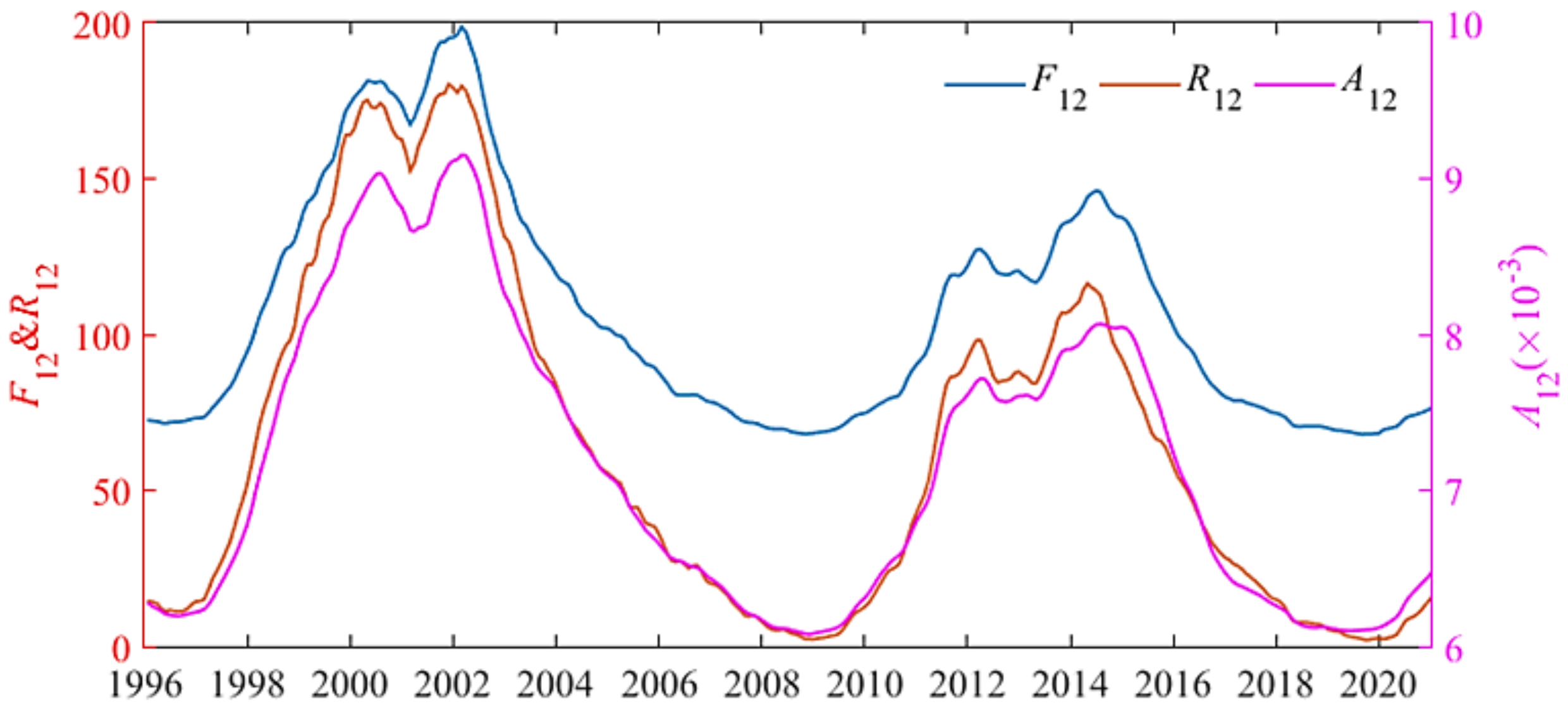
The changes in solar activity indexes F₁₂, R₁₂, and A₁₂ over time are shown in Figure 4. As can be seen, there are two complete cycles of solar activity between 1996 and 2020.

4. Model Construction

4.1. Data Analysis

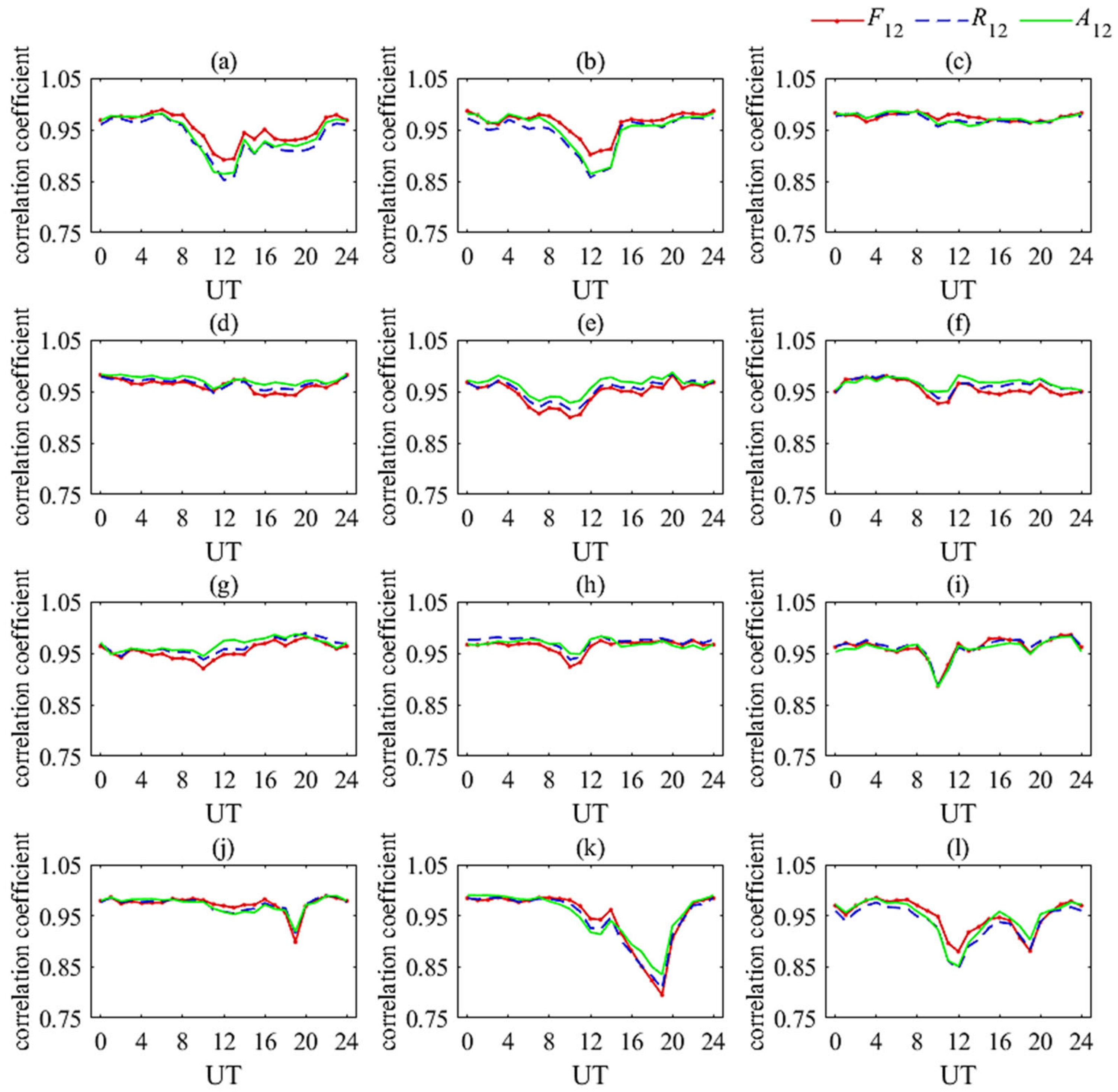
According to the data collected above, Figure 5 shows the correlation coefficients (CC) between the monthly median value of foF2 of Kokubunji station from 1996 to 2020 and the three types of solar activity index (F₁₂, R₁₂, and A₁₂) by month and hour. As shown in Figure 5, the values of the three groups’ CC are mostly between 0.8 and 1, indicating that the median value of foF2 significantly correlates with the three types of solar activity index. In addition, the variation trends of the three groups’ CC are similar, but there are differences in some minor details. Among the three groups of CC data, in November, when UT = 19, values are all the smallest, but specifically, they are 0.79, 0.81, and 0.83 respectively.

In summary, it is considered that foF2 is directly related to F₁₂, R₁₂, or A₁₂, but there are specific differences in different periods.

4.2. Model Set

According to the atmosphere–ionosphere–magnetosphere coupling mechanism [65,66,67] and the previous section’s analysis, this paper takes the correlation between foF2 and the above three types of solar activity indices [68] and the annual, semi-annual, seasonal, and more subtle changes of ionospheric characteristic parameters [1] into account. Therefore, the training model is selected for the given geographical coordinates and local time. The general formula for defining the harmonic mapping between foF2 and solar cycle variation parameters, year, season, and month is shown in Equation (2):

$$fo\mathrm{F}2(p,m)={\displaystyle \sum _{k=0}^K{\displaystyle \sum _{j=0}^J\left[{\gamma }_{k,j}{p}^j\cdot \cos (2\pi \mathrm{km}/12)+{\eta }_{k,j}{p}^j\cdot \sin (2\pi \mathrm{km}/12)\right]}},$$

(2)

where p represents F₁₂, R₁₂, or A₁₂.

Further, the above formula can be converted to Equation (3):

$$fo\mathrm{F}2(F_{12},R_{12},A_{12},m)=\underset{i=1}{\overset{3}{\cup |\cap }}{\displaystyle \sum _{j=0}^J{\displaystyle \sum _{k=0}^K[{\gamma }_{i,k,j}{p}_i{}^j\cdot \cos (2\pi \mathrm{km}/12)+}}{\eta }_{i,k,j}{p}_i{}^j\cdot \sin (2\pi \mathrm{km}/12)],$$

(3)

In Equations (2) and (3), m is an integer representing the month; in the trigonometric functions, the harmonic number k represents the periodic variation characteristics of year, half-year, season, and month. k = 1, 2, 3, and 4, and represents twelve months, six months, three months, and one month, respectively, where the denominator 12 represents the maximum value of the time cycle and corresponds to 12 months of a year. k = 0 represents a constant term. Considering that K = 4 is relative to K = 3, the increase in calculation amount does not significantly reduce the error [26], so we choose k = 1, 2, and 3 here. j represents the variation in the solar activity index, represented by functions of order 1, 2, 3, or higher. The highest harmonic frequency (K and J) can be determined by regression analysis. The coefficient is calculated from the observational data and the corresponding solar activity index.

4.3. Determined Parameters

Figure 6 shows that the model is established by dynamic enhanced prediction. First, the data set is divided into a complete training data set and a full verification data set. The complete training dataset includes foF2 data from 1996 to 2009, the first validation dataset includes foF2 data from 2010 to 2017, and the test dataset includes foF2 data from 2018 to 2020.

First, the data from 1996 to 2009 are used as training data, and the data from 2010 are used as initial validation data to obtain the prediction results of foF2 in 2010. Second, we used data of foF2 from 1996 to 2010 as training data and data from 2011 as initial validation data to obtain prediction results of foF2 in 2011, and so on, until the data from 1996 to 2016 are used as training data and the data from 2017 as validation data; thus, the prediction results of foF2 in 2017 are obtained. Finally, we calculate the RRMSE between the predicted foF2 and the real foF2 from 2010 to 2017. Then the final prediction model is selected from the model set based on the amount of calculation and RRMSE.

Among them, the calculation amount can be determined by Equation (4) according to Equation (3):

$$C{M}_s=c\cdot \left[\left(3J+K\right)f_{+}+4\left(J+1\right)f_{\times }+\left(J+1\right)f_2+\left(K+1\right)f_{\Delta }\right],$$

(4)

where c is the number of solar activity indices, f₊ represents the number of addition operations, f_× represents the number of multiplication operations, f₂ represents the number of square operations, and f_Δ represents the number of sine or cosine operations. If the four types of operation times are assumed to be equal, then Equation (4) can be simplified to the form shown in Equation (5):

$$C{M}_s=c\cdot \left(8J+2K+6\right)\cdot f,$$

(5)

where f represents f₊, f_×, f₂, and f_Δ.

It can be seen from Equation (5) that the calculated amount is proportional to the number of solar activity parameters, and the change with J is more drastic than that with K.

At the same time, the RRMSE is selected as the evaluation strategy and expressed as:

$$\mathrm{RRMSE}=\sqrt{\frac{1}{N}{\displaystyle \sum _{i=1}^N{\left(\frac{fo\mathrm{F}{2}_i^{\prime }-fo\mathrm{F}{2}_i}{fo\mathrm{F}{2}_i}\right)}^2}},$$

(6)

where $fo\mathrm{F}{2}_i^{\prime }$ is the prediction of the model, $fo\mathrm{F}{2}_i$ is the measured value, and N is the total data volume.

Figure 7 shows the radar diagram of the RRMSE and computation amounts for different modeling orders J and K obtained by SML. In the figure, 10, 20, 30, etc., can not only represent the amount of computation, but also the value of 4×RRMSE (%). The analysis found that:

(1)

When the value of J is the same, K = 2 has an increase compared with K = 1, but the RRMSE has a significant decrease; K = 3 has an increase compared with K = 2, but the RRMSE does not have a significant decrease;

(2)

When the values of J and K are the same, the calculation amount of a single solar activity parameter is less than that of multiple solar activity parameters. However, the RRMSE is similar to or even smaller than that obtained with multiple solar activity parameters;

(3)

Under the same conditions, the regression prediction effect using a single solar activity parameter R₁₂ is worse than that using F₁₂ or A₁₂.

According to the above analysis results, when J = 1, 2 and K = 1, 2, respectively, the calculation amounts required when using solar activity indices F and A for modeling prediction and the RRMSE are calculated. A comparison showed that the increased percentage of the calculation amount and the decreased percentage of the RRMSE when J = 1 and K = 1 were used for modeling.

Figure 7. Radar map of calculation amount and 4 × RRMSE(%) under different solar activity parameters J and K: (a) J = 1; (b) J = 2.

Figure 7. Radar map of calculation amount and 4 × RRMSE(%) under different solar activity parameters J and K: (a) J = 1; (b) J = 2.

As shown in Figure 8, J and K are both determined to be 2 by combining RRMSE values and considering engineering complexity.

According to the determined J = 2 and K = 2, the time regression prediction equation can be explicitly expressed as:

$$\begin{array}{cc}\hfill {\widehat{f}}_o\mathrm{F}2\left(F,m\right)& =\sum _{k=0}^2\sum _{j=0}^2\left[{\gamma }_{{}_{k,j}}{F}^j·cos\left(\frac{2\pi \mathrm{km}}{12}\right)\right.+\left.{\eta }_{{}_{k,j}}{F}^j·sin\left(\frac{2\pi \mathrm{km}}{12}\right)\right]\hfill \\ & =\left({\gamma }_{{}_{0,0}}+{\gamma }_{{}_{0,1}}F+{\gamma }_{{}_{0,2}}{F}^2\right)+\left({\gamma }_{{}_{1,0}}+{\gamma }_{{}_{1,1}}F+{\gamma }_{{}_{1,2}}{F}^2\right)·cos\left(\frac{2\pi \mathrm{m}}{12}\right)+\left({\gamma }_{{}_{2,0}}+{\gamma }_{{}_{2,1}}F+{\gamma }_{{}_{2,2}}{F}^2\right)·cos\left(\frac{2\pi \mathrm{m}}{6}\right)+\hfill \\ & \left({\eta }_{{}_{0,0}}+{\eta }_{{}_{0,1}}F+{\eta }_{{}_{0,2}}{F}^2\right)+\left({\eta }_{{}_{1,0}}+{\eta }_{{}_{1,1}}F+{\eta }_{{}_{1,2}}{F}^2\right)·sin\left(\frac{2\pi \mathrm{m}}{12}\right)+\left({\eta }_{{}_{2,0}}+{\eta }_{{}_{2,1}}F+{\eta }_{{}_{2,2}}{F}^2\right)·sin\left(\frac{2\pi \mathrm{m}}{6}\right)\hfill \end{array}$$

(7)

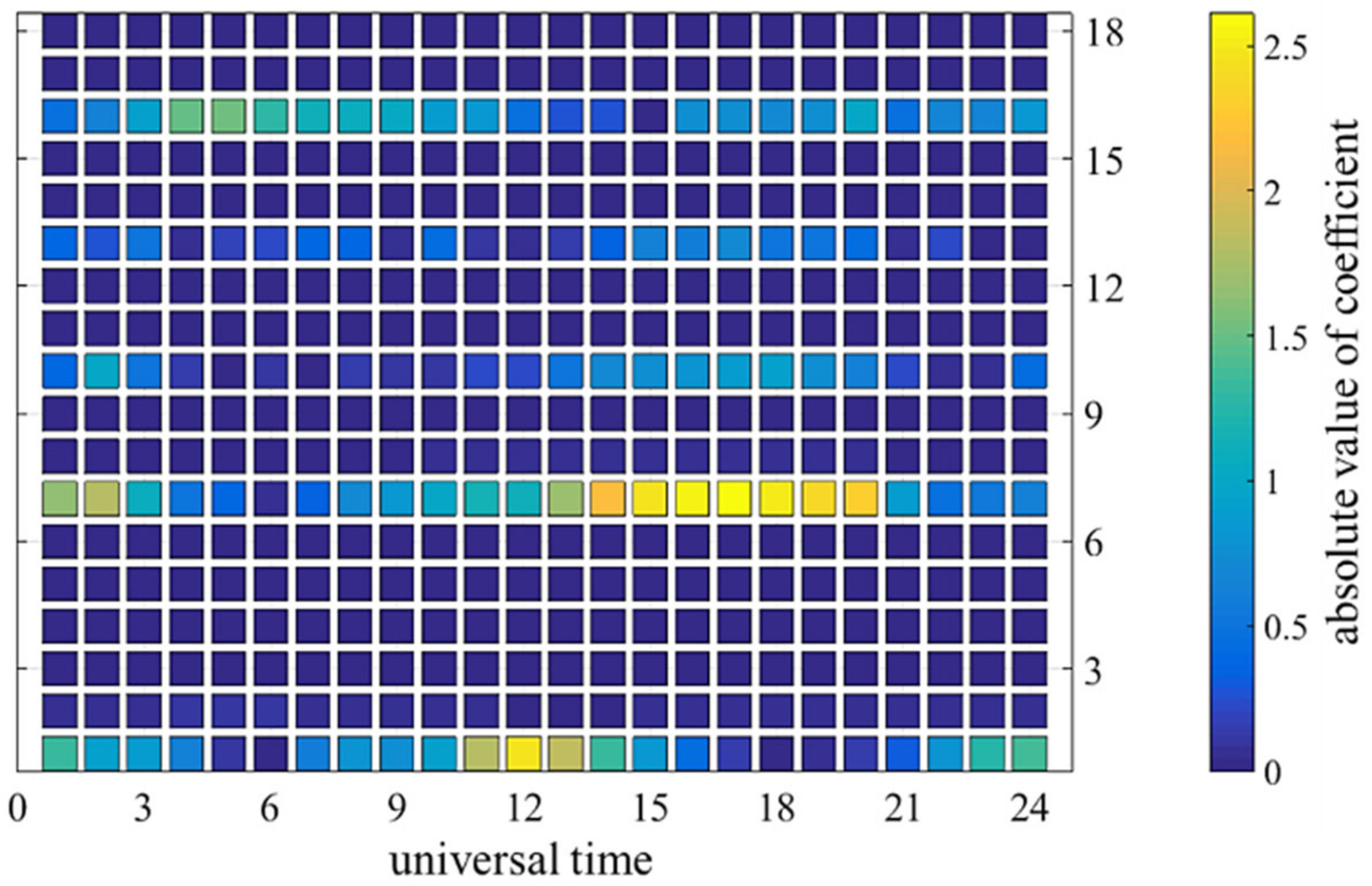
According to Equation (7), the observation data of Kokubunji station are used for LS regression analysis, and the corresponding η_k,j, γ_k,j, η′_k,j, and γ′_k,j of the station can be obtained. Figure 9 shows the distribution of coefficients γ_k,j and η_k,j using Kokubunji station in 2017 as an example. Coordinate marks 1~18 in the figure correspond to γ_0,0, γ_0,1, γ_0,2, η_0,0, η_0,1, η_0,2, γ_1,0, γ_1,1, γ_1,2, η_1,0, η_1,1, η_1,2, γ_2,0, γ_2,1, γ_2,2, η_2,0, η_2,1, and η_2,2 respectively.

5. Model Verification

To verify the predictive accuracy of the proposed model (identified as PROP), the predictive performance of the new model is compared with that of IRI-2016 [69] and ARFM [23]. The steps to obtain the prediction of foF2 from the PROP model are as follows:

(1)

According to Equation (7), the median data of foF2 from 1996 to 2017, 1996 to 2018, and 1996 to 2019 were used for regression analysis training, and we obtained the three corresponding groups of hyperparameters, denoted as M₉, M₁₀, and M₁₁;

(2)

According to M₉, M₁₀, and M₁₁, and according to F₁₂ of 2018, 2019, and 2020, the monthly median forecast of 2018, 2019, and 2020 is obtained by substituting Equation (7).

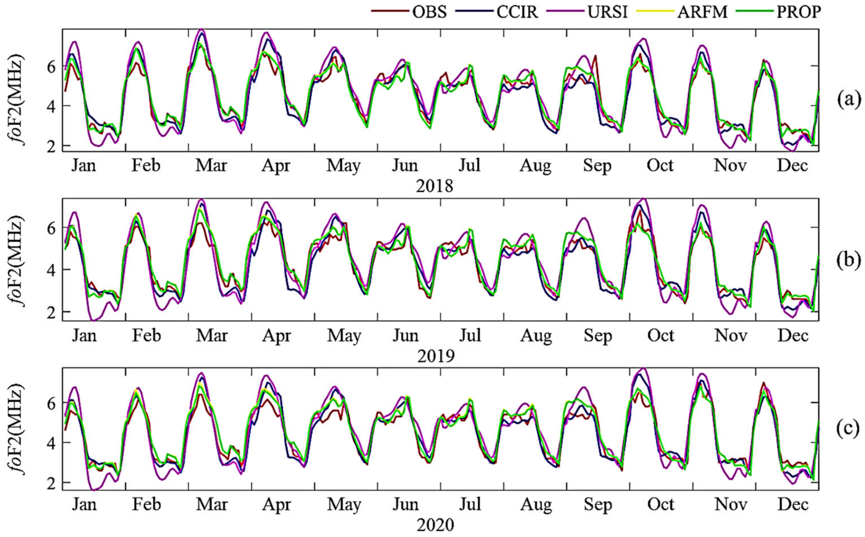
Figure 10 compares the predictions of the IRI model, ARFM model, PROP model, and the real monthly median value of foF2 from 2018 to 2020. The difference between the predictions of the IRI model and the real monthly median value of foF2 is significant. The predicted value of the ARFM and PROP models is close to the actual value of the monthly median value of foF2.

To further evaluate the models’ accuracy, the statistical mean value of MAE and RRMSE (Equation (6)) are calculated to statistically analyze the error between the median value of foF2 of the prediction model and the median value of the measured value. MAE is calculated by the following formula:

$$\mathrm{MAE}=\frac{1}{N}{\displaystyle \sum _i^N\left|fo{\mathrm{F}2}_{\mathrm{i}}^{\prime }-fo{\mathrm{F}2}_{\mathrm{i}}\right|},$$

(8)

where $fo\mathrm{F}{2}_i^{\prime }$ is the prediction of the model, $fo\mathrm{F}{2}_i$ is the measured value, and N is the total data volume.

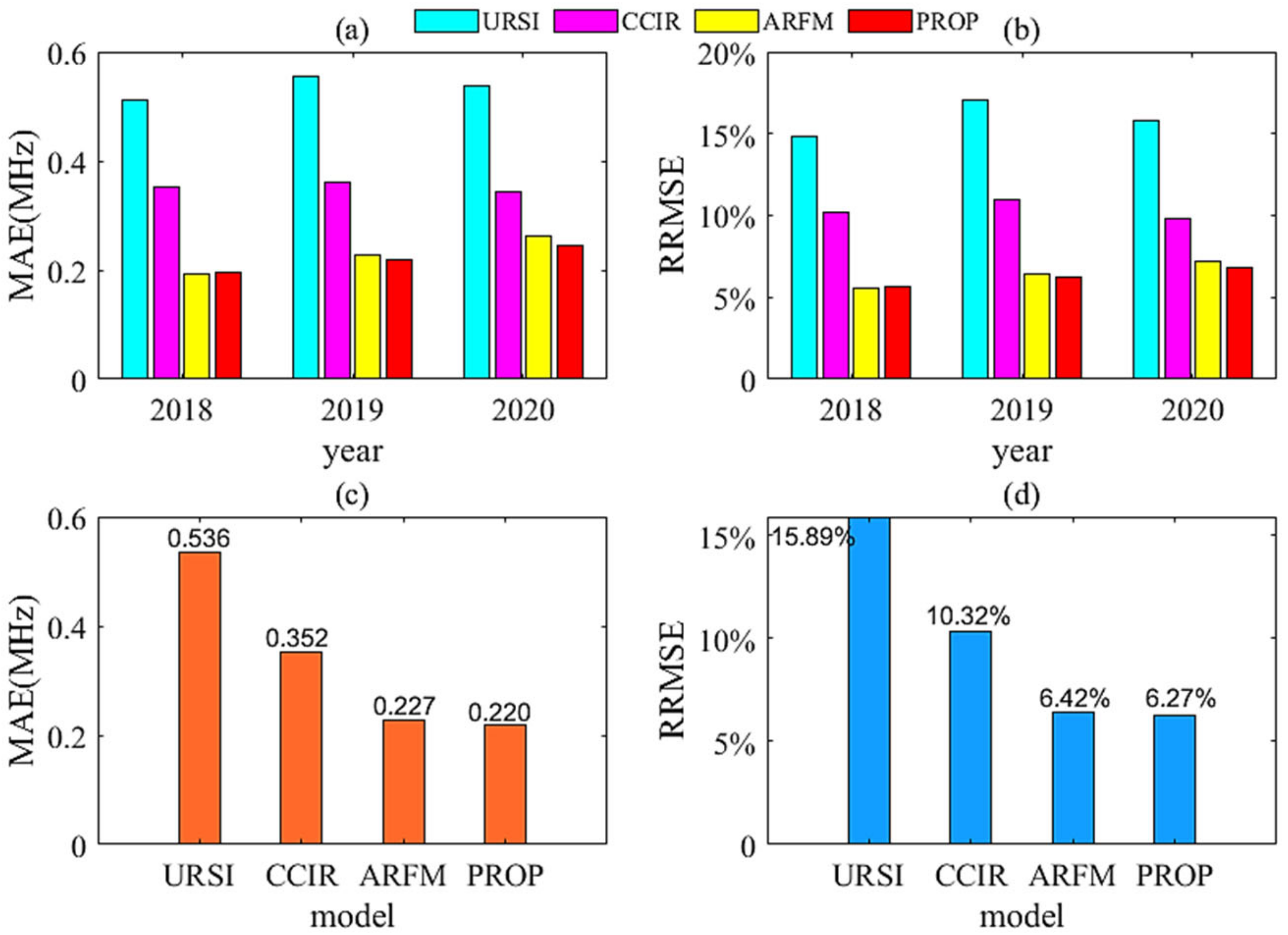
Figure 11 shows the foF2 statistical error diagram of the IRI-URSI, IRI-CCIR, ARFM, and PROP models. From 2018 to 2020, the MAE and RRMSE between the predictions of the IRI model and the observations are more significant than those of the PROP model. However, in 2018, the MAE and RRMSE between the predicted value and the actual value of the ARFM model are slightly smaller than those of the PROP model. Nevertheless, considering the average of three years, the PROP model still has some advantages.

Specifically, the MAEs corresponding to the IRI-URSI model, IRI-CCIR model, ARFM model, and PROP model are 0.536 MHz, 0.352 MHz, 0.227 MHz, and 0.220 MHz, respectively. Compared with the IRI-URSI, IRI-CCIR, and ARFM models, the statistical average MAE corresponding to foF2 decreased by 0.316 MHz, 0.132 MHz, and 0.007 MHz, respectively. The RRMSEs corresponding to the IRI-URSI model, IRI-CCIR model, ARFM model, and PROP model are 15.89%, 10.32%, 6.42%, and 6.27%, respectively. Compared with the IRI-URSI, IRI-CCIR, and ARFM models, the statistical average RRMSE corresponding to foF2 decreased by 9.62%, 4.05%, and 0.15%, respectively. The reconstruction model PROP in Kokubunji station has higher precision than the IRI and ARFM models. In other words, the PROP model in this station has realized improvements against the IRI and ARFM models.

6. Conclusions

This paper uses an ML method to propose an interpretable dynamic predictive annual regression model of the ionospheric foF2 median value. The model’s main features are as follows: (1) using a dynamic data-updating method for dynamic training prediction; (2) using only one solar activity parameter can achieve high precision prediction and reduce engineering complexity. Compared with the IRI-2016 model and the ARFM model, this model still has some advantages in the prediction performance of foF2 parameters of Kokubunji station. In addition, a goal of future work is to compare the proposed model with other methods such as LSTM and Bi-LSTM. Future research expects to extend the model’s applicability to a broader range of stations, regions, and even globally. In addition, this modeling method can be used to predict other ionospheric parameters, such as total electron content and peak height. This method can also be used for natural hazard and space weather monitoring.

References

1. Qian, L.Y.; Burns, A.G.; Solomon, S.C.; Wang, W.B. Annual/semiannual variation of the ionosphere. Geophys. Res. Lett. 2013, 40, 1928–1933. [Google Scholar] [CrossRef]
2. Wang, J.; Yang, C.; An, W. Regional Refined Long-term Predictions Method of Usable Frequency for HF Communication Based on Machine Learning over Asia. IEEE Trans. Antennas Propag. 2022, 70, 4040–4055. [Google Scholar] [CrossRef]
3. Fagre, M.; Zossi, B.S.; Chum, J.; Yigit, E.; Elias, A.G. Ionospheric high frequency wave propagation using different IRI hmF2 and foF2 models. J. Atmos. Sol.-Terr. Phys. 2019, 196, 105141. [Google Scholar] [CrossRef]
4. Swamy, K.C.T.; Sarma, A.D.; Srinivas, V.S.; Kumar, P.N.; Rao, P.V.D.S. Accuracy evaluation of estimated ionospheric delay of GPS signals based on Klobuchar and IRI-2007 models in low latitude region. IEEE Geosci. Remote Sens. Lett. 2013, 10, 1557–1561. [Google Scholar] [CrossRef]
5. Erdogan, E.; Seitz, F. High-Resolution Ionosphere Corrections for Single-Frequency Positioning. Remote Sens. 2021, 13, 12. [Google Scholar]
6. Wang, J.; Yang, C.; Yan, C. Study on digital twin channel for the B5G and 6G communication. Radio Sci. 2021, 36, 340–348. [Google Scholar]
7. Thayaparan, T.; Marchioni, J.; Kelsall, A.; Riddolls, R. Improved Frequency Monitoring System for Sky-Wave Over-the-Horizon Radar in Canada. IEEE Geosci. Remote Sens. Lett. 2020, 17, 606–610. [Google Scholar] [CrossRef]
8. Ikuta, R.; Oba, R.; Kiguchi, D.; Hisada, T. Reanalysis of the ionospheric total electron content anomalies around the 2011 Tohoku-Oki and 2016 Kumamoto earthquakes: Lack of a clear precursor of large earthquakes. J. Geophys. Res. Space Phys. 2021, 126, e2021JA029376. [Google Scholar] [CrossRef]
9. Santis, A.D.; Perrone, L.; Calcara, M.; Campuzano, S.A.; Cianchini, G.; D’Arcangelo, S.; Mauro, D.D.; Marchetti, D.; Nardi, A.; Orlando, M.; et al. A comprehensive multiparametric and multilayer approach to study the preparation phase of large earthquakes from ground to space: The case study of the June 15 2019, M7.2 Kermadec Islands (New Zealand) earthquake. Remote Sens. Environ. 2022, 283, 113325. [Google Scholar] [CrossRef]
10. Wang, J.; Shi, Y.; Yang, C. Investigation of Two Prediction Models of Maximum Usable Frequency for HF Communication Based on Oblique- and Vertical-Incidence Sounding Data. Atmosphere 2022, 13, 1122. [Google Scholar] [CrossRef]
11. Bilitza, D. IRI the international standard for the ionosphere. Adv. Radio Sci. 2018, 53, 1–11. [Google Scholar] [CrossRef] [Green Version]
12. Bilitza, D.; Mckinnell, L.A.; Reinisch, B.; Rowell, T.F. The international reference ionosphere today and in the future. J. Geod. 2011, 85, 909–920. [Google Scholar] [CrossRef]
13. Bilitza, D.; Altadill, D.; Truhlik, V.; Shubin, V.; Galkin, I.; Reinisch, B.; Huang, X. International reference ionosphere 2016: From ionospheric climate to real-time weather predictions. Space Weather 2017, 15, 418–429. [Google Scholar] [CrossRef]
14. Wang, J.; Shi, Y.; Yang, C. An Overview and Prospects of Operational Frequency Selecting Techniques for HF Radio Communication. Adv. Space Res. 2022, 69, 2989–2999. [Google Scholar] [CrossRef]
15. Sun, X.R. A method of predicting the ionospheric Flayer in the Asia Oceania region. J. China Inst. Commun. 1987, 8, 153–156. [Google Scholar]
16. Cao, H.; Sun, X.R. A new method of predicting the ionospheric F2 layer in the Asia Oceania region. Space Sci. 2009, 29, 502–507. [Google Scholar] [CrossRef]
17. Bhuyan, P.K.; Chamua, M. An empirical model of electron temperature in the Indian topside ionosphere for solar minimum based on SROSS C2 RPA data. Adv. Space Res. 2006, 37, 897–902. [Google Scholar] [CrossRef]
18. Brunini, C.; Meza, A.; Gende, M.; Azpilicueta, F. South American regional ionospheric maps computed by GESA: A pilot service in the framework of SIRGAS. Adv. Space Res. 2007, 42, 737–744. [Google Scholar] [CrossRef]
19. An, J.C.; Ning, X.J.; Wang, Z.M.; Zhang, X. Antarctic ionospheric prediction based on spherical cap harmonic analysis and time series analysis. Wuhan Daxue Xuebao 2015, 40, 677–681. [Google Scholar]
20. Themens, D.R.; Jayachandran, P.T.; Galkin, I.; Hall, C. The Empirical Canadian High Arctic Ionospheric Model (E-CHAIM): NmF2 and hmF2. J. Geophys. Res. Space Phys. 2017, 122, 9015–9031. [Google Scholar] [CrossRef]
21. Perna, L.; Pezzopane, M.; Pietrella, M.; Zolesi, B.; Cander, L.R. An updating of the SIRM model. Adv. Space Res. 2017, 60, 1249–1259. [Google Scholar] [CrossRef]
22. Song, R.; Zhang, X.M.; Zhou, C.; Liu, J.; He, J.H. Predicting TEC in China based on the neural networks optimized by genetic algorithm. Adv. Space Res. 2018, 62, 745–759. [Google Scholar] [CrossRef]
23. Wang, J.; Ma, J.G.; Huang, X.D.; Bai, H.M.; Chen, Q.; Cheng, H. Modeling of the Ionospheric Critical Frequency of the F2 layer over Asia based on Modified Temporal-Spatial Reconstruction. Radio Sci. 2019, 54, 680–691. [Google Scholar] [CrossRef]
24. Okoh, D.; Seemala, G.; Rabiu, B.; Habarulema, J.B.; Jin, S.; Shiokawa, K.; Otsuka, Y.; Aggarwal, M.; Uwamahoro, J.; Mungufeni, P.; et al. A neural network-based ionospheric model over Africa from Constellation Observing System for Meteorology, Ionosphere, and Climate and Ground Global Positioning System observations. J. Geophys. Res. Space Phys. 2019, 124, 10512–10532. [Google Scholar] [CrossRef]
25. Wang, J.; Bai, H.; Huang, X.; Cao, Y.; Chen, Q.; Ma, J. Simplified Regional Prediction Model of Long-Term Trend for Critical Frequency of Ionospheric F2 Region over East Asia. Appl. Sci. 2019, 9, 3219. [Google Scholar] [CrossRef] [Green Version]
26. Wang, J.; Feng, F.; Bai, H.M.; Cao, Y.B.; Chen, Q.; Ma, J.G. A regional model for the prediction of M(3000)F2 over East Asia. Adv. Space Res. 2020, 65, 2036–2051. [Google Scholar] [CrossRef]
27. Jeong, S.-H.; Lee, W.K.; Jang, S.; Kil, H.; Kim, J.-H.; Kwak, Y.-S.; Kim, Y.H.; Hong, J.; Choi, B.K. Reconstruction of the Regional Total Electron Content Maps Over the Korean Peninsula Using Deep Convolutional Generative Adversarial Network and Poisson Blending. Space Weather 2022, 20, e2022SW003131. [Google Scholar] [CrossRef]
28. Abuelezz, O.A.; Mahrous, A.M.; Cilliers, P.J.; Fleury, R.; Youssef, M.; Nedal, M.; Yassen, A.M. Neural network prediction of the topside electron content over the Euro-African sector derived from Swarm-A measurements. Adv. Space Res. 2021, 67, 1191–1209. [Google Scholar] [CrossRef]
29. Kim, J.-H.; Kwak, Y.S.; Kim, Y.; Moon, S.-I.; Jeong, S.-H.; Yun, J. Potential of Regional Ionosphere Prediction Using a Long Short-Term Memory Deep-Learning Algorithm Specialized for Geomagnetic Storm Period. Space Weather 2021, 19, e2021SW002741. [Google Scholar] [CrossRef]
30. Ameen, M.A.; Tahir, A.; Talha, M.; Khursheed, H.; Siddiqui, I.A.; Iqbal, S.T.; Gul, B. Modelling of foF2 using artificial neural network over Equatorial Ionization Anomaly (EIA) region stations. Adv. Space Res. 2022. [Google Scholar] [CrossRef]
31. Adebesin, B.O.; Adeniyi, J.O.; Afolabi, P.A.; Ikubanni, S.O.; Adebiyi, S.J. Modelling M(3000)F2 at an African Equatorial Location for Better IRI-Model Prediction. Radio Science 2022, 57, e2021RS007311. [Google Scholar] [CrossRef]
32. Sivavaraprasad, G.; Mallika, I.L.; Sivakrishna, K.; Ratnam, D.V. A novel hybrid Machine learning model to forecast ionospheric TEC over Low-latitude GNSS stations. Adv. Space Res. 2022, 69, 1366–1379. [Google Scholar] [CrossRef]
33. Moon, S.; Kim, Y.H.; Kim, J.H.; Kwak, Y.S.; Yoon, J.Y. Forecasting the ionospheric F2 parameters over Jeju Station (33.43◦N, 126.30◦E) by using long short-term memory. J. Korean Phys. Soc. 2020, 77, 11. [Google Scholar] [CrossRef]
34. Inyurt, S.; Kashani, M.H.; Sekertekin, A. Ionospheric TEC forecasting using Gaussian process regression (GPR) and multiple linear regression (MLR) in Turkey. Astrophys. Space Sci. 2020, 365, 99. [Google Scholar] [CrossRef]
35. Bai, H.M.; Feng, F.; Wang, J.; Wu, T.S. Modeling M(3000)F2 based on Extreme Learning Machine. Adv. Space Res. 2020, 65, 107–114. [Google Scholar]
36. Zhao, J.; Li, X.J.; Liu, Y.; Wang, X.; Zhou, C. Ionospheric foF2 disturbance forecast using neural network improved by a genetic algorithm. Adv. Space Res. 2019, 63, 4003–4014. [Google Scholar] [CrossRef]
37. Ameen, M.A.; Jabbar, M.A.; Murtaza, G.; Chishtie, F.; Xu, T.; Zhen, W.M.; Atiq, M.; Ali, M.S. Single station modelling and comparison with ionosonde foF2 over Karachi from 1983–2007. Adv. Space Res. 2019, 64, 2104–2113. [Google Scholar] [CrossRef]
38. Tshisaphungo, M.; Habarulema, J.B.; McKinnell, L.-A. Modeling ionospheric foF2 response during geomagnetic storms using neural network and linear regression techniques. Adv. Space Res. 2018, 61, 2891–2903. [Google Scholar] [CrossRef]
39. Wang, J.; Liu, Y.; Xu, C. The Progress Review and Future Preview of Typical Ionospheric Models. In Proceedings of the International Symposium on Antennas, Propagation and EM Theory, Zhuhai, China, 30 November 2021. [Google Scholar]
40. Bai, H.M.; Fu, H.P.; Wang, J.; Ma, K.X.; Wu, T.S.; Ma, J.G. A prediction model of ionospheric foF2 based on extreme learning machine. Radio Sci. 2018, 53, 1292–1301. [Google Scholar] [CrossRef]
41. Fan, J.Q.; Liu, C.; Lv, Y.J.; Han, J.; Wang, J. A Short-Term Forecast Model of foF2 Based on Elman Neural Network. Appl. Sci. 2019, 9, 2782. [Google Scholar]
42. Rao, T.V.; Sridhar, M.; Ratnam, D.V.; Harsha, P.B.S.; Srivani, I. A Bidirectional Long Short-Term Memory-Based Ionospheric foF2 and hmF2 Models for a Single Station in the Low Latitude Region. IEEE Geosci Remote Sens. Lett. 2022, 19, 8005405. [Google Scholar] [CrossRef]
43. Bi, C.; Ren, P.; Yin, T.; Zhang, Y.; Li, B.; Xiang, Z. An Informer Architecture-Based Ionospheric foF2 Model in the Middle Latitude Region. IEEE Geosci Remote Sens. Lett. 2022, 19, 1005305. [Google Scholar] [CrossRef]
44. Tsai, T.C.; Jhuang, H.K.; Ho, Y.Y.; Lee, L.C.; Su, W.C.; Hung, S.L.; Lee, K.H.; Fu, C.C.; Lin, H.C.; Kuo, C.L. Deep learning of detecting ionospheric precursors associated with M ≥ 6.0 earthquakes in Taiwan. Earth Space Sci. 2022, 9, e2022EA002289. [Google Scholar] [CrossRef]
45. Akhoondzadeh, M.; De Santis, A.; Marchetti, D.; Wang, T. Developing a Deep Learning-Based Detector of Magnetic, Ne, Te and TEC Anomalies from Swarm Satellites: The Case of Mw 7.1 2021 Japan Earthquake. Remote Sens. 2022, 14, 1582. [Google Scholar] [CrossRef]
46. Georgios, B.; Sigiava, A.-G.; Constantinos, P.; Ioannis, A.; Anastasios, A.; Roger, H. A machine learning approach for automated ULF wave recognition. J. Space Weather Space Clim. 2019, 9, A13. [Google Scholar]
47. Aa, E.; Zhang, D.; Xiao, Z.; Hao, Y.-Q.; Ridley, A.J.; Moldwin, M. Modeling ionospheric foF2 by using empirical orthogonal function analysis. Ann. Geophys. 2011, 29, 1501–1515. [Google Scholar]
48. Zhang, M.L.; Liu, C.; Wan, W.; Liu, L.; Ning, B. A global model of the ionospheric F2 peak height based on EOF analysis. Ann. Geophys. 2009, 27, 3203–3212. [Google Scholar] [CrossRef] [Green Version]
49. Oyeyemi, E.O.; Mckinnell, L.A. A new global F2 peak electron density model for the International Reference Ionosphere (IRI). Adv. Space Res. 2008, 42, 645–658. [Google Scholar] [CrossRef]
50. Fokoue, E. Model Selection for Optimal Prediction in Statistical Machine Learning. N. Am. Math. Soc. 2020, 67, 2. [Google Scholar] [CrossRef]
51. Santis, D. A Multiparametric Approach to Study the Preparation Phase of the 2019 M7.1 Ridgecrest (California, United States) Earthquake. Front. Earth Sci. 2020, 8, 540398. [Google Scholar] [CrossRef]
52. Bibl, K. Sixty years of ionospheric measurements and studies. Advances in Radio Science 2004, 2, 265–268. [Google Scholar] [CrossRef] [Green Version]
53. Lan, J.P.; Ning, B.Q.; Zhu, Z.P.; Hu, L.H.; Sun, W.J.; Li, G.Z. Development of agile digital ionosonde and its preliminary observation. Space Sci. 2019, 39, 167–177. [Google Scholar]
54. Ionosonde Data in JAPAN. Available online: https://wdc.nict.go.jp/IONO/HP2009/ISDJ/index-E.html (accessed on 3 November 2022).
55. Tapping, K.F. The 10.7cm solar radio flux (F10.7). Space Weather 2013, 11, 394–406. [Google Scholar] [CrossRef]
56. Afraimovich, E.L.; Astafyeva, E.I.; Oinats, A.V.; Yasukevich, Y.V.; Zhivetiev, I.V. Global electron content: A new conception to track solar activity. Ann. Geophys. 2008, 26, 335–344. [Google Scholar] [CrossRef] [Green Version]
57. Solomon, S.C.; Qian, L.; Burns, A.G. The anomalous ionosphere between solar cycles 23 and 24. Geophys. Res. Space Phys. 2013, 18, 6524–6535. [Google Scholar] [CrossRef]
58. Bilitza, D. International Reference Ionosphere, 3rd ed.; World Data Center A for Rockets and Satellites: Greenbelt, MA, USA, 1990. [Google Scholar]
59. Bilitza, D.; Altadill, D.; Zhang, Y.; Mertens, C.; Truhlik, V.; Richards, P.; McKinnell, L.A.; Reinisch, B. The International Reference Ionosphere 2012—A model of international collaboration. J. Space Weather Space Clim. 2014, 4, A07. [Google Scholar] [CrossRef]
60. Picone, J.M.; Hedin, A.E.; Drob, D.P.; Aikin, A.C. NRLMSISE-00 empirical model of the atmosphere: Statistical comparisons and scientific issues. J. Geophys. 2002, 107, 1–16. [Google Scholar] [CrossRef]
61. National Oceanic and Atmospheric Administration (NOAA). Available online: https://www.ngdc.noaa.gov/stp/space-weather/solar-data/ (accessed on 28 October 2022).
62. Sun, W. Study on Regional Ionospheric Characteristics Based on Ground-Based GPS and Occultation Technology; Wuhan University: Wuhan, China, 2015. [Google Scholar]
63. Sunspot Number. Available online: https://www.sidc.be/silso/datafiles (accessed on 28 October 2022).
64. Data of Hydrogen Emission at 121.6 nm. Available online: https://lasp.colorado.edu/lisird/composite_timeseries.html (accessed on 27 April 2022).
65. Editors, D.; Ouzounov, S.; Pulinets, K.; Hattori, T.P. Pre-Earthquake Processes: A Multidisciplinary Approach to Earthquake Prediction Studies; AGU & Wiley: Bristol, UK, 2018; pp. 79–99. [Google Scholar]
66. Santis, A.D.; Balasis, G.; Pavón-Carrasco, F.G.; Cianchini, G.; Mandea, M. Potential earthquake precursory pattern from space: The 2015 Nepal event as seen by magnetic Swarm satellites. Earth Planet. Sci. Lett. 2017, 461, 119–126. [Google Scholar] [CrossRef] [Green Version]
67. Ouzounov, D.; Pulinets, S.; Davidenko, D.; Rozhnoi, A.; Solovieva, M.; Fedun, V.; Dwivedi, B.N.; Rybin, A.; Kafatos, M.; Taylor, P. Transient Effects in Atmosphere and Ionosphere Preceding the 2015 M7.8 and M7.3 Gorkha–Nepal Earthquakes. Front. Earth Sci. 2021, 9, 757358. [Google Scholar] [CrossRef]
68. Zhang, X.; Le, G.; Zhang, Y. Phase relationship between the relative sunspot number and solar 10.7 cm flux. Chin. Sci. Bull. 2012, 57, 2078–2082. [Google Scholar] [CrossRef] [Green Version]
69. International Reference Ionosphere. Available online: http://IRImodel.org/IRI-2016 (accessed on 18 April 2022).
Figure 1. Three elements needed for modeling and four problems needed to be solved based on SML.
Remotesensing 15 01256 g001
Figure 2. Flow chart of long-term dynamic prediction model of foF2 based on SML.
Remotesensing 15 01256 g002
Figure 3. The data of foF2 of Kokubunji station: (a) used for training; (b) used for training and verifying; and (c) used for verifying.
Remotesensing 15 01256 g003
Figure 4. Figure of solar activity indexes over time.
Remotesensing 15 01256 g004
Figure 5. The correlation coefficients between the monthly median value of foF2 and solar activity indices by month: (a) Jan; (b) Feb; (c) Mar; (d) Apr; (e) May; (f) Jun; (g) Jul; (h) Aug; (i) Sept; (j) Oct; (k) Nov; (l) Dec.
Remotesensing 15 01256 g005
Figure 6. Schematic diagram of the dynamic enhanced prediction model.
Remotesensing 15 01256 g006
Figure 8. Schematic diagram of calculated increase percentage and RRMSE decrease percentage under different solar activity parameters and J and K conditions.
Remotesensing 15 01256 g008
Figure 9. Function reconstruction parameters.
Remotesensing 15 01256 g009
Figure 10. Comparison of IRI, ARFM, and reconstructed model with real value of foF2: (a) year of 2018; (b) year of 2019; (c) year of 2020.
Remotesensing 15 01256 g010
Figure 11. Statistical results of MAE and RRMSE between the predicted value and the real value of IRI, ARFM, and PROP models: (a) MAE of each year; (b) RRMSE of each year; (c) MAE of all years; (d) RRMSE of all years.
Remotesensing 15 01256 g011
Disclaimer/Publisher’s Note: The statements, opinions and data contained in all publications are solely those of the individual author(s) and contributor(s) and not of MDPI and/or the editor(s). MDPI and/or the editor(s) disclaim responsibility for any injury to people or property resulting from any ideas, methods, instructions or products referred to in the content.