Article

Statistical Analysis of SF Occurrence in Middle and Low Latitudes Using Bayesian Network Automatic Identification

1
China Research Institute of Radiowave Propagation (CRIRP), Qingdao 266107, China
2
Department of Space Physics, School of Electronic Information, Wuhan University, Wuhan 430072, China
3
National Time Service Center, Chinese Academy of Sciences, Beijing 100045, China
4
School of Artificial Intelligence, Hubei University, Wuhan 430061, China
*
Author to whom correspondence should be addressed.
Remote Sens. 2023, 15(4), 1108; https://doi.org/10.3390/rs15041108
Submission received: 11 January 2023 / Revised: 15 February 2023 / Accepted: 15 February 2023 / Published: 17 February 2023
(This article belongs to the Special Issue Ionosphere Monitoring with Remote Sensing II)

Abstract

:
Spread-F (SF) is one of the most important types of the ionospheric irregularities as it causes ionospheric scintillation which can severely affect the performance and reliability of communication, navigation, and radar systems. The ionosonde provides the most effective and economical way to study the ionosphere and SF. However, the manual identification of SF from an ionogram is boring and hard work. To automatically identify SF on the ionogram and extend the study of SF into the middle and low latitudes of East Asia, this paper presents a statistical analysis of SF in this region, based on the naïve Bayesian classifier. The results showed that the accuracy of automatic identification reached up to 97% on both the validation datasets and test datasets composed of Mohe, I-Cheon, Jeju, Wuhan, and Sanya ionograms, suggesting that it is a promising way to automatically identify SF on ionograms. Based on the classification results, the statistical analysis shows that SF has a complicated morphology in the middle and low latitudes of East Asia. Specifically, there is a peak of occurrence of SF in the summer in I-Cheon, Jeju, Sanya, and Wuhan; however, the Mohe station has the highest occurrence rate of SF in December. The different seasonal variations of SF might be due to the different geographic local conditions, such as the inland-coastal differences and formation mechanism differences at these latitudes. Moreover, SF occurs more easily in the post-midnight hours when compared with the pre-midnight period in these stations, which is consistent with the previous results. Furthermore, this paper extracts the frequency SF (FSF) index and range SF (RSF) index to characterize the features of SF. The results shows that the most intense FSF/RSF appeared in the height range of 220–300 km/1–7 MHz in these stations, although there are different magnitude extensions on different season in these regions. In particular, strong spread-F (SSF) reached its maximum at the equinox at Sanya, confirming the frequent SSF occurrence at the equinox at the equator and low latitudes. These results would be helpful for understanding the characteristics of SF in East Asia.

1. Introduction

Spread-F (SF) is one of the most prominent manifestations of ionospheric plasma instability, which is able to influence the performance and reliability of electronic systems, such as satellite, radar, navigation, and communication systems [1,2]. Therefore, it has been a hot topic in space research for several decades. The spatial and temporal characteristics of SF are complicated with time scales ranging from seconds to hours and length scales ranging from centimeters to tens of kilometers. The equatorial spread-F (ESF), which is also nominated as a convective equatorial ionospheric storm (CEIS), has been intensively investigated for more than eight decades since the first observation made by Booker and Wells [3,4,5,6,7,8,9,10,11,12,13,14,15,16,17,18]. Rayleigh-Taylor instability (RTI) theory is considered to play a crucial role in the generation of ESF [19,20,21,22,23,24,25,26]. Previous studies demonstrated that factors including electric field, neutral wind, atmospheric gravity wave (AGW), and horizontal gradient all contribute to the ESF onset condition and diverse characteristics [27,28,29,30,31,32]. Moreover, the geographic location, solar activity, geomagnetic activity, and some other factors might also contribute to the generation and evolution of SF [33,34,35,36]. Therefore, the spatial and temporal variation of SF is so complicated that none of the theories that have been put forward could explain them completely, and they need further studies.
In order to detect and characterize SF, different instruments have been used, such as ionosondes, airglow imagers, coherent/incoherent scatter radars, global positioning satellite (GPS) receivers, and rockets [37,38,39]. Among them, ionosondes provide the most extensive coverage and datasets such as ionograms have been accumulated for nearly one hundred years. Therefore, this provides a convenient way to study the diurnal and seasonal characteristics of SF. However, this requires a considerable expense for the manager to identify SF from a large number of ionograms. To solve this problem, automatic scaling of ionograms has been proposed for more than several decades. Previous studies generally focus on the automatic extraction of the ionospheric parameters from the ionograms, whereas few researchers have studied the automatic identification of SF on ionograms [40,41,42,43,44,45]. Pillat et al. [46] proposed a method to automatically identify SF on ionograms recorded by the Canadian Advanced Digital Ionosonde (CADI) and the empirical threshold required in the approach to determine whether SF is present or not, resulting in the identification being complicated. In addition, Lan et al. [47] applied the machine learning method of decision trees (DTs) to the automatic identification of SF on ionograms, and the accuracy of identification of SF reached up to 89%. Furthermore, Lan et al. [48] made a comparative study of decision trees, random forests, and convolutional neural networks (CNNs) for spread-F identification, and the results show that CNN is the best method for classifying the performance among the three methods, although it demands a longer training time. Scotto et al. [49] proposed a method to detect ESF automatically and the accuracy rate is 81.55% for SF events. In addition, Rao et al. [50] proposed an auto-detection methodology of sporadic E (Es) and SF events, and the accuracies of the technique were 96.71%, 89.71%, and 93.39% for the detection of Es, range SF (RSF), and strong SF (SSF). Therefore, to identify SF more accurately and extract the related ionospheric parameters, an application of the machine learning approach is necessary.
The mid- and low-latitude SF has been investigated for decades, and the results showed that the SF demonstrated an apparent longitudinal variation [51,52]. Among them, SF in East Asia has attracted much interest, since the low geomagnetic latitude and longitudinal variation nears the 0° magnetic declination in East Asia, and the investigation can be divided into two types: single-station investigation and regional investigation. For example, Wang et al. [53] studied the seasonal variation of SF in Hainan (19.4°N, 109°E); Lan et al. [54] investigated the features of SF in Puer (22.7°N, 101.05°E). As for the regional studies, Guo et al. [55] analyzed the SF in Hainan (19.4°N, 109°E), Changchun (43.8°N, 125.3°E), and Urumqi (43.7°N, 87.6°E) and they conducted a comparison study of SF occurrence rates in low and high solar activity years; Wang et al. [56] studied the longitudinal differences of SF at mid-latitude in East Asia; Lan et al. [57] investigated the latitudinal difference in SF in mid and low latitudes based on Chiang Mai (22.7°N, 101.05°E), Puer (22.7°N, 101.05°E), and Leshan (29.6°N, 103.7°E) ionosonde data at Asia longitude sector in the descending phase of the 24th solar cycle. Although the SF in East Asia has been studied by many researchers, the statistical characteristics of SF at other stations, such as the mid-high latitude station of Mohe, might be different due to the different regions and their mechanisms. Therefore, the statistical characteristics of SF in East Asia still need to be further investigated.
In recent years, machine learning has been widely used in the classification, identification, and forecasting in the fields of remote sensing and ionospheric research [58,59,60,61,62]. Among the machine learning algorithms, the naive Bayes classifier is an efficient and effective algorithm based on Bayes’ theorem and class conditional independence. In order to identify SF effectively and extend the study of SF in East Asia, this paper presents a statistical analysis of SF occurrence in middle and low latitudes of East Asia based on Bayesian network automatic identification. This study confirms the feasibility and effectiveness of the naive Bayes classifier and shows some new insights about SF in middle and low latitudes. This paper is arranged as follows: Section 2 presents the data and methods used in the work. Section 3 gives a brief introduction of the naive Bayes classifier and the processes of training Bayesian classifiers. The results are shown in Section 4. Section 5 discusses the derived results. Section 6 summarizes the findings.

2. Materials

In this study, the ionograms used for the middle and low latitudes come from Mohe, I-Cheon, Jeju, Wuhan, and Sanya, and they can be accessed through the DIDBase database (http://ulcar.uml.edu/DIDBase, accessed on 16 February 2023). The geographical coordinates and geomagnetic latitudes of the five stations are listed in Table 1. In addition, Figure 1 shows the geographic location of these five ionosondes.
Table 2 lists available data of the 5 ionosonde stations, and the diagonals in Wuhan represent that there is no missing data at Wuhan. As shown in Table 2, the data of I-Cheon and Jeju ionosondes are in the period from 2009 to 2013, which are mainly distributed in low solar activity periods, and the data of Mohe, Wuhan, and Sanya ionosondes are in the period from 2013 to 2018 which covers both the high and low solar activity years. Thus, the data availabilities are different for the different ionosondes. In addition, we randomly selected 212/185/191/220/195 samples from the datasets with SF and 212/185/191/221/195 from the dataset without SF in Mohe/I-Cheon/Jeju/Wuhan/Sanya for training, respectively. Moreover, we randomly selected 100/100 samples with/without SF in each of these five stations for testing.
It is of great importance to note that the Es and the related blanketing multiple reflections could seriously affect the identification of F layers [46]. To eliminate the effect of second-hop Es layers which overlaps the F layer, we applied the method developed by Jiang et al. [63] to detect Es layers and to obtain the virtual height of the Es layer. The Es layer is first automatically scaled, then, the second-hop Es layer is removed using the virtual height parameter of Es layer in this paper. Moreover, we used the method proposed by Lan et al. [48] to filter out the second-hop F layer before training.

3. Methods

3.1. The Naive Bayes Classifier Introduction

The naive Bayes classifier is an efficient and effective machine learning algorithm based on Bayes’ theorem and class conditional independence [64]. Bayes’ theorem is described as:
P ( c | x ) = P ( x | c ) P ( c ) P ( x )
where P ( c ) is the prior probability of c or the probability of the occurrence of class c, P ( x ) is the independent probability of x or the probability of instance x occurring. P ( c | x ) denotes the posterior probability, which means the probability of instance x being in class c, and P ( x | c ) denotes the conditional probability, which means the probability of producing instance x given class c.
For a given set of variables, X = { x 1 , x 2 , , x n } , we need to know the posterior probability for class C j among a set of possible outcomes C = { c 1 , c 2 , , c n } . Because P ( x ) is constant for all classes in C , we get:
p ( C j | x 1 , x 2 , , x n ) p ( x 1 , x 2 , , x n | C j ) p ( C j )
Since all attributes are independent given the value of the class variable, the conditional probability can be decomposed as a product of terms:
p ( X | C j ) k = 1 n p ( x k | C j )
Thus, the posterior probability may be rewritten as:
p ( C j | X ) p ( C j ) k = 1 n p ( x k | C j )
Based on Equation (4), a new case X is classified as C j if the posterior probability reaches the highest probability.

3.2. Naive Bayesian Classifier Training and Features Extraction

3.2.1. Extract Feature Values

For each ionogram in the training data set, we compute the continuous points in the specified region as feature values. The specified region is defined as 1–16 Mhz in the frequency axis and 200–500 Km in the height axis, and the step frequency is 0.3 Mhz. Therefore, there should be 51 lines in the specified region. However, there are some ionograms which frequency do not exceed 16 Mhz, such as the 2 examples in Figure 2. In this situation, we take the feature values between 1 Mhz and the frequency maximum of the ionogram (14 MHz in Figure 2) as the input and set the feature value between the frequency maximum and 16 Mhz as 0. Taking Figure 2 as an example, we first obtain 39 feature values between 1–14 MHz, and then set the remaining 12 feature values to 0. Figure 2a shows an example of the ionogram without SF and Figure 2b demonstrates another example of the ionogram with SF for comparison. For each line, we search from the bottom of the line (the area whose y-coordinate is set to 200) to the top of the line. During the searching process, we only consider the continuous points, which means that if there are more than 10 white points (no echo trace) after the first no-white point (having echo trace) has been found, the search will stop, and the number of no-white points is the continuous point in this line. It is of great importance to note that the existence of echo trace is determined by comparing the difference between the maximum and minimum values in the array of each pixel (each pixel is composed of a ternary array): if the difference is larger than 50, echo tracing occurs; otherwise, there is no echo tracing in this pixel. After the feature values of an ionogram have been extracted, we give a label to the ionogram. If the SF was shown in this ionogram, the label is ‘Y’. Otherwise, the label is ‘N’. The feature values and the labels are both included in the processed data. All processed data are recorded in an Excel file.

3.2.2. Training Bayesian Classifier

After recording the processed data in the Excel file, we put the Excel file which contains the processed data into the Weka software. Weka is an efficient data mining software which can perform many data mining tasks and test new methods on data sets. The naive Bayesian classifier is one of the important classifiers in the Weka software. The input of the classifier is 51 feature values of an ionogram. If SF shows in this ionogram, the output of the classifier is ‘Y’. If there is no SF, the output is ‘N’. Figure 3 displays the interface for training naive Bayesian classifiers using Weka Explorer.

3.2.3. Extract the Indexes of SF

According to the diffusion characteristics on the vertical incidence ionogram, SF echoes are usually classified into two types: frequency SF (FSF) and range SF (RSF). If the diffusion appears only along the horizontal part of the trace, then it is classified as FSF; if the diffusion is pronounced along the vertical height axis, SF is classified as RSF [65]. In this study, we extract two indexes to characterize the features of SF: one is called the FSF index, the other is called the RSF index. The classifier trained in step two was used to decide whether SF has shown. If there is no SF, the two indexes are set to zero; if there is SF, we used the following steps to obtain these two indexes.
The first step was to extract RSF index. In the process, this paper defined two variables, sum_point and number_point, and initialized them to zero. From the left side to the right side of the ionogram, we extracted the continuous points using the same method as step 2.3.1 described above and added up the numbers to obtain the sum_point. However, each extraction region was separated by 10 pixels in step 2.3.1. In this step, the pixels of each extraction region were adjacent. Every time the extraction region moved one unit forward, the number_point increased by one. However, if one extraction region had no continuous point, number_point remained the same. In the end, the RSF index was equal to number_point/sum_point.x.
Secondly, we extracted the FSF index. Most of the steps were same as the steps in extracting the RSF index. However, the approach to extract continuous points has changed. The extraction of RSF is from the right side to the left side of the ionogram, whereas the extraction of FSF is from the bottom side to the top side. Therefore, the search of continuous points began from the left side of the bottom line to its right side. Every time, the search region was raised by one pixel until the top blue line. Finally, FSF index was equal to the number_point/sum_point.y.

4. Results

There were a total of 2007 samples used for the training of naive Bayes classifier, of which 1003 samples were data with the occurrence of SF and the remaining 1004 samples were the data without SF. In total, 70% of the samples were used for training, and the remaining 30% samples were used for validation. Through the training, the correction rate of the trained Naive Bayes Classifier on the validation datasets was 97.51%. In addition, 1000 samples were selected as the test datasets, of which 500 samples were with the occurrence of SF and the remaining 500 samples were without SF. The correction rate of the trained naive Bayes classifier on the test dataset was 97.60%. Therefore, the naive Bayes classifier introduced an effective and accurate means to automatically identify the occurrence of SF from the ionograms, and it was more precise than previous methods.
Based on the identification results of the naive Bayes classifier, the dependence of SF occurrence rate on the local time and season was investigated to obtain an overall picture of SF distribution at these five stations. Note that the occurrence rate in each bin was defined as the ratio of number of SF to the total number of ionograms. Figure 4 illustrates the occurrence rate (%) of SF at the five stations of different latitudes in East Asia sector. In each subplot of Figure 4, the SF occurrence rate is binned as a function of the local time and month. It can be seen that there is an obvious day-night asymmetry of SF occurrence in these five stations. Specifically, SF basically occurs at local nighttime in these five stations and the occurrence rate of SF at Wuhan is evidently smaller than that at the other four stations. In the nighttime, the occurrence rate of SF also shows an asymmetry; SF occurred more easily in the post-midnight hours when compared with the pre-midnight period, and this feature was most/least evident in Sanya/Mohe, respectively. Moreover, the seasonal dependence showed some similarity and difference in these five stations: there was a peak of occurrence of SF in summer in I-Cheon, Jeju, Sanya, and Wuhan; however, the Mohe station had the highest occurrence rate of SF in December. In addition, the stations with the highest occurrence rate of SF in the summer seemed to have some seasonal differences in the SF incidence: I-Cheon station had the lowest occurrence rate in the winter, while the Jeju station had the lowest occurrence rate in the equinox. On the other hand, the occurrence rate was lowest from October to December at Sanya and there was almost no SF in the equinox and winter at Wuhan.
Furthermore, we calculated the FSF index and RSF index to characterize the features of SF according to the SF identified with the naive Bayes classifier. Figure 5 shows the FSF index distribution according to the divisions of local time 0:00–24:00LT and heights 200–500 km within a grid of 1 h × 20 km. It can be seen from Figure 5 that the FSF had different morphologies for different stations. Specifically speaking, this occurred mainly in the 220–340 km height in the summer, and most FSF occurred during the post-midnight hours at Mohe. By contrast, it distributed widely within 220–420 km range in the equinox and winter, and it was more symmetrical around midnight in the winter. In I-Cheon, the FSF was mainly distributed in 220–360 km, and it was also more symmetrical around 0:00UT in the winter when compared with the FSF in the equinox and summer. Moreover, it mainly appeared in 220–340 km in summer, while it was widely distributed within the 220–420 km range in the equinox and the 220–440 km range in the winter at Jeju. As for the local time distribution, it showed similar features as Mohe and I-Cheon, and most of the FSF in the summer was distributed in the post-midnight hours. In Wuhan, the FSF mainly occurred in 220–280 km/220–340 km/220–360 km heights in the summer, equinox, and winter, respectively. However, the local time distribution of the FSF was more symmetrical around midnight in the summer when compared with Mohe, I-Cheon, and Jeju. In Sanya, the FSF was mainly distributed in 220–460 km in the summer, which covered a larger range than the four stations above. Moreover, it was distributed mainly in 220–460 km/220–440 km in the equinox and winter, respectively, and the local time distribution was almost symmetrical in the full year. In addition to the above similarities and differences, FSF also had one important common feature in these stations, that is, the most intense FSF tended to appear in the 220–300 km range, although there are different magnitude extensions in different stations. Figure 6 presents the RSF index according to the division of 0:00–24:00 LT and 1–16 MHz within a grid of 1 h × 1 MHz. It is clear that RSF shows different morphologies in the middle and low latitude station. In Mohe, the RSF mainly occurred in the 1–7 MHz interval, and it mainly appeared in the nighttime in the summer, whereas it could also occur in the daytime in the equinox and winter. In I-Cheon, the RSF frequently occurred in 1–12 Mhz in the summer, and it mainly occurred in 1–9 Mhz in the equinox and winter. As for the local time distribution, most of the RSF in the summer is distributed in post-midnight hours and it is more symmetrical around 0:00 LT in the equinox and winter. In Jeju, it mainly occurred in 1–12 Mhz in the summer and 1–8 Mhz in the equinox and winter. Moreover, there are also apparent FSF in the daytime at I-Cheon and Jeju; however, the most intense RSF still occurred during the nighttime. In Wuhan, the frequency spread mainly occurred in 1–4 Mhz/1–5 Mhz/1–6 Mhz in the summer/winter/equinox, respectively. By contrast, the RSF index is widely distributed in 1–13 Mhz/1–14 Mhz/1–15 Mhz in the summer/winter/equinox at Sanya, indicating that they are strong Spread-F (SSF) in Sanya. In short, the frequency spread covers the largest frequency range in Sanya and smallest frequency range at Wuhan, and the local time asymmetrical around 0:00 LT is most evident in the summer.

5. Discussion

The automatic identification of SFs is one of the most challenging tasks in the study of ionospheric irregularities. With the improvement of computer capability and the development of artificial intelligence, more and more machine learning methods such as decision trees (DTs) and long-short temporal memory (LSTM) are applied to the ionosphere research [58,59,60,61,62]. The naive Bayes classifier is an efficient and effective algorithm based on Bayes’ theorem and class conditional independence, and we applied it to the automatic identification of SF on the ionogram. The result shows that the accuracy rate of the classifier is 97.51% on the validation dataset, whereas the accuracy rate reached 97.6% on the test dataset. This means that the naive Bayes classifier proposed in this study had no difficulty in classing the ionograms in different geographic locations and performed very well in the identification of SF. However, there are wrong identifications of the ionograms. Pillat et al. [46] have proposed that the possible root causes for spread-F detection failure are bad quality ionograms, the presence in ionogram of E-sporadic (if the E layer second reflection overlaps with the F layer), presence of a satellite F trace, and the presence of a strong noise or lumped points near the F trace. During the pre-processing of training ionograms, we have eliminated the Es second-hop and the second-hop F layer. Therefore, the failure of SF detection could be related to other factors such as bad quality ionograms or lumped points near the F trace. In the case of bad quality ionograms, the F traces were difficult to identify, which makes the method underestimate SF occurrence. In the case of strong noise or lumped points near the F trace, it could make the automatic methods mistake the ionogram as SF type and overestimate SF occurrence. In the future, we would conduct more tests to improve this Bayesian classifier.
Based on the proposed Bayes classifier, this paper conducts the statistical study of SF in five stations: Mohe, I-Cheon, Jeju, Wuhan, and Sanya. The results show that SF has a complicated morphology in different stations. In general, SF occurred most/least frequently in Sanya/Wuhan, and SF mainly occurred in the nighttime. Previous studies have shown that SF has a maximum occurrence rate in the equator and low latitude, and the stations around 31°N have the lowest occurrence rates of SF [56,66]. Sanya is located at equatorial low latitudes, and the occurrence of SF is therefore very high when compared with the mid-latitude station. By contrast, Wuhan is located in the mid latitudes of East Asia with 30.5° latitude and has the lowest occurrence rate of SF. Therefore, the results confirm previous studies’ conclusions. In addition, SF occurred most frequently in the summer in I-Cheon, Jeju, Sanya, and Wuhan; however, the Mohe station has the highest occurrence rate of SF in December. Previous studies found that SF has the highest occurrence rate in summer in mid and low latitudes [51,67,68], and SF has two peaks in the summer and winter in low solar activity years [56,69,70]. It is important to note that the latitude of Mohe is 52°N, a latitude higher than most of the mid-latitude stations. Previous studies have confirmed that the latitudinal variation of SF characteristics could be large due to the different geographic local conditions and formation mechanisms [51,56]. Mohe is located inland, whereas Jeju and I-Cheon are in coastal or marine areas. As one of the suggested contributors to the formation of mid-latitude SF, AGW in the ionosphere mostly comes from the lower atmosphere [3]. The meteorological or ground conditions below the ionosphere are different, so there should be some regional characteristics of SF for the inland and coastal ionosphere. Therefore, SF displays a different seasonal variation at Mohe.
SF is generally categorized into two types, frequency SF and range SF, and the echo of FSF/RSF distributes spreading along the frequency/vertical height axes, respectively. Previous studies have shown that these two kinds of SF have different morphologies even in the same place for that the formation mechanisms of them that are different. According to the classification results of the proposed naive Bayes classifier, this paper calculated the FSF index and RSF index. Figure 5 shows that the most intense FSF appeared in the height range of 220–300 km in these stations, although there are different magnitude extensions in different regions. Devasia [71] suggested that 300 km is the threshold of h’F, which has a close relationship with SF, although the data used in their research was from North America. Thus, this feature shown in this study is basically consistent with previous studies. Moreover, the FSF displays different seasonal and local time characteristics in these stations. In Mohe, most FSF occurs during the post-midnight hours in summer, whereas it distributed more symmetrical around midnight in winter. The similar situation applies for the FSF in I-Cheon and Jeju. Wang et al. [56] found that the FSF in the midlatitude of East Asia mainly occurred in the post-midnight period. Lan et al. [57] also drew this conclusion based on the data for three ionosondes in the mid and low latitudes of East Asia, consistent with this study. However, the FSF shows a different morphology in Sanya: it is more symmetrical around midnight in the summer. Sanya is located at equatorial low latitudes, therefore the formation mechanisms of SF is different from other midlatitude station. Although the RSF discussed below is closely related to the equator SF (ESF) and the equator plasma bubble (EPB), the FSF could generated by local ionospheric disturbances induced by atmospheric gravity waves [72]. In addition, it might also be affected by the medium-scale traveling ionospheric disturbances (MSTIDs) induced by Perkins instability during the nighttime [73]. Due to the limitation of data, the generation mechanisms of FSF during pre-midnight period need to be further studied.
Figure 6 shows that the RSF appeared in the frequency range of 1–7 Mhz, although there are different magnitude extensions in different regions. In particular, the RSF covers a large frequency range of 1–13 Mhz in Sanya, and this phenomenon is most apparent for the RSF in the equinox, indicating that the strong RSF occurred most frequently in the equinox in Sanya. Previous studies have defined the strong SF (SSF) as the frequency spread extended to a high frequency (usually greater than 8 MHz) in the ionogram, and they reported that SSF occurred most frequently in the equator and low latitudes [74]. Sanya is located at the equatorial low latitudes and the irregularities in this region have close relationships with the ESF and EPB, which have large-scale plasma density structures, therefore SSF has a maximum occurrence rate at Sanya among these five stations. In addition, SSF occurs most frequently in the equinox at Sanya, consistent with previous results [36,54]. Except the frequent occurrence at night, the RSF also appeared in the daytime in these stations. Li.et al. [75] and Ki et al. [76] suggested that the daytime SF could be a continuation of the nighttime EPB which spread into the low and mid-latitude regions with the ionospheric fountain effect. In addition, the AGW might also be another possible reason for the generation of daytime SF [77,78]. Note that the traveling ionospheric disturbance (TID) induced by typhoon and stronger eastward electric field during the geomagnetic storms might also be the driver of daytime SF [79,80]. As there are many factors such as AGW, Perkins instability, geomagnetic inclination/declination, etc. that could contribute to SF formation, more multi-instrument observations and simulations are needed to provide a statistical picture and study the physical mechanisms in the future. Moreover, the local time asymmetrical around 0:00 LT is most evident in the summer in Mohe, I-Cheon, and Jeju. Previous studies also found that the occurrence rates of mid-latitude SF reached their maximum in the midnight to post-midnight periods during the June solstice, especially at th solar minimum [69,70]. The data used for I-Cheon (2010–2013) and Jeju (2009–2013) are both the data of low solar activity years, and the data used for Mohe also includes the low solar activity years (2013–2018). Therefore, the results confirmed previous conclusions. Note that the FSF index and RSF index in this paper do not represent the actual occurrence of FSF/RSF, it just characterizes the possibility of the occurrence of these two types of SF in the division grid. Therefore, further investigation about the statistical characteristics and mechanisms of these two types of spread-F occurrences are still needed.

6. Conclusions

To solve the problem of the automatic identification of SF on ionograms, this paper presents a method based on naive Bayes classifier. After extracting 51 features on the specified region (1–16 MHz, 200–500 km) on ionograms, we train the Bayesian classifier using Weka Explorer. The results showed that the accuracy of this classifier reached 97% on the Mohe, I-Cheon, Jeju, Wuhan, and Sanya datasets, suggesting it is a promising way to automatically identify SF on ionograms.
Based on the classification results, we made a statistical study of SF in these five stations to expand the research of SF in East Asia. The major conclusions are summarized as follows:
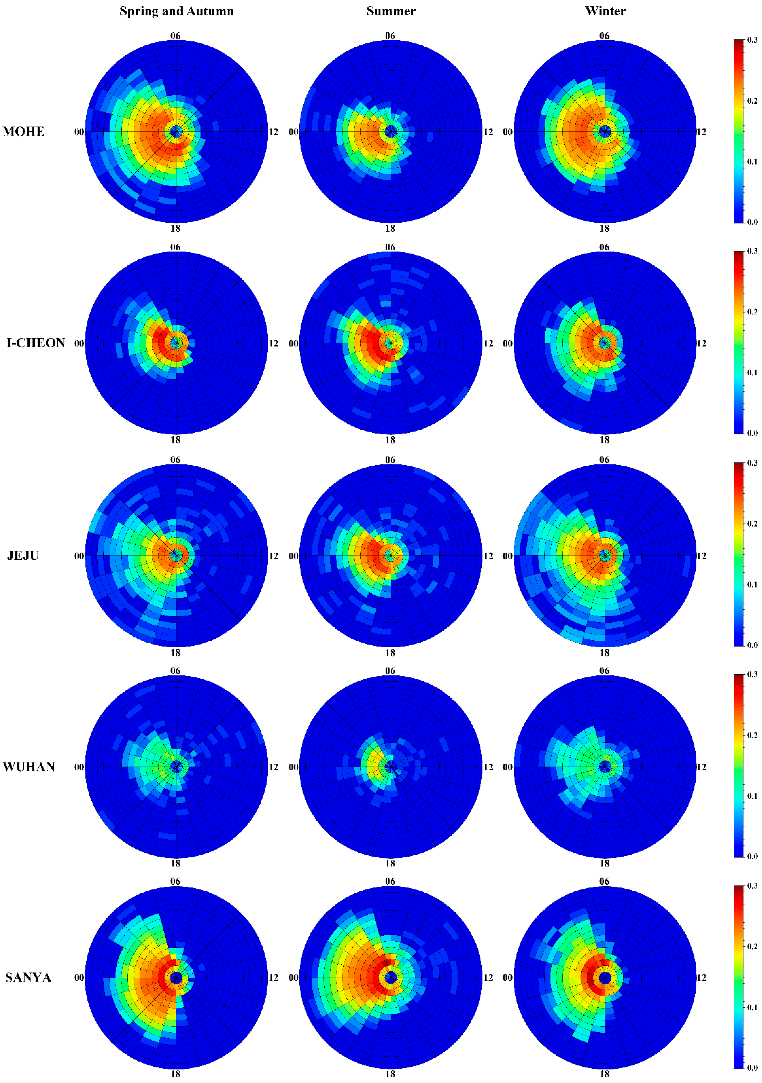
  • Our results showed that SF mainly occurs at the local nighttime and the occurrence rate of SF at Wuhan is evidently smaller than that at the other four stations. In addition, the occurrence rate of SF also shows an asymmetry in the nighttime: SF occurred more easily in the post-midnight hours when compared with the pre-midnight period, consistent with previous studies.
  • There is a peak of occurrence of SF in the summer in I-Cheon, Jeju, Sanya, and Wuhan; however, the Mohe station has the highest occurrence rate of SF in December. The different seasonal variations of SF might be due to the different geographic local conditions and formation mechanisms at these latitudes: Mohe is located inland at a mid-high latitude, so AGW which comes from the lower atmosphere should be different from that of other stations, contributing to the different seasonal characteristics of SF in these stations.
  • The most intense FSF appeared in the height range of 220–300 km in these stations, although there are different magnitude extensions in different region. Most FSF occurs during the post-midnight hours in the summer and is distributed more symmetrical around midnight in the winter in Mohe, I-Cheon, and Jeju. By contrast, it is more symmetrical around midnight in the summer at Sanya. As Sanya is located in the equatorial low latitudes, local ionospheric disturbances induced by atmospheric gravity waves and medium-scale traveling ionospheric disturbances (MSTIDs) induced by Perkins instability during the nighttime might contribute to the local time difference of SF in the summer.
  • The RSF mainly appeared in the frequency range of 1–7 Mhz with different magnitude extensions in different regions. In particular, the RSF covers a large frequency range of 1–13 Mhz in Sanya, and this phenomenon is most apparent in the equinox, indicating the frequently SSF occurrence in the equinox at Sanya. Moreover, the occurrence rate of mid-latitude SF reached its maximum in the midnight to post-midnight periods, confirming the previous results.
  • SF also appeared in the daytime in these stations, and AGW, TID, geomagnetic inclination/declination, etc. might contribute to the daytime SF formation. Due to the limitation of data, multi-instrument observations and simulations are needed to provide a statistical picture and to study the physical mechanisms of daytime SF in the future.

Author Contributions

Conceptualization, Y.Z. and J.F.; methodology, Z.Z.; investigation, C.Z. and Z.W.; validation, X.W. and B.C.; formal analysis, S.G. and Y.L.; resources, J.F. and S.G.; visualization, J.F. and Y, Z; funding acquisition, C.Z and X.W. All authors have read and agreed to the published version of the manuscript.

Funding

This work was supported by the National Key Research and Development Program of China (NO.2021YFC2802502), the Stable-Support Scientific Project of China Research Institute of Radio Wave Propagation (Grant No. A132102W06), the Hubei Natural Science Foundation (Grant No. 2022CFB651), the National Natural Science Foundation of China (NSFC Grant No. 42204161, 42074187), the Foundation of National Key Laboratory of Electromagnetic Environment (Grant No. 20200101), and the Excellent Youth Foundation of Hubei Provincial Natural Science Foundation (Grant No. 2019CFA054).

Data Availability Statement

Data sharing is not applicable to this article.

Acknowledgments

The authors would like to gratefully thank the anonymous reviewers for their insight and help. We appreciate the support by “The Young Top-notch Talent Cultivation Program of Hubei Province”.

Conflicts of Interest

The authors declare no conflict of interest.

References

  1. Booker, H.G. Turbulence in the ionosphere with applications to meteor trails, radio-star scintillation, auroral radar echoes, and other phenomena. J. Geophys. Res. 1956, 61, 673–705. [Google Scholar] [CrossRef]
  2. Ratcliffe, J.A. An Introduction to the Ionosphere and Magnetosphere; Cambridge University Press: Cambridge, UK, 1972. [Google Scholar]
  3. Booker, H.G.; Wells, H.W. Scattering of radio waves in the F region of ionosphere. Terr. Magn. Atmos. Electr. 1938, 43, 249. [Google Scholar] [CrossRef]
  4. Farley, D.T.; Balsley, B.B.; Woodman, R.F.; McClure, J.P. Equatorial SF, implications of VHF radar observations. J. Geophys. Res. 1970, 75, 7199–7216. [Google Scholar] [CrossRef]
  5. Sobral, J.H.A.; Abdu, M.A.; Zamlutti, C.J.; Batista, I.S. Association between plasma bubble irregularities and airglow disturbances over Brazilian low latitudes. Geophys. Res. Letts. 1980, 1, 980–982. [Google Scholar] [CrossRef] [Green Version]
  6. Abdu, M.A.; Batista, I.S.; Sobral, J.H.A. A new aspects of magnetic declination control on equatorial spread F and F region dynamo. J. Geophys. Res. 1992, 97, 14897–14904. [Google Scholar] [CrossRef] [Green Version]
  7. Abdu, M.A. Major phenomena of the equatorial ionosphere–thermosphere system under disturbed conditions. J. Atmos. Sol. Terr. Phys. 1997, 13, 1505–1519. [Google Scholar] [CrossRef]
  8. Abdu, M.A. Outstanding problems in the equatorial ionosphere– thermosphere system relevant to spread F. J. Atmos. Sol. Terr. Phys. 2001, 63, 869–884. [Google Scholar] [CrossRef]
  9. Abdu, M.A.; Kherani, E.A.; Batista, I.S.; Sobral, J.H.A. Equatorial evening prereversal vertical drift and spread F suppression by disturbance penetration electric fields. Geophys. Res. Lett. 2009, 36, L19103. [Google Scholar] [CrossRef] [Green Version]
  10. Huang, C.-S.; Kelley, M.C. Nonlinear evolution of equatorial spread F:1 On the role of plasma instabilities and spatial resonance associated with gravity wave seeding. J. Geophys. Res. 1996, 98, 15631–15642. [Google Scholar] [CrossRef]
  11. Huang, C.-S.; Foster, J.C.; Kelley, M.C. Long-duration penetration of the interplanetary electric field to the low-latitude ionosphere during the main phase of magnetic storms. J. Geophys. Res. 2005, 110, A11309. [Google Scholar] [CrossRef]
  12. Fejer, B.G.; Scherliess, L.; de Paula, E.R. Effects of the vertical plasma drift velocity on the generation and evolution of equatorial spread F. J. Geophys. Res. 1999, 104, 19854–19869. [Google Scholar] [CrossRef] [Green Version]
  13. Huba, J.D.; Joyce, G.; Krall, J. Three-dimensional equatorial spread F modeling. Geophys. Res. Lett. 2008, 35, L10102. [Google Scholar] [CrossRef]
  14. Tsunoda, R.T. On equatorial spread F: Establishing a seeding hypothesis. J. Geophys. Res. 2010, 115, A12303. [Google Scholar] [CrossRef]
  15. Yokoyama, T.; Shinagawa, H.; Jin, H. Nonlinear growth, bifurcation, and pinching of equatorial plasma bubble simulated by three-dimensional high-resolution bubble model. J. Geophys. Res. Space Phys. 2014, 119, 10474–10482. [Google Scholar] [CrossRef] [Green Version]
  16. Hysell, D.L.; Milla, M.; Kuyeng, K. Radio Beacon and Radar Assessment and Forecasting of Equatorial F Region Ionospheric Stability. J. Geophys. Res. Space Phys. 2019, 124, 9511–9524. [Google Scholar] [CrossRef]
  17. Wu, K.; Xu, J.Y.; Zhu, Y.J.; Yuan, W. Occurrence characteristics of branching structures in equatorial plasma bubbles: A statistical study based on all-sky imagers in China. Earth Planet. Phys. 2021, 5, 407–415. [Google Scholar] [CrossRef]
  18. Mohandesi, A.; Knudsen, D.; Skone, S.; Langley, R.; Yau, A. Altitude Distribution of Large and Small-Scale Equatorial Ionospheric Irregularities Sampled from an Elliptical Low-Earth Orbit. J. Geophys. Res. Space Phys. 2022, 127, e2021JA030104. [Google Scholar] [CrossRef]
  19. Dungey, J.W. Convective diffusion in the equatorial F region. J. Atmos. Terr. Phys. 1956, 9, 304–310. [Google Scholar] [CrossRef]
  20. Fejer, B.G.; Kelley, M.C. Ionospheric irregularities. Rev. Geophys. 1980, 18, 401–454. [Google Scholar] [CrossRef]
  21. Sultan, P.J. Linear theory and modeling of the Rayleigh-Taylor instability leading to the occurrence of equatorial spread F. J. Geophys. Res. 1996, 101, 26875. [Google Scholar] [CrossRef]
  22. Huba, J. Generalized Rayleigh-Taylor Instability: Ion Inertia, Acceleration Forces, and E Region Drivers. J. Geophys. Res. Space Phys. 2022, 127, e2022JA030474. [Google Scholar] [CrossRef]
  23. Woodman, R.F.; Hoz, C.L. Radar observations of F region equatorial irregularities. J. Geophys. Res. 1976, 81, 5447–5466. [Google Scholar] [CrossRef]
  24. Singh, S.; Johnson, F.S.; Power, R.A. Gravity wave seeding of equatorial plasma bubbles. J. Geophys. Res. 1997, 102, 7399–7410. [Google Scholar] [CrossRef] [Green Version]
  25. Tsunoda, R.T. Satellite traces: An ionogram signature for large-scale wave structure and a precursor for equatorial spread F. Geophys. Res. Lett. 2008, 35, L20110. [Google Scholar] [CrossRef]
  26. Aveiro, H.C.; Hysell, D.L.; Park, J.; Lühr, H. Equatorial spread F related currents: Three-dimensional simulations and observations. Geophys. Res. Lett. 2011, 38, L21103. [Google Scholar] [CrossRef] [Green Version]
  27. Perkins, F. Spread F and ionospheric currents. J. Geophys. Res. 1973, 78, 218–226. [Google Scholar] [CrossRef]
  28. Bowman, G.G. A review of some recent work on mid-latitude spread-F occurrence as detected by ionosondes. J. Geomagn. Geoelectr. 1990, 42, 109–138. [Google Scholar] [CrossRef] [Green Version]
  29. Yokoyama, T.; Yamamoto, M.; Fukao, S.; Cosgrove, R.B. Three dimensional simulation on generation of polarization electric field in the midlatitude E-region ionosphere. J. Geophys. Res. 2004, 109, A01309. [Google Scholar] [CrossRef]
  30. Balan, N.; Otsuka, Y.; Nishioka, M.; Liu, J.Y.; Bailey, G.J. Physical mechanisms of the ionospheric storms at equatorial and higher latitudes during the recovery phase of geomagnetic storms. J. Geophys. Res. 2013, 118, 2660–2669. [Google Scholar] [CrossRef]
  31. Zhou, C.; Tang, Q.; Huang, F.Q.; Liu, Y.; Gu, X.D.; Lei, J.H.; Ni, B.B.; Zhao, Z.Y. The simultaneous observations of nighttime ionospheric E region irregularities and F region medium-scale traveling ionospheric disturbances in midlatitude China. J. Geophys. Res. 2018, 123, 5195–5209. [Google Scholar] [CrossRef]
  32. Liu, Y.; Zhou, C.; Xu, T.; Wang, Z.K.; Tang, Q.; Deng, Z.X.; Chen, G.Y. Investigation of midlatitude nighttime ionospheric E-F coupling and interhemispheric coupling by using COSMIC GPS radio occultation measurements. J. Geophys. Res. 2020, 125, e2019JA027625. [Google Scholar] [CrossRef]
  33. Dabas, R.S.; Das, R.M.; Sharma, K.; Garg, S.C.; Devasia, C.V.; Subbarao, K.S.V.; Niranjan, K.; Rama Rao, P.V.S. Equatorial and low latitude spread-F irregularity characteristics over the Indian region and their prediction possibilities. J. Atmos. Sol. Terr. Phys. 2007, 69, 685–696. [Google Scholar] [CrossRef]
  34. Hoang, T.L.; Abdu, M.A.; MacDougall, J.; Batista, I.S. Longitudinal differences in the equatorial spread F characteristics between Vietnam and Brazil. Adv. Space Res. 2010, 45, 351–360. [Google Scholar] [CrossRef]
  35. Tulasi Ram, S.; Rama Rao, P.V.S.; Prasad, D.S.V.V.D.; Niranjan, K.; Gopi Krishna, S.; Sridharan, R.; Ravindran, S. Local time dependent response of postsunset ESF during geomagnetic storms. J. Geophys. Res. 2008, 113, A07310. [Google Scholar] [CrossRef] [Green Version]
  36. Balan, N.; Liu, L.; Le, H. A brief review of equatorial ionization anomaly and ionospheric irregularities. Earth Planet. Phys. 2018, 2, 1–19. [Google Scholar] [CrossRef]
  37. King, G.A. Spread-F on ionograms. J. Atmos. Terr. Phys. 1970, 32, 209–221. [Google Scholar] [CrossRef]
  38. Su, S.Y.; Yeh, H.C.; Heelis, R.A. ROCSAT 1 ionospheric plasma and electrodynamics instrument observations of equatorial spread F: An early transitional scale result. J. Geophys. Res. 2001, 106, 29513–29519. [Google Scholar] [CrossRef]
  39. Jin, H.; Zou, S.; Chen, G.; Yan, C.; Zhang, S.; Yang, G. Formation and Evolution of Low-Latitude F Region Field-Aligned Irregularities During the 7-8 September 2017 Storm: Hainan Coherent Scatter Phased Array Radar and Digisonde Observations. Space Weather 2018, 16, 648–659. [Google Scholar] [CrossRef]
  40. Reinisch, B.W.; Huang, X. Automatic calculation of electron density profiles from digital ionograms: 3. Processing of bottomside ionograms. Radio Sci. 1983, 18, 477–492. [Google Scholar] [CrossRef]
  41. Pezzopane, M.; Scotto, C. Automatic scaling of critical frequency foF2 and MUF(3000)F2: A comparison between Autoscala and ARTIST 4.5 on Rome data. Radio Sci. 2007, 42, RS4003. [Google Scholar] [CrossRef]
  42. Jiang, C.; Yang, G.; Zhao, Z.; Zhang, Y.; Zhu, P.; Sun, H. An automatic scaling technique for obtaining F2parameters and F1critical frequency from vertical incidence ionograms. Radio Sci. 2013, 48, 739–751. [Google Scholar] [CrossRef]
  43. Jiang, C.; Yang, G.; Zhou, Y.; Zhu, P.; Lan, T.; Zhao, Z.; Zhang, Y. Software for scaling and analysis of vertical incidence ionograms-ionoScaler. Adv. Space Res. 2017, 59, 968–979. [Google Scholar] [CrossRef]
  44. Pillat, V.G.; Guimaraes, L.N.F.; Fagundes, P.R. A computational tool for ionosonde CADI’s ionogram analysis. Comput. Geosci. 2013, 52, 372–378. [Google Scholar] [CrossRef]
  45. Pezzopane, M.; Pillat, V.; Fagundes, P. Automatic scaling of critical frequency foF2 from ionograms recorded at São José dos Campos, Brazil: A comparison between Autoscala and UDIDA tools. Acta Geophys. 2017, 65, 173–187. [Google Scholar] [CrossRef]
  46. Pillat, V.G.; Fagundes, P.R.; Guimarães, L.N.F. Automatically identification of Equatorial Spread-F occurrence on ionograms. J. Atmos. Sol. Terr. Phys. 2015, 135, 118–125. [Google Scholar] [CrossRef]
  47. Lan, T.; Zhang, Y.; Jiang, C.; Yang, G.; Zhao, Z. Automatic identification of Spread F using decision trees. J. Atmos Sol.-Terr. Phys. 2018, 179, 389–395. [Google Scholar] [CrossRef]
  48. Lan, T.; Hu, H.; Jiang, C.; Yang, G.; Zhao, Z. A Comparative Study of Decision Tree, Random Forest, and Convolutional Neural Network for Spread-F Identification. Adv. Space Res. 2020, 65, 2052–2061. [Google Scholar] [CrossRef]
  49. Scotto, C.; Ippolito, A.; Sabbagh, D. A method for automatic detection of equatorial spread-F in Ionograms. Adv. Space Res. 2019, 63, 337–342. [Google Scholar] [CrossRef]
  50. Rao, T.V.; Sridhar, M.; Ratnam, D.V. Auto-detection of sporadic E and spread F events from the digital ionograms. Adv. Space Res. 2022, 70, 1142–1152. [Google Scholar] [CrossRef]
  51. Hajkowicz, L. Morphology of quantified ionospheric range spread-F over a wide range of midlatitudes in the Australian longitudinal sector. Ann. Geophys. 2007, 25, 1125–1130. [Google Scholar] [CrossRef] [Green Version]
  52. Pezzopane, M.; Zuccheretti, E.; Abadi, P.; de Abreu, A.J.; de Jesus, R.; Fagundes, P.R.; Supnithi, P.; Rungraengwajiake, S.; Nagatsuma, T.; Tsugawa, T.; et al. Low-latitude equinoctial spread-F occurrence at different longitude sectors under low solar activity. Ann. Geophys. 2013, 31, 153–162. [Google Scholar] [CrossRef] [Green Version]
  53. Wang, G.; Shi, J.; Wang, X.; Shang, S.P. Seasonal variation of spread-F observed in Hainan. Adv. Space Res. 2008, 41, 639–644. [Google Scholar] [CrossRef]
  54. Lan, T.; Jiang, C.; Yang, G.; Zhang, Y.; Liu, J.; Zhao, Z. Statistical analysis of low-latitude spread F observed over Puer, China, during 2015–2016. Earth Planets Space 2019, 71, 138. [Google Scholar] [CrossRef]
  55. Guo, B.; Xiao, S.; Shi, J.; Xiao, Z.; Wang, G.; Cheng, Z.; Shang, S.; Wang, Z.; Suo, Y. Comparative study on characteristics of spread-F at low-and mid-latitudes during high and low solar activities over East Asia. Chin. J. Geophys. 2017, 60, 3289–3300. [Google Scholar] [CrossRef]
  56. Wang, N.; Guo, L.; Ding, Z.; Zhao, Z.; Xu, Z.; Xu, T.; Hu, Y. Longitudinal differences in the statistical characteristics of ionospheric spread-F occurrences at mid-latitude in Eastern Asia. Earth Planets Space 2019, 71, 47. [Google Scholar] [CrossRef]
  57. Lan, T.; Jiang, C.; Yang, G.; Sun, F.; Xu, Z.; Liu, Z. Latitudinal Differences in Spread F Characteristics at Asian Longitude Sector during the Descending Phase of the 24th Solar Cycle. Universe 2022, 8, 485. [Google Scholar] [CrossRef]
  58. Sun, W.; Xu, L.; Huang, X. Forecasting of ionospheric vertical total electron content (TEC) using LSTM networks. In Proceedings of the 2017 International Conference on Machine Learning and Cybernetics (ICMLC), Ningbo, China, 9–12 July 2017; pp. 340–344. [Google Scholar]
  59. Chen, Z.; Jin, M.; Deng, Y. Improvement of a Deep Learning Algorithm for Total Electron Content Maps: Image Completion. J. Geophys. Res. Space Phys. 2019, 124, 790–800. [Google Scholar] [CrossRef] [Green Version]
  60. Chen, X.; Lei, J.; Ren, D. A Deep Learning Model for the Thermospheric Nitric Oxide Emission. Space Weather 2021, 19, e2020SW002619. [Google Scholar] [CrossRef]
  61. Li, X.; Zhou, C.; Tang, Q. Forecasting Ionospheric foF2 Based on Deep Learning Method. Remote Sens. 2021, 13, 3849. [Google Scholar] [CrossRef]
  62. Xia, G.; Liu, M.; Zhang, F.; Zhou, C. CAiTST: Conv-Attentional Image Time Sequence Transformer for Ionospheric TEC Maps Forecast. Remote Sens. 2022, 14, 4223. [Google Scholar] [CrossRef]
  63. Jiang, C.; Zhang, Y.; Yang, G.; Zhu, P.; Sun, H.; Cui, X.; Song, H.; Zhao, Z. Automatic scaling of the sporadic E layer and removal of its multiple reflection and backscatter echoes for vertical incidence ionograms. J. Atmos. Sol. Terr. Phys. 2015, 129, 41–48. [Google Scholar] [CrossRef]
  64. Kohavi, R. Scaling Up the Accuracy of Naïve-Bayes Classifiers: A Decision-Tree Hybrid. In Proceedings of the Second International Conference on Knowledge Discovery and Data Mining, Portland, OR, USA, 2–4 August 1996; AAAI Press: Palo Alto, CA, USA, 1996; pp. 202–207. [Google Scholar]
  65. Piggot, W.R.; Rawer, K. URSI Handbook of Ionogram Interpretation and Reduction. In International Union of Radio Science; United States, Environmental Data Service: Washington, DC, USA, 1978. [Google Scholar]
  66. Chen, W.S.; Lee, C.C.; Chu, F.D.; Su, S.Y. Spread F, GPS phase fluctuations, and medium-scale traveling ionospheric disturbances over Wuhan during solar maximum. J. Atmos Sol. Terr. Phys. 2011, 73, 528–533. [Google Scholar] [CrossRef]
  67. Paul, K.S.; Haralambous, H.; Oikonomou, C.; Paul, A.; Belehaki, A.; Ioanna, T.; Kouba, D.; Buresova, D. Multi-station investigation of spread F over Europe during low to high solar activity. J. Space Weather Space Clim. 2018, 8, A27. [Google Scholar] [CrossRef] [Green Version]
  68. Bhaneja, P.; Earle, G.D.; Bullett, T.W. Statistical analysis of midlatitude spread F using multi-station digisonde observations. J. Atmos Sol.-Terr. Phys. 2018, 167, 146–155. [Google Scholar] [CrossRef]
  69. Igarashi, K.; Kato, H. Solar cycle variations and latitudinal dependence on the mid-latitude spread-F occurrence around Japan. In The XXIV General Assembly; International Union of Radio Science: Kyoto, Japan, 1993. [Google Scholar]
  70. Huang, W.Q.; Xiao, Z.; Xiao, S.G.; Zhang, D.H.; Hao, Y.Q.; Suo, Y.C. Case study of apparent longitudinal differences of spread F occurrence for two midlatitude stations. Radio Sci. 2011, 46, RS1015. [Google Scholar] [CrossRef]
  71. Devasia, C.V.; Jyoti, N.; Subbarao, K.S.V. On the plausible linkage of thermospheric meridional winds with equatorial spread F. J. Atmos. Sol. Terr. Phys. 2002, 64, 1–12. [Google Scholar] [CrossRef]
  72. Liu, Y.; Deng, Z.; Xu, T.; Kong, J.; Zhou, C.; Yao, Y. Daytime F region echoes at equatorial ionization anomaly crest during geomagnetic quiet period: Observations from multi-instruments. Space Weather 2022, 20, e2021SW003002. [Google Scholar] [CrossRef]
  73. Candido, C.M.N.; Batista, I.S.; Becker-Guedes, F.; Abdu, M.A.; Sobral, J.H.; Takahashi, H. Spread F occurrence over a southern anomaly crest location in Brazil during June solstice of solar minimum activity. J. Geophys. Res. 2011, 116, A06316. [Google Scholar] [CrossRef] [Green Version]
  74. Shi, J.K.; Wang, G.J.; Reinisch, B.W.; Shang, S.P.; Wang, X.; Zherebotsov, G.; Potekhin, A. Relationship between strong range spread F and ionospheric scintillations observed in Hainan from 2003 to 2007. J. Geophys. Res. 2011, 116, A08306. [Google Scholar] [CrossRef]
  75. Li, J.; Ma, G.; Maruyama, T.; Li, Z. Mid-latitude ionospheric irregularities persisting into late morning during the magnetic storm on 19 March 2001. J. Geophys. Res. 2012, 117, A08304. [Google Scholar] [CrossRef]
  76. Kil, H.; Lee, W.K.; Paxton, L.J. Origin and distribution of daytime electron density irregularities in the low-latitude F region. J. Geophys. Res. Space Phys. 2020, 125, e2020JA028343. [Google Scholar] [CrossRef] [PubMed]
  77. Jiang, C.; Yang, G.; Liu, J.; Yokoyama, T.; Komolmis, T.; Song, H. Ionosonde observations of daytime spread F at low latitudes. J. Geophys. Res. Space Phys. 2016, 121, 12093–12103. [Google Scholar] [CrossRef]
  78. Yang, G.; Jiang, C.; Lan, T.; Huang, W.; Zhao, Z. Ionosonde observations of daytime spread F at middle latitudes during a geomagnetic storm. J. Atmos. Terr. Phys. 2018, 179, 174–180. [Google Scholar] [CrossRef]
  79. Xiao, S.; Shi, J.; Zhang, D.; Hao, Y.; Huang, W. Observational study of daytime ionospheric irregularities associated with typhoon. Sci. China Technol. Sci. 2012, 55, 1302–1304. [Google Scholar] [CrossRef]
  80. Huang, C.S.; de La Beaujardier, O.; Roddy, P.A.; Hunton, D.E.; Ballenthin, J.O.; Hairston, M.R. Long-lasting daytime equatorial plasma bubbles observed by the C/NOFS satellite. J. Geophys. Res. 2013, 118, 2398–2408. [Google Scholar] [CrossRef]
Figure 1. Geographical locations of the selected ionosondes.
Remotesensing 15 01108 g001
Figure 2. (a) An example of consecutive points (feature value) extraction positions in ionogram without SF in Mohe at 03:15UT on 9 January 2017. (b) An example of consecutive points (feature value) extraction position in ionogram with SF in Wuhan at 17:45UT on 26 June 2015.
Remotesensing 15 01108 g002aRemotesensing 15 01108 g002b
Figure 3. The interface of training naive Bayesian classifier using Weka Explorer.
Remotesensing 15 01108 g003
Figure 4. Occurrence rate of SF at Mohe, I-Cheon, Jeju, Wuhan, and Sanya according to the 0–24 LT and January–December division.
Remotesensing 15 01108 g004
Figure 5. Frequency spread-F (FSF) index distribution in summer, winter, and equinox (spring and autumn) in Mohe, I-Cheon, Jeju, Wuhan, and Sanya, which is binned into the function of local time 0:00–24:00 LT and heights 200–500 km within a grid of 1 h × 20 km.
Remotesensing 15 01108 g005
Figure 6. Seasonal distribution of RSF index in Mohe, I-Cheon, Jeju, Wuhan, and Sanya within the same grid as Figure 5.
Remotesensing 15 01108 g006
Table 1. The geographical coordinates of the selected stations.
StationGeographic Latitude/°Geographic Longitude/°Geomagnetic Latitude/°
Mohe52.00122.5242.68
I-Cheon37.14127.5428.07
Jeju33.43126.3024.31
Wuhan30.50114.4020.99
Sanya18.34109.428.82
Table 2. Data availability of the selected ionosonde stations during the period of 2009–2018.
StationData Period Data Missing Period
Mohe2013–2018January~August in 2013, May~December in year 2018
I-Cheon2010–2013November and December in 2013
Jeju2009–2013July, November, and December in 2013
Wuhan2013–2018/
Sanya2013–2017August in 2013, December in 2016, January, March, May, and June in 2017
Disclaimer/Publisher’s Note: The statements, opinions and data contained in all publications are solely those of the individual author(s) and contributor(s) and not of MDPI and/or the editor(s). MDPI and/or the editor(s) disclaim responsibility for any injury to people or property resulting from any ideas, methods, instructions or products referred to in the content.

