Technical Note

Polarization Orientation Method Based on Remote Sensing Image in Cloudy Weather

1
College of Optoelectronic Engineering, Chongqing University of Posts and Telecommunications, Chongqing 400065, China
2
Chongqing Academy of Metrology and Quality Inspection, Chongqing 401121, China
*
Author to whom correspondence should be addressed.
Remote Sens. 2023, 15(5), 1225; https://doi.org/10.3390/rs15051225
Submission received: 10 January 2023 / Revised: 9 February 2023 / Accepted: 21 February 2023 / Published: 22 February 2023

Abstract

:
Autonomous navigation technology is a core technology for intelligent operation, allowing the vehicles to perform tasks without relying on external information, which effectively improves the concealability and reliability. In this paper, based on the previous research on the bionic compound eye, a multi-channel camera array with different polarization degrees was used to construct the atmospheric polarization state measurement platform. A polarization trough threshold segmentation algorithm was applied to study the distribution characteristics and characterization methods of polarization states in atmospheric remote sensing images. In the extracted polarization feature map, the tilting suggestion box was obtained based on the multi-direction window extraction network (similarity-based region proposal networks, SRPN) and the rotation of the suggestion box (Rotation Region of interests, RRoIs). Fast Region Convolutional Neural Networks (RCNN) was used to screen the suggestion boxes, and the Non-maximum suppression (NMS) method was used to select the angle, corresponding to the label of the suggestion box with the highest score, as the solar meridian azimuth in the vehicle coordinate system. The azimuth angle of the solar meridian in the atmospheric coordinate system can be calculated by the astronomical formula. Finally, the final heading angle can be obtained according to the conversion relationship between the coordinate systems. By fitting the measured data based on the least Square method, the slope K value is −1.062, RMSE (Root Mean Square Error) is 6.984, and the determination coefficient R-Square is 0.9968. Experimental results prove the effectiveness of the proposed algorithm, and this study can construct an autonomous navigation algorithm with high concealment and precision, providing a new research idea for the research of autonomous navigation technology.

Graphical Abstract

1. Introduction

Living things are the most outstanding works of art in nature, and they are also the inexhaustible source of human academic ideas, engineering principles, and inventions. It has been found that some insects and crustaceans in nature have small and fully functional compound eyes. They have the advantages of small size, high sensitivity, and a large field of view, and they can sense the sky polarization vector field information by using the polarization structure of compound eyes to obtain excellent navigation and positioning ability. The 21st century is an age of information, and the demand for accurate autonomous navigation and positioning technology is increasingly urgent. Especially for military facilities, there are strict requirements for accuracy, concealment, and anti-interference. Different from traditional radio navigation technology [1], autonomous navigation technology can achieve accurate positioning and navigation of the carrier without relying on external information interaction, but only on its own sensing equipment, thus effectively improving the concealability and anti-interference ability of the vehicle and playing an important role in the military field.
The proposed bionic polarization navigation technology is based on many scholars’ in-depth research on the principle of insect navigation and positioning. It has been found that the beam structure formed by microvilli in a compound eye has photosensitive and angular resolution characteristics. The beam with two or more groups of mutually perpendicular microvillus has the ability to sense polarized light. These structures, called dorsal rim area (DRA), are distributed in the region of the back edge of the compound eye and are capable of collecting information about the atmospheric polarization state. The angle between the body axis and the solar meridian is calculated by combining the polarization-sensitive neurons to realize positioning and navigation [2]. By studying the collecting behavior of bees, researchers found that bees can distinguish the polarization direction (E vector) of the received sky polarized light relative to the position of the sun [3,4], which provides a method for positioning by using the atmospheric polarization state (Figure 1).
Wehner et al. conducted a test in a cloudy climate with an ultraviolet band, analyzed the relationship between the polarization distribution pattern and the position of the sun [5], and compared the atmospheric polarization distribution information in sunny and cloudy climates by using the whole-sky imaging polarization measurement. Although the degree of polarization in a cloudy sky is significantly different from that in a clear sky, the polarization angle does not change significantly. W.Z. et al. used a large-field camera to collect atmospheric polarization state information, studied the polarization angle distribution of atmospheric polarized light in different weather conditions, and proved, through experiments, that polarization navigation has better robustness and navigation accuracy in different weather conditions [6]. As the phenomenon of atmospheric aerosol high load is relatively serious in Asia, the research team of Hefei University of Technology [7] studied the change of atmospheric polarization state under the condition of high load aerosol in cities. The study found that high-load aerosols would change the original symmetrical distribution of atmospheric polarization state and make the actual symmetry line deflect and generate an angle between the solar meridians. J.C. et al. [8] studied the characteristics of atmospheric polarization distribution at sea, based on the Rayleigh scattering theory, and found that the atmospheric polarization distribution was influenced by both the sun and the moon, and the weight values of both changed over time. Based on the Rayleigh scattering model, Hamaoui [9] proposed a polarized light navigation method based on gradient operator and studied the impact of measurement errors and atmospheric condition changes on measurement results. However, the long-term stability study was lacking. Samuel et al. [10] conducted an in-depth study of underwater polarization modes, extended the study of polarization navigation mechanism to underwater, and opened up new possibilities for underwater long-distance navigation.
With the further study of the navigation mechanism, the real-time acquisition equipment of the atmospheric polarization state is also being developed. At present, the research on polarization sensing structure mainly falls into three categories. The first is a polarization direction analyzer composed of multiple pairs of linear polarizers and photodetectors. The second type is a polarization imaging camera with a large field of view. The third type is a polarization sensor array of the focal plane. At the end of last century, Swedish scientist Lambrinos et al. [11] studied the polarization navigation mechanism of sand ants and realized the solution of the heading angle by using four groups of polarization direction analyzers. Chahl J et al. [12] took a dragonfly compound eye as the prototype, integrated the single eye with the polarization sensor, and fixed it on the rolling axis of the bionic robot to more accurately control the rolling angle in the forward process. Julien et al. [13] proposed an astronomical compass based on UV skylight line polarization. As the main polarization navigation structure, the navigation principle of the compass is to use the single point polarization information to solve the heading angle. Due to the small field of view, the amount of information required for collection and analysis is small, and it is easy to be affected by obstacles and strong environmental light, which will reduce the accuracy of navigation or cause navigation failure. In addition, it is necessary to cooperate with other sensing equipment to obtain complete navigation information. Miyazaki et al. [14] fixed the fisheye lens and CCD camera on the rotating table, to observe and calculate the changes of atmospheric polarization state between 0 and 180°. Inspired by the sand ant, Du T. et al. [15,16] proposed a multi-sensor fusion positioning and map rendering method. The polarization skylight sensor design can effectively reduce positioning errors and detection time, but the multi-sensor design also makes the device too large. Sarkar et al. [17,18] developed a 128 × 128 pixel focal plane polarization sensor through the 180 nm process, which was composed of four kinds of linear gate polarizers with the polarization direction spaced 45° apart. WANG et al. [19] proposed a bionic polarization camera consisting of four cameras, which realized real-time image-based polarization measurement. The heading angle of the camera was calculated using the skylight polarization pattern, and the maximum orientation error, based on the angle of polarization (AOP), is just 0.5 degrees. Based on this structure, the real-time variation law of polarization information with the angle position of incident polarized light was studied. Compared with the first type of single-point polarization information measurement, the latter two types of structures have more accurate orientation information and anti-interference ability through the polarization information in the large field of view, but at the same time, the amount of data required to process is larger, and the polarization structure is more complex and huge.
In conclusion, the bionic polarized light navigation method is still in the research stage. It is a research hotspot in the field of autonomous navigation and positioning, and there are still many key problems to be solved. Inspired by the bionic compound eye structure, this paper constructs a polarization measurement platform to collect a large number of atmospheric polarization remote sensing images. Based on the low polarization threshold, similarity-based region proposal networks (SPRN), Rotation Region of Interests (RRoIs), and Fast Region Convolutional Neural Networks (RCNN), the heading angle of the vehicle is calculated. It provides a new research idea for autonomous navigation technology.

2. Polarization Navigation Algorithm

Rayleigh scattering model has a high similarity with the actual atmospheric polarization model and is the most classical characterization method to describe the atmospheric polarization under ideal conditions. The distribution of atmospheric polarization modes described by Rayleigh scattering is shown in Figure 2.
In the Figure 2, O is the ground observation point, Z is the zenith point, S is the sun, SM represents the solar meridian, ASM represents the inverse solar meridian, and the position and thickness of the short line represent the vibration direction and polarization degree of the scattered light E vector, respectively. The atmospheric polarization pattern has remarkable symmetry. The e-vector direction is antisymmetric with respect to the solar meridian plane determined by the observation point, the sun and the zenith, while the polarization degree is symmetric with respect to the solar meridian plane.
According to the Rayleigh scattering model, the distribution of atmospheric polarization is centered on the sun and changes with the motion of the sun. Although the position of the sun regularly moves with the change of time and observation site, the sky polarization pattern, corresponding to a certain position at a certain time, is stable.
Therefore, the sun position information obtained from the atmospheric polarization mode can provide a reference for navigation, and the position change of the solar meridian can be used to solve the two-dimensional plane heading angle.

2.1. Image Description of Polarization Mode

Stokes vector model is one of the most commonly used methods to describe polarization. The Stokes vector of incident light is expressed as shown below:
I φ = 1 2 I + Q c o s 2 φ + U s i n 2 φ
where  I φ  represents the incident light intensity when the polarization direction is  φ , I is the sky light intensity, Q is the polarized light component in the direction of 0°, and U is the polarized light component in the direction of 45°.
Therefore, as long as three or more  φ  angles are known, the I, Q, and U components in the original sky can be obtained according to the above equation. The three polarization directions of 0°, 45°, and 90° were selected to obtain the following equations:
I = I 0 + I 90 Q = I 0 I 90 U = 2 I 45 I 0 I 90
The intensity of light in different polarization directions can be obtained by using grayscale graphs. After the Stokes vector is solved, the degree of polarization image (DOP) and angle of polarization image (AOP) are calculated as follows:
D O P = Q 2 + U 2 I A O P = 1 2 a r c t a n U Q
DOP represents the sky polarization state, AOP is the angle between the polarization direction vector of the sky observation point in the carrier coordinate system and the body axis of the carrier (camera). According to the Rayleigh scattering principle, the atmospheric polarization mode is symmetrical about the solar meridian passing through the sun and zenith, and its polarization degree is symmetrical about the solar meridian distribution. Where the axis of symmetry is located, the degree of polarization is maximum, and the farther away from the axis of symmetry, the smaller the degree of polarization. In the DOP, there will be two polarization low points along the symmetry axis. In this paper, the algorithm is designed according to the feature that the center of the two polarization low points in the DOP is on the solar meridian.

2.2. Solar Azimuth Acquisition in the Carrier Coordinate System

In this paper, the center of gravity of the carrier is taken as the origin O, the direction opposite to the carrier course is taken as the X-axis, and the direction perpendicular to the carrier course is taken as the Y-axis, and the carrier coordinate system, as shown in Figure 3, is established.
The solar azimuth angle in the carrier coordinate system is the deflection angle of the solar meridian in the ontological coordinate system. In this paper, the calculation method of carrier azimuth  φ 0  is shown in Figure 4, which mainly includes feature extraction, multi-directional window extraction network (SRPN), and improved suggestion box rotation module (RRoIs).
Firstly, the threshold segmentation is used to extract the features of the DOP image, and the polarization trough is extracted. Feature points are defined as pixel points satisfying Equation (4):
D O P < θ t h = m i n D O P + τ
where  θ t h  and  τ  represent the feature threshold and threshold correction value, respectively. Figure 5 shows the feature map extracted based on the threshold of the trough of DOP.
As shown in Figure 5a, threshold segmentation was used to find the trough of polarization in remote sensing images. The value of the threshold  θ t h  was calculated dynamically to meet the need of extracting enough feature points. As shown in Figure 5e, the points in the figure whose DOP value was less than the threshold were extracted as trough of polarization.
In order to obtain the azimuth information, the region of interest of the feature map was processed based on SRPN [20] and RRoIs [21]. SRPN is an improvement on traditional region proposal network (RPN) [22] and is mainly used to improve the extraction effect of a vertical suggestion box. RPN is usually used to generate high-quality object recommendations, which are critical to improving the performance of the detector. In traditional RPN, anchor points are defined by their dimensions and aspect ratio. A group of anchor points, with different dimensions and aspect ratios, is needed to obtain enough positive samples with high Intersection over Union (IOU, the overlap rate between the target window predicted by the model and the original labeled window) ratios with the target object. However, because the sampling is too intensive, the imbalance between foreground and background will be aggravated, leading to the deterioration of module performance. In addition, for tiny objects, the IOU ratio is usually too small to reach the set threshold. Therefore, most small samples will be regarded as negative samples and ignored during training. To solve these problems, we designed the S-RPN network to provide high quality advice. Sparse sampling method was adopted, and only one anchor point was sampled at each position of the feature map, which was nine times less than the original RPN.
The main structure diagram of the model is shown in Figure 6.
Firstly, a sliding window was used to generate multiple anchor boxes with different aspect ratios on the feature map, and then, the candidate anchors corresponding to the original receptive field were obtained through the boxes of different sizes. In this paper, IOU calculation was used to classify candidate anchors:
I O U = A B A B
where A is the extracted suggestion box, and B is the real label window provided by the training set. Location correction for the Bounding Box, classified as prospects, is:
d P = W T · C P
where  d P  represents the objective function to be predicted,  W  is the training parameter, and C(P) is the feature vector of the candidate suggestion box.
Finally, coordinate correction and score sequencing of Anchor candidates were conducted. The candidate Anchor with high scores was selected as the suggestion box, and its four coordinates {x,y,w,h} were returned by regression operation.
As shown in Figure 7, the suggestion box generated by SRPN algorithm is a horizontal rectangular box, which cannot provide direction information. Therefore, based on the improvement of the RoI Pooling [23], this paper designed an algorithm (composed of Rotation RoIs and Fast RCNN modules) to rotate the above suggestion box and obtain a tilted suggestion box:
x , y , w , h x , y , w , h , φ 0
Firstly, the Rotation RoI (RRoI) was used to add the angle information to the horizontal rectangular box. Each horizontal anchor box generated by SRPN was passed as input to the RRoI layer. In this paper, RoI Align was used to replace traditional RoI pooling to reduce the dimension of the feature map, and a single fully connected layer was merged into 10 channels, significantly improving the computing speed. RoI Align uses bilinear interpolation to process the feature map where the proposal is located to avoid feature inaccuracies caused by boundaries. In addition, it preserves the fractional portion of the proposal mapped to the feature map location. Therefore, the effect of using RoI Align during target detection is better than that of RoI Pooling, especially for the accuracy of small targets. ROI Align returns the horizontal Anchor to a rotating result, as shown in Figure 7, where (x,y) is the central coordinate of the rotation suggestion frame, w and h are the width and height of the suggestion frame, respectively, and  φ 0  is the rotation angle.
These suggestion boxes were then crossed with the actual labels marked in the training set, and gravity fit was calculated.
Finally, the non-maximum suppression (NMS) method [24] was used to screen the suggestion boxes and select the angle of the label corresponding to the suggestion box with the highest score as the detection result. As a common functional module in Faster R-CNN [25], NMS is widely used in object detection, whose purpose is to eliminate redundant boxes and find the best location for object detection. Faster R-CNN is a classical deep learning algorithm, which has high recognition accuracy and recognition efficiency, and it has a good recognition rate for large target areas. NMS performs a local maximum search on all boxes obtained by the Faster R-CNN detection module to search for the maximum value in a neighborhood to filter out a part of boxes and improve the final detection accuracy, sort the scores of all boxes, and select the box with the highest score. The remaining boxes were traversed, and if the IOU with the current highest dividing box was greater than a certain threshold, the box was deleted. The process continues by picking the box with the highest score from the unprocessed box and repeating the process until the final result is obtained. The  φ 0  extracted by the final result is the azimuth angle of the solar meridian in the carrier coordinate system.

2.3. Solar Azimuth Acquisition in the Navigation Coordinate System

In order to visually display the influence of each parameter on the measurement in the navigation coordinate system, as shown in Figure 8, a rectangular coordinate system was established with the due north direction as the X axis, the due east direction as the Y axis, and the vertical line across the zenith as the Z axis. The navigation reference coordinate system was obtained by projecting the three-dimensional space coordinate system onto the two-dimensional plane.
The solar azimuth  φ s  starts from true north and is positive clockwise. Its value ranges from 0 to 360 degrees. In the celestial coordinate system, solar angle  α , solar declination angle  δ , true solar time  S t  and solar hour angle T are introduced, and the theoretical positions of zenith angle and solar azimuth angle are obtained by astronomical related formulas.
The calculation of solar altitude angle and azimuth angle is usually based on the coordinate system of equator, ecliptic, and horizon as shown in Figure 9, and the spherical trigonometric formula is used for formula derivation. Several high-precision (≤0.01°) complex algorithms mentioned in literature [26,27,28] are basically different approximations of the same astronomical algorithm. Solar declination and hour angle can be obtained from these approximately calculated parameters, and then, solar altitude angle and azimuth angle can be calculated. These are theoretical calculations without loss of accuracy. If the astronomical high precision measured values of these parameters can be obtained directly, the actual solar altitude angle and azimuth angle can be calculated directly.
The specific calculation process of the sun position was as follows.
Calculation of daily angle α:
α = 2 π D D o / 365.24
D o = 79.6764 + 0.2422 × y 1985 f l o o r y 1985 / 4
where D is the product day of the year, that is, the number of days from 1 January of the year, y is the current year, and floor is the downward integral function.
Calculation of solar declination angle  δ :
δ = 0.3723 + 23.2567 sin α + 0.1149 sin 2 α 0.1712 sin 3 α 0.758 cos α + 0.3656 cos 2 α + 0.0201 cos 3 α
To calculate true solar time  S t , first calculate local solar time  S d :
S d = S o + F o 120 ° J D + J F / 60 × 4 / 60  
where  S o  and  F o  are the hours and minutes of the local time zone of the observation point, respectively, and  J D  and  J F  are the longitude and arc min of the observation point, respectively.
Then, the time difference  E t  can be calculated from the daily angle α:
E t = 0.0028 1.9857 sin α + 9.9059 sin 2 α 7.0924 cos α 0.6882 cos 2 α
The true solar time  S t  is modified by the time difference  E t :
S t = S d + E t / 60
According to the calculation result of true solar time  S t , the hour angle of true sun T can be calculated:
T = S t 12 × 15 °
Finally, the solar altitude angle  θ s  and the solar azimuth angle  φ s  can be calculated according to the following formula:
sin ( π 2 θ s ) = sin δ sin L + cos δ cos L cos T
cos ( φ s + π ) = ( sin ( π 2 θ s ) sin L sin δ ) / cos ( π 2 θ s ) cos L
where, L is the local latitude.

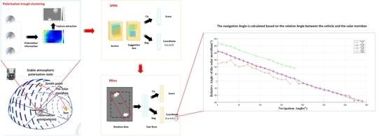
2.4. Course Angle Calculation

The carrier coordinate system and navigation coordinate system have been established in the previous section. The position of the solar meridian in the corresponding coordinate system was obtained. In this paper, using the solar meridian as the intermediate bridge, the position change of the solar meridian can be used to solve the two-dimensional plane heading angle.
In Figure 10, the navigation coordinate system takes the ground observation point as the origin O, the geographical due north direction as the Y axis, and the geographical due east direction as the X axis. The carrier coordinate system takes the carrier as the origin O, the direction opposite to the course is the X-axis, and the direction perpendicular to the course is the Y-axis. The origin of the navigation coordinate system overlapped with that of the carrier coordinate system. Based on the position of the sun meridian in the navigation coordinate system, the carrier coordinate system was drawn in the navigation coordinate system. Given that  φ 0  is the azimuth angle of the solar meridian in the carrier coordinate system and  φ s  is the azimuth angle of the solar meridian in the navigation coordinate system, the heading angle  φ c  in the navigation coordinate system can be obtained.
When the measured  φ 0  is greater than 180°, the range is converted to [0, 180] by subtraction  φ 0  from 360°. In this case, the value converted by  φ s  minus  φ 0  is the direction of the carrier coordinate system X axis. As shown in Figure 7, since the carrier’s driving direction is opposite to the X-axis direction, adding 180° to the result is the heading angle  φ c  in the navigation coordinate system. Correspondingly, when  φ 0  is less than 180°,  φ c  can be calculated by summing up  φ s ,   φ 0 , and 180°. In particular, when  φ 0    = 180°,   φ c    =  φ s .
φ c = φ s 360 ° φ 0 + 180 °   φ 0 > 180 ° φ s + φ 0 + 180 °   φ 0 < 180 ° φ s   φ 0 = 180 °
The mathematical model of carrier’s driving direction and solar meridian relative angle was established according to the deflection relation. In the clockwise direction, the relation between the angle of the carrier’s driving direction and the angle of the solar meridian is as follows:
Δ θ = k Δ φ c + Δ φ s + σ
where  Δ θ  is the angle of the solar meridian,  Δ φ c  is the angle of the camera,  Δ φ s  is the deflection of the solar meridian itself over time, and σ is the random disturbance.

3. Experiment and Discussion

3.1. Measurement Platform Based on Bionic Compound Eye

Previous research on the compound eyes of insects in nature have shown that the beam of compound eyes has photosensitivity and angular resolution characteristics. In addition, the beam with two or more groups of perpendicular microvillus structures is capable of sensing polarized light, giving it the ability to navigate. Inspired by the principle of compound eye imaging, a polarization measuring platform was constructed in this paper. The measuring platform mainly consists of a camera array, electric rotating head, fixed bracket, polarizer fixer, and linear polarizer.
According to the image description of the polarization mode, it is necessary to add a polarizer in front of the camera lens in order to capture the polarizing image. In this paper, a polarization acquisition device is composed of a fixed part of a polarizer, a camera array, and a linear polarizer with different polarization directions, as shown in Figure 11.

3.2. Measurement Test and Data Analysis

The experimental data were collected from March to September 2022 in mostly cloudy weather at Chongqing University of Posts and Telecommunications (482.7 m above sea level) with coordinates of 29°31′55.62″ north latitude and 106°36′18.4″ east longitude. At the beginning of the experiment, the X-axis of the carrier coordinate system pointed due south. Then, it rotated clockwise, and the sky polarization map of 0°, 45°, and 90° were collected simultaneously. A total of 3600 images were collected from March to September of this year under sunny, cloudy, and rainy weather. The image resolution is 1920 × 1080 (part of them is 3000 × 4000), and both vertical and horizontal resolutions are 96 dpi (part of them is 72 dpi). The data set in this paper consists of the sky polarization images, with a total of 3600 images, 3000 of which are the training set and 600 of which are the test set (Table 1). In the production of the dataset, the images of different weather, different seasons, and times are specially collected to ensure the applicability and diversity of the dataset. For the collected data set, we use the same format as VOC2007 for annotation, and the specific steps are as follows. First, we use the batch tool to format and name all the images we have captured. Then, the lableImg tool is used to annotate the image by drawing the targets in the image with boxes and saving the format as XML. Finally, we put the labeled training and test images into their own folders and write the names, in order, into a TXT document. When this is done, a complete dataset of buildings is made. We can train the obtained remote sensing polarization image dataset, and then obtain the recognition model of the polarization map.
Figure 12 shows the atmospheric polarization image collected in the experiment and the corresponding processing results. Due to space constraints, only partial results are shown in Figure 12. In the following data analysis, the relevant data will be fully listed.
Columns 1–3 in Figure 12 are original images of polarization directions 0°, 45°, and 90°. The fourth column is the angle of polarization (AOP) image after pseudo-color processing. The fifth column is the degree of polarization (DOP) image after pseudo-color processing. The sixth column is the feature point clustering map after feature extraction of DOP. In addition, those figures also show the results of the rotation suggestion box. It is not difficult to see, from the AOP and DOP in the figure, that they both change regularly as the vehicle traveling angle changes. The feature extraction and angle characterization of DOP are more significant and effective. This is also the basis for choosing DOP as angle calculation in this paper.
Table 2 shows the actual rotation angle of the carrier measured since 13:26 on 7 September 2022 and the results obtained by the algorithm in this paper. The data were analyzed, and the results were drawn, as shown, in the figure below. From left to right are the original data graph, the data graph after the removal of abnormal points, and the difference graph of the latter term.
As can be seen from Figure 13, in cloudy weather, the calculated relative angle of the solar meridian presents a piecewise linear relationship, in which the variation range of the transmutation point is about 180°. According to the previous research and analysis, the abrupt change of angle is caused by the ambiguity of the solar meridian [29]. Due to the abrupt change of 180° in the calculated solar meridian data, translation processing was carried out in this paper to make the data distribute continuously. According to the RANSAC random consistency sampling principle, the least square method was used to fit the model and evaluate it. The fitting effect was shown in Figure 14, and the fitting effect evaluation index and fitting k value were shown in Table 3.
The R2 of the data fit was above 0.99, indicating that the fitting effect was very good and the model was consistent with the actual results.
To further verify the correctness of the model, researchers conducted experiments in different time periods and weather conditions. According to the results in Figure 15, in general, the navigation angle has a linear relationship with the solar meridian angle. As time changes, the calculation results in a time offset such that the fitted curve is translated up and down in the coordinate system. When the weather changes, the calculated results are generally close to each other in sunny and cloudy days. However, in some extreme cases, especially when fog covers part of the atmospheric polarization distribution, the measurement results will have large deviations.
In general, the predicted results of the model are consistent with the actual rotation of the camera angle, so it is feasible to use the model for navigation and orientation in cloudy weather.

3.3. Disscussion

In this paper, it has been found that the polarization information in atmospheric remote sensing images is helpful for the autonomous navigation of vehicles. Based on SRPN and RRoIs, the solar meridian azimuthal angle can be calculated from the AOP feature map. Combined with the transformation relationship between coordinate systems, the final heading angle can be obtained.
Compared with the mainstream GPS navigation, geomagnetic navigation, inertial navigation and other technologies, the advantage of this method is that the vehicles can quickly obtain the heading angle only from the atmospheric remote sensing image without interacting with the outside world. This method has high concealment and is not affected by cumulative errors. It can be divided into three categories according to the measuring device and data processing method.
The first kind of method [11] is the mainstream polarization navigation structure at present. Its navigation principle is to use single point polarization information to solve heading angle. The specific structure of the measurement is four groups of analysers with polarization direction difference of 45°. A single array of analyzers consists of a pair of polarizers perpendicular to each other, a photodetector, and a logarithmic amplifier. After A/D conversion, signal processing and calculation, the course angle information is transmitted to the upper computer through the serial port. This kind of method requires less information to be collected and analyzed, but its field of view is small and easy to be affected by obstacles and environmental strong light, which will reduce navigation accuracy or cause navigation failure. In addition, it needs to cooperate with other sensing equipment to obtain complete navigation information.
In order to solve the problem that the acquisition device of the first kind of method is too large, the polarization sensor of focal plane is developed by micro-nano process [17,18]. The sensor is composed of four linear grid polarizers with polarization directions 45° apart. Based on this structure, the real-time variation of polarization information with the Angle of incident polarized light is studied. The structure of the sensor is closer to the biological compound eye, but at the same time, the measurement structure is precise and complicated, and it is difficult to solve the measurement error caused by environmental change.
The method adopted in this paper belongs to the third category, that is, the wide-angle lens is used to capture the atmospheric polarization information under the large field of view, and the neural network algorithm is used to realize the polarization information solution. The theoretical basis of this method comes from the distribution of atmospheric polarization states, so the real-time calculation results are easy to be affected by the abrupt change of climate. In addition, in some extreme weather, the accuracy will be greatly affected. However, the training model based on big data can effectively improve the robustness of the algorithm and cope with certain sudden environmental factors. In addition, since there is no cumulative error in this method, even if the measurement error occurs at one time, it can be immediately corrected in the subsequent measurement. In previous studies, Tang J et al. used PCNN (Pulse Coupled Neural Network) to denoise the collected polarization map, and extracted the solar meridian from the AOP image to calculate the navigation angle [30]. Its study was carried out under different experimental conditions, and the average error was no more than 1.41° in several cases. In order to estimate the heading angle of the camera by using the skylight polarization pattern, Wang Y et al. establish the sun vector as an optimization problem to find the minimum eigenvector [19]. The solar meridian is estimated from the DOP pattern by detecting the reflection symmetry axis. Its average orientation error based on AOP is about 0.012°. The measurement methods of the above two static environments have high measurement accuracy, but there is still a lack of continuity and immediacy in the measurement. The method proposed in this paper also uses a three-camera array to obtain the atmospheric polarization image as the analysis object, uses the threshold segmentation to extract the polarization trough, and improves the Fast-CNN framework to obtain the rotation suggestion box from the DOP to calculate the navigation angle. The fitting of the measurement data shows that the actual navigation angle is linearly related to the measurement results, with RMSE of 6.984 and R2 of 0.9968. The method has good real-time performance, but compared with static measurement, it is easy to be interfered by the motion state.

4. Conclusions

As a new type of autonomous navigation technology, the polarization navigation technology based on remote sensing image can provide high-speed and accurate navigation information for vehicles without relying on external information. Based on the distribution law of atmospheric polarization pattern and aiming at cloudy weather, a navigation orientation method using the solar meridian as reference and rotating suggestion box is proposed in this paper. In view of the excessive noise of AOP graphs in cloudy weather, the polarization trough threshold segmentation algorithm is applied to feature extraction. The inclined suggestion box can be obtained by combining SRPN and RRoIs. The suggestion box can be screened by Fast RCNN. The NMS method is used to select the angle corresponding to the label of the suggestion box with the highest score as the solar meridian azimuth in the vehicle coordinate system. Finally, the correct heading angle can be obtained according to the coordinate system transformation formula and the calculation of compensation terms. At the same time, a linear deflection model of the solar meridian is established on the basis of experiments, and the least square method is used to fit the experimental data, which prove the effectiveness of the model. The prediction results of the model in this paper are consistent with the reality, so it is feasible to use the model in the cloudy weather.

Author Contributions

Conceptualization, J.L.; data curation, S.Z. and Y.L. (Yiming Li); formal analysis, T.B.; investigation, Y.P. and Z.W.; methodology, J.L. and Y.L. (Yi Lu); project administration, Y.P. and S.Z.; resources, H.W.; software, H.W. and S.Z.; validation, Z.W. and Y.P.; writing, original draft, J.L.; writing, review and editing, T.B. All authors have read and agreed to the published version of the manuscript.

Funding

This research was funded by Science and Technology Research Program of Chongqing Municipal Education Commission, grant number KJQN202000604 and KJQN202100602; Nature Science Foundation of Chongqing, grant number CSTC2021JCYJ-BSH0221 and CSTB2022NSCQ-MSX1523; SAMR Science and Technology Program Grant No.2022MK105; China Postdoctoral Science Foundation, grant number 2021M693931 and 2022MD713702; Central Nervous System Drug Key Laboratory of Sichuan Province, Luzhou, China the Open Project of Central Nervous System Drug Key Laboratory of Sichuan Province, grant number 210022-01SZ and 200020-01SZ; Special postdoctoral support from Chongqing Municipal People’s Social Security Bureau, grant number 2021XM3066 and 2021XM3010.

Data Availability Statement

Not applicable.

Conflicts of Interest

The authors declare no conflict of interest.

References

  1. Wen, B.; Wei, Y.; Lu, Z. Sea Clutter Suppression and Target Detection Algorithm of Marine Radar Image Sequence Based on Spatio-Temporal Domain Joint Filtering. Entropy 2022, 24, 250. [Google Scholar] [CrossRef] [PubMed]
  2. Zhang, B.; Xu, G.; Zhou, R.; Zhang, H.; Hong, W. Multi-Channel Back-Projection Algorithm for Mmwave Automotive MIMO SAR Imaging with Doppler-Division Multiplexing. IEEE J. Sel. Top. Signal Process. 2022, 1–13. [Google Scholar] [CrossRef]
  3. Xu, G.; Zhang, B.; Yu, H.; Chen, J.; Xing, M.; Hong, W. Sparse Synthetic Aperture Radar Imaging From Compressed Sensing and Machine Learning: Theories, Applications, and Trends. IEEE Geosci. Remote Sens. Mag. 2022, 10, 32–69. [Google Scholar] [CrossRef]
  4. Carretero-Moya, J.; Gismero-Menoyo, J.; Blanco-del-Campo, Á.; Asensio-Lopez, A. Statistical analysis of a high-resolution sea clutter database. IEEE Trans. Geosci. Electron. 2010, 48, 2024–2037. [Google Scholar] [CrossRef]
  5. Lopez-Alonso, J.M.; Alda, J. Characterization of dynamic sea scenarios with infrared imagers. Infrared Phys. Technol. 2005, 46, 355–363. [Google Scholar] [CrossRef]
  6. Yu, J.; Xia, G.; Deng, J.; Tian, J. Small object detection in forward-looking infrared images with sea clutter using context-driven Bayesian saliency model. Infrared Phys. Technol. 2015, 73, 175–183. [Google Scholar] [CrossRef]
  7. Kim, S. Analysis of small infrared target features and learning-based false detection removal for infrared search and track. Pattern Anal. Appl. 2014, 17, 883–900. [Google Scholar] [CrossRef]
  8. Yang, C.; Ma, J.; Qi, S.; Tian, J.; Zheng, S.; Tian, X. Directional Support Value of Gaussian Transformation for Infrared Small Target Detection. Appl. Opt. 2015, 54, 2255–2265. [Google Scholar] [CrossRef] [Green Version]
  9. Yang, C.; Ma, J.; Zhang, M.; Zheng, S.; Tian, X. Multiscale Facet Model for Infrared Small Target Detection. Infrared Phys. Technol. 2014, 67, 202–209. [Google Scholar] [CrossRef]
  10. Doyuran, U.C.; Tanik, Y. Expectation maximization-based detection in range-heterogeneous Weibull clutter. IEEE Trans. Aerosp. Electron. Syst. 2014, 50, 3156–3165. [Google Scholar] [CrossRef]
  11. Roy, L.; Kumar, R. Accurate K-distributed clutter model for scanning radar application. IET Radar Sonar Navig. 2010, 4, 158–167. [Google Scholar] [CrossRef]
  12. Karimov, A.; Rybin, V.; Kopets, E.; Karimov, T.; Nepomuceno, E.; Butusov, D. Identifying empirical equations of chaotic circuit from data. Nonlinear Dyn. 2023, 111, 871–886. [Google Scholar] [CrossRef]
  13. Kera, H.; Hasegawa, Y. Noise-tolerant algebraic method for reconstruction of nonlinear dynamical systems. Nonlinear Dyn. 2016, 85, 675–692. [Google Scholar] [CrossRef]
  14. Karimov, A.; Nepomuceno, E.G.; Tutueva, A.; Butusov, D. Algebraic Method for the Reconstruction of Partially Observed Nonlinear Systems Using Differential and Integral Embedding. Mathematics 2020, 8, 300. [Google Scholar] [CrossRef] [Green Version]
  15. Lei, Y.; Ding, L.; Zhang, W. Generalization performance of radial basis function networks. IEEE Trans. Neural Netw. Learn Syst. 2015, 26, 551–564. [Google Scholar] [PubMed]
  16. Zhang, P.; Li, J. Target detection under sea background using constructed biorthogonal wavelet. Chin. Opt. Lett. 2006, 4, 697–700. [Google Scholar]
  17. Wen, P.; Shi, Z.; Yu, H.; Wu, X. A method for automatic infrared point target detection in a sea background based on morphology and wavelet transform. Proc. Soc. Photo-Opt. Instrum. Eng. 2003, 5286, 248–253. [Google Scholar]
  18. Han, S.; Ra, W.; Whang, I.; Park, J. Linear recursive passive target tracking filter for cooperative sea-skimming anti-ship missiles. IET Radar Sonar Navig. 2014, 8, 805–814. [Google Scholar] [CrossRef]
  19. Liu, W.; Guo, L.; Wu, Z. Polarimetric scattering from a two-dimensional improved sea fractal surface. Chin. Phys. B 2010, 19, 074102. [Google Scholar]
  20. Bostynets, I.; Lopin, V.; Semenyakin, A.; Shamaev, P. Construction of infrared images of objects in the sea taking into account radiation reflected from an undulating sea surface. Meas. Tech. 2000, 43, 1048–1051. [Google Scholar] [CrossRef]
  21. Melief, H.; Greidanus, H.; van Genderen, P.; Hoogeboom, P. Analysis of sea spikes in radar sea clutter data. IEEE Trans. Geosci. Remote Sens. 2006, 44, 985–993. [Google Scholar] [CrossRef]
  22. Bourlier, C. Unpolarized infrared emissivity with shadow from anisotropic rough sea surfaces with non-Gaussian statistics. Appl. Opt. 2005, 44, 4335–4349. [Google Scholar] [CrossRef]
  23. Li, Z.; Chen, J.; Shen, M.; Hou, Q.; Jin, G. Sea clutter suppression approach for target images at sea based on chaotic neural network. J. Optoelectron. Laser. 2014, 25, 588–594. [Google Scholar]
  24. Wang, B.; Dong, L.; Zhao, M.; Wu, H.; Xu, W. Texture orientation-based algorithm for detecting infrared maritime targets. Appl. Opt. 2015, 54, 4689–4697. [Google Scholar] [CrossRef] [PubMed]
  25. Rodriguez-Blanco, M.; Golikov, V. Multiframe GLRT-based adaptive detection of multipixel targets on a sea surface. IEEE J. Sel. Top. Appl. Earth Obs. Remote Sens. 2016, 9, 5506–5512. [Google Scholar] [CrossRef]
  26. Haykin, S.; Bakker, R.; Currie, B. Uncovering nonlinear dynamics-The case study of sea clutter. Proc. IEEE 2002, 90, 860–881. [Google Scholar] [CrossRef] [Green Version]
  27. Xin, Z.; Liao, G.; Yang, Z.; Zhang, Y.; Dang, H. A deterministic sea-clutter space–time model based on physical sea surface. IEEE Trans. Geosci. Remote Sens. 2016, 54, 6659–6673. [Google Scholar] [CrossRef]
  28. Leung, H.; Hennessey, G.; Drosopoulos, A. Signal detection using the radial basis function coupled map lattice. IEEE Trans. Neural. Netw. 2000, 11, 1133–1151. [Google Scholar] [CrossRef]
  29. Hennessey, G.; Leung, H.; Drosopoulos, A.; Yip, P. Sea-clutter modeling using a radial-basis-function neural network. IEEE J. Ocean. Eng. 2001, 26, 358–372. [Google Scholar] [CrossRef]
  30. Tang, J.; Zhang, N.; Li, D.; Wang, F.; Zhang, B.; Wang, C.; Shen, C.; Ren, J.; Xue, C.; Liu, J. Novel robust skylight compass method based on full-sky polarization imaging under harsh conditions. Opt. Express 2016, 24, 15834. [Google Scholar] [CrossRef]
Figure 1. (a) Schematic diagram of the compound eyes of bees. (b) Traditional bionic compound eye structure.
Remotesensing 15 01225 g001
Figure 2. Distribution of atmospheric polarization states in the whole sky.
Remotesensing 15 01225 g002
Figure 3. Schematic diagram of the carrier coordinate system.
Remotesensing 15 01225 g003
Figure 4. Schematic diagram of course angle calculation algorithm.
Remotesensing 15 01225 g004
Figure 5. Feature extraction of polarization remote sensing images. (a) Schematic diagram of binary segmentation algorithm. (b) Sky polarization map at different angles of polarization: 0°, 45°, and 90°. (c) The AOP of the polarization images. (d) The DOP of the polarization images. (e) Feature extraction results of DOP.
Remotesensing 15 01225 g005
Figure 6. Schematic diagram of the SRPN model.
Remotesensing 15 01225 g006
Figure 7. Schematic diagram of the suggested box rotation.
Remotesensing 15 01225 g007
Figure 8. Schematic diagram of the navigation coordinate system.
Remotesensing 15 01225 g008
Figure 9. (a) Schematic diagram of the horizontal coordinate system. (b) Schematic diagram of the method for calculating local solar hour angle.
Remotesensing 15 01225 g009
Figure 10. Schematic diagram of the course angle calculation.
Remotesensing 15 01225 g010
Figure 11. Prototype photo of the measurement platform.
Remotesensing 15 01225 g011
Figure 12. Polarization image acquisition and processing.
Remotesensing 15 01225 g012
Figure 13. Line charts of the experiment results: (a) line graph of original data; (b) line graph of original data without coarse errors; (c) First difference of the original data without coarse errors.
Remotesensing 15 01225 g013
Figure 14. Results of fitting the experimental data: (a) results of least squares fitting for original data; (b) results of the residual calculation for original data.
Remotesensing 15 01225 g014
Figure 15. Measurement results of the experiment at different time periods and under different weather conditions.
Remotesensing 15 01225 g015
Table 1. Summary of atmospheric polarization images.
DateTotal Number of
the Images
SizeHorizontal/Vertical Resolution
March–May4603000 × 400072 dpi
June–July10801920 × 108096 dpi
August–September20601920 × 108096 dpi
Table 2. The measurement results of the vehicle in actual motion.
Navigation Angle (°)Relative Angle of the Solar Meridian (°)Navigation Angle (°)Relative Angle of the Solar Meridian (°)
0209.17180195.28
10202.69190182.89
20189.94200160.21
30179.58210164.00
40170.05220153.83
50153.53230148.45
60143.96240133.18
70130.60250123.46
80121.00260113.86
90103.07270109.94
100100.4928099.17
11092.0729092.03
120260.67300263.60
130246.84310251.84
140230.06320241.81
150225.14330235.58
160213.30340225.07
170203.48350214.87
Table 3. Fitting results and evaluation indicators.
TimeKRMSER2
7 September 2022−1.0616.9840.9968
Disclaimer/Publisher’s Note: The statements, opinions and data contained in all publications are solely those of the individual author(s) and contributor(s) and not of MDPI and/or the editor(s). MDPI and/or the editor(s) disclaim responsibility for any injury to people or property resulting from any ideas, methods, instructions or products referred to in the content.

