Article

Cotton Growth Modelling Using UAS-Derived DSM and RGB Imagery

by
Vasilis Psiroukis
1,*,
George Papadopoulos
1,
Aikaterini Kasimati
1,
Nikos Tsoulias
2 and
Spyros Fountas
1
1
Laboratory of Agricultural Engineering, Department of Natural Resources Management & Agricultural Engineering, School of Environment and Agricultural Engineering, Agricultural University of Athens, 11855 Athens, Greece
2
Department of Agricultural Engineering, Geisenheim University, Von-Lade-Str. 1, D-65366 Geisenheim, Germany
*
Author to whom correspondence should be addressed.
Remote Sens. 2023, 15(5), 1214; https://doi.org/10.3390/rs15051214
Submission received: 31 December 2022 / Revised: 15 February 2023 / Accepted: 16 February 2023 / Published: 22 February 2023
(This article belongs to the Special Issue 3D Modelling and Mapping for Precision Agriculture)

Abstract

:
Modeling cotton plant growth is an important aspect of improving cotton yields and fiber quality and optimizing land management strategies. High-throughput phenotyping (HTP) systems, including those using high-resolution imagery from unmanned aerial systems (UAS) combined with sensor technologies, can accurately measure and characterize phenotypic traits such as plant height, canopy cover, and vegetation indices. However, manual assessment of plant characteristics is still widely used in practice. It is time-consuming, labor-intensive, and prone to human error. In this study, we investigated the use of a data-processing pipeline to estimate cotton plant height using UAS-derived visible-spectrum vegetation indices and photogrammetric products. Experiments were conducted at an experimental cotton field in Aliartos, Greece, using a DJI Phantom 4 UAS in five different stages of the 2022 summer cultivation season. Ground Control Points (GCPs) were marked in the field and used for georeferencing and model optimization. The imagery was used to generate dense point clouds, which were then used to create Digital Surface Models (DSMs), while specific Digital Elevation Models (DEMs) were interpolated from RTK GPS measurements. Three (3) vegetation indices were calculated using visible spectrum reflectance data from the generated orthomosaic maps, and ground coverage from the cotton canopy was also calculated by using binary masks. Finally, the correlations between the indices and crop height were examined. The results showed that vegetation indices, especially Green Chromatic Coordinate (GCC) and Normalized Excessive Green (NExG) indices, had high correlations with cotton height in the earlier growth stages and exceeded 0.70, while vegetation cover showed a more consistent trend throughout the season and exceeded 0.90 at the beginning of the season.

1. Introduction

Cotton (Gossypium sp.) is considered one of the most economically important crops and one of the most important natural sources of fiber in the world [1,2]. It provides about 25–35% of the total fiber for the textile industry, including clothing and fine paper [3,4,5]. To meet the rising global demand for textile products and increasing competition from synthetic fibers, recent advances in genetic engineering and genomics have greatly accelerated the breeding process in cotton [6,7]. At the same time, there is a growing need for phenotyping to keep pace with this rapid breeding process [8]. An important step towards improving cotton yields and fiber quality is a better understanding of the relationship between genotype and phenotype [9,10,11,12].
Monitoring crop growth is an important basis for adjusting arable land management strategies, including irrigation, fertilization, crop protection, and harvesting [12,13,14]. These affect the growth of plants and their geometric characteristics, such as canopy cover and plant height, which mainly translates into changes in morphological, biophysical, ecological, and agronomic processes [15,16,17,18,19,20]. Canopy coverage is usually expressed as a percentage of total soil area through the vertical projection of the foliage and is closely related to plant photosynthesis, biomass accumulation, and, hence, yield potential [21,22,23]. Plant height is an important parameter and has significant effects on plant health, yield, crop quality, and total biomass [24,25]. The complicated nature of cotton growth, with an indeterminate growth habit and one of the most complex canopy structures of any major row crop, is characterized by multiple simultaneous phenological developmental stages [26]. Cotton height is strongly affected by the plants’ growing environment and exhibits high spatial in-field variability [12]. It correlates positively with fiber yield and water use efficiency, which enables the adaptation of management strategies, thus making the effective and efficient monitoring of their vertical development a valuable piece of information [7,27,28]. Furthermore, in the case of cotton, critical applications throughout the season such as growth regulators and defoliants are directly related to the growth stage and thus the development of the crops [29].
The phenological characterization of crops is a precision activity that requires accurate measurement and an understanding of the geometry and structure of many crop elements [30] and speeds up decision-making processes [31]. Assessing plant characteristics manually, which is still commonly used in practical applications of phenology, is labor-intensive, time-consuming, and prone to human error due to fatigue and distraction during data collection [32,33]. This becomes a bottleneck limiting breeding programs and genetic studies, especially for large plant populations and high-dimensional traits (e.g., canopy volume) [1,34,35,36,37]. Therefore, plant breeders and agronomists have identified the need for a high-throughput phenotyping (HTP) system that can measure phenotypic traits such as plant height, volume, canopy cover, and vegetation indices (VIs) with reasonable accuracy [38]. The strength of HTP lies in its ability to spatio-temporally characterize large populations, which improves the detection of dynamic plant responses to environmental conditions [7].
The advent of non-invasive imaging and image analysis methods has significantly promoted the development of image-based phenotyping technologies [12,27,39]. High-resolution RGB images of tree canopies acquired by unmanned aerial systems (UAS) have proven to be an effective tool for estimating crop architecture (e.g., vegetation height, canopy, density) by calculating accurate and reliable digital models [40,41,42,43]. Recent developments of UAS combined with sensor technologies have provided an affordable system for conducting the remote sensing activities required for precision agriculture and enabled very high-resolution image acquisition and HTP from remotely sensed image data with unprecedented spatial, spectral, and temporal resolution [8,43,44,45]. Plant phenotypes, such as plant height, canopy cover, and vegetation indices, can be estimated with high accuracy and reliability from UAS imagery for agricultural applications [46,47]. UAS-based phenotypic data have been used to predict cotton yield and select high-yielding varieties [48].
Canopy height measured by UAS is often derived from structure-from-motion (SfM) photogrammetry [13,49,50,51,52,53,54]. Techniques such as SfM allow low-cost visual band RGB cameras to obtain high-resolution three-dimensional (3D) first-surface-return point clouds and crop profile information and correlate this with yield and biomass [55,56]. A digital surface model (DSM) of the plant canopy is generated from the point cloud and a digital elevation model (DEM) of the bare soil surface can be generated from a secondary data source or soil points filtered from the point cloud [57]. However, photogrammetric algorithms are prone to both relative (distortions) and absolute (georeferencing) errors when only image data are used as inputs. To this end, the use of reference points, widely known as ground control points (GCPs) located in the field (either permanently or deployed prior to each measurement) is an essential practice to achieve higher spatial accuracy and obtain information about the performance of the implemented pipeline and metrics for generated photogrammetric products, while naturally minimizing 3D modeling errors [20,49,58].
Information on canopy height is most useful when available at high spatial and temporal resolution. Despite the fact that there is literature that examines cotton growth parameters such as crown height, crown cover, crown volume, and Normalized Difference Vegetation Index (NDVI) using UAS [59], little research has been done on the multi-temporal estimation of plant height directly from 3D point clouds [60] or the possibilities of combined analysis of 3D and spectral information [20,61]. Although there is already a considerable amount of literature dealing with RGB-based estimation of crop height, there is no research comparing crop height with vegetation indices using UAS-based RGB imagery throughout the growing season.
In this paper, we explore an alternative method for estimating cotton plant height using unmanned aerial system (UAS)-derived spectral index information and photogrammetric modeling. This methodology consists of three steps: (i) Generating a dense point cloud of the field of interest through photogrammetric techniques from UAS RGB images and ground truth samples. (ii) Using image analysis techniques applied to the orthophotos to extract plant pixels and calculate three vegetation indices within the visible spectrum. (iii) Aggregating this information into zones and examining the correlation between each dataset. By applying photogrammetric modeling with UAS-generated spectral index information it was possible to estimate cotton plant heights, which can provide insight into crop management decisions.

2. Materials and Methods

2.1. Study Area

The experiments of the study took place in an experimental cotton field in Kopaida, Aliartos, Greece (Figure 1 and Figure 2) with a total area of 5 ha. The geographical coordinates of the area are 38°23′40″N, 23°6′10″E, and the elevation is 265 m above sea level (ASL). This specific location was selected for the experiment as it has an ideal climate for cotton cultivation and relatively flat terrain, making it a suitable setting to test the use of the introduced UAS-based methodology. Moreover, the boundaries of the field were fortressed by tall coniferous trees (approx. 30–35 m in height), which acted as a wind shield that blocked incoming gusts and significantly decreased wind speed throughout the day.

2.2. Data Acquisition

A total of five UAS flights were conducted for data collection during the 2022 summer growing season. The UAS used was a DJI Phantom 4 (SZ DJI Technology Co., Ltd., Shenzhen, China), (Figure 3) which flew over the experimental field at 20, 35, 55, 80, and 110 days after seeding (DAS), corresponding to the critical stages of emergence, development of first branches and vegetative growth, squaring, blooming, and boll development, respectively. Data collection was performed with the integrated RBG camera of the UAS, allowing an in-depth analysis of the cotton plant growth during different phases of its life cycle.
For georeferencing and combining multiple point clouds, a total of six (6) Ground Control Points (GCPs) were marked by marker boards (dimensions of 200 × 200 mm) that were visibly scattered evenly across the cotton field. The geographic coordinates of each target board were obtained using a real-time kinematic global positioning system (RTK-GPS), HiPer V RTK model (Topcon Positioning Systems Inc., Livermore, CA, USA) (Figure 3) with horizontal and vertical errors of 1 cm and 2 cm, respectively. The coordinates were stored in the GGRS87/Greek Grid Datum coordinate system (EPSG:2100) and later transformed to the WGS 84 UTM Zone 34N coordinate system (EPSG:32634) using the ArcMap software v10.2.2. (Environmental Systems Research Institute, Inc. (ESRI), Redlands, CA, USA). The UAS followed a predefined flight plan at an altitude of 30 m above ground level (AGL) to capture images with an overlap of approximately 80% to the front and 70% to the side. Images were captured in an automatic mode at 1 frame per 3 s to ensure aircraft stability and a low level of motion blur. The camera’s ISO was set to 100 and the best exposure was set based on weather conditions, while the aperture was set to the default setting of f/5. The same flight path and camera setup excluding exposure time were applied across all data acquisitions. Each flight campaign was conducted between 11:00 and 14:00 local time (9:00 to 12:00 UTC) on exclusively sunny days with low wind speed and no gusts. During this time, 133 images were acquired in nadir orientation with an image resolution of 5472 × 3648 and a spatial resolution (Ground Sampling Distance—GSD) of 1.6 cm.
Finally, after each flight, a series of additional 20–30 ground elevation samples were acquired with the RTK GPS to obtain a denser layer of ground elevation points and to create the Digital Elevation Model (DEM) of the study area through Kriging interpolation, which would then be subtracted from the DSM to obtain the absolute elevation of the cotton plants. Of course, it is not expected that the DEM of the area would show variations in such a short period of time. Nevertheless, a separate DEM was created for each individual DSM (data collection date) in order to minimize possible errors due to variations in photography and other collection parameters.

2.3. Photogrammetry

UAS images were processed using Agisoft Photoscan 1.2.6 software (Agisoft LLC, St. Petersburg, Russia) to generate 3D point clouds of cotton crops. The metadata of the captured images included the coordinates derived from the GPS mounted on the drone. The photos were aligned by calculating the position and orientation of each photo to create a sparse point cloud model. In addition, incorrectly positioned photos with major errors were subsequently removed from the Agisoft software using the returning error analysis results to ensure the high-quality generation of replacement cloud points. Dense point clouds were calculated based on depth information and estimated camera orientation. For the reconstruction of small detail, medium-depth filtering was used to create dense point clouds. All dense point clouds were produced with high quality to provide a more accurate geometry of the vegetation 3D structural metric. Once the DSMs were generated for each flight, the DEMs of the study area that were created by interpolating (Kriging) the manually sampled ground elevation points of the study area would then be subtracted from the DSM to obtain the absolute elevation of the cotton plants.

2.4. Vegetation Indices

In addition to each generated 3D map, three (3) different vegetation index maps, namely the Green Red Vegetation Index (GRVI), the Green Chlorophyll Coordinate Index (GCC), and the Normalized Excessive Green Index (NExG) were also generated using the ArcMap software v10.2.2 from the orthomosaic images created from the dense point clouds (Table 1). These vegetation indices contrast the green portion of the spectrum against red and blue ones to effectively distinguish vegetation from soil, while also quantifying crop vigor and thus providing information regarding the plant’s health status, such as chlorophyll content and leaf area coverage. These VIs in most development stages normally exhibit a linear relationship with the photosynthetic capacity of crops, which also varies throughout the growing season, and can therefore be helpful in crop monitoring and agricultural management. Moreover, another reason these indices were selected is due to their ease of implementation in imagery data obtained in the visible spectrum (RGB images), which is one of the main objectives of this study as we have focused entirely on a low-cost sensing system approach.
For each individual vegetation index map, a variable filter was applied to isolate pixels corresponding to cotton vegetation, removing soil and other “background” elements from the images (Figure 4), using ArcMap. These filters were selected manually for each VI layer and data collection date, as variations in the histogram distribution and value range of each date would not allow for a constant threshold value to be used for all dates and VI layers. To this end, numerous points of both soil and vegetation pixels were examined throughout the field, obtaining a general idea of the value ranges of cotton vegetation and the background pixels (soil or other elements such as weeds) that we wanted to separate. The final masked layers were generated by applying 5–10 iterations of threshold values near these identified “separation” values for each VI layer and then selecting the one that better-masked cotton pixels (performed by overlaying each masked layer over the RGB orthomosaic). Finally, the ground cover was calculated by applying a binary mask that also served as a filter for the vegetation pixels, this time to the 3D height data (DSM). After the vegetation pixels were isolated, the percentage of remaining pixels to the total number of pixels within the polygon boundaries of a reference grid (cell dimensions 10 × 10 m2, described in the following section) were calculated as Coverage. The entire workflow is shown in the following graphic (Figure 5).

2.5. Ground Truth Sampling

During each data collection flight, ground truth samples were collected from at least four (4) cotton plants for each deployed GCP marker (at the vertices of the expanded rectangle of the ground marker) by measuring the height of each plant with a tape measure to verify the accuracy of the generated Digital Elevation Model (Figure 6). The average percent error between DSM values and ground truth measurements was set at 5% as an acceptable threshold for all samples of each measurement. In this study, the average percent errors of all DSM points for each date of data collection ranged from 3.1% (1st DSM) to 4.6% (5th DSM), confirming that all generated DSM models were of reasonable accuracy.

2.6. Statistical Analysis

The first step in the statistical analysis was to aggregate all the generated layers into a common 10 × 10 m2 grid. Then, for the statistical analysis of the correlations between the generated DSM and VI data, Pearson’s correlation coefficient (r) was calculated using Python 3 to compare the spatial similarity between the different datasets. Despite the absence of a clear linear relationship, in this particular case, Pearson’s linear correlation coefficient was sufficiently robust to detect a correlation between the variables studied and was therefore selected for our study. In addition, canopy coverage expressed as the number of pixels remaining in each grid after the DEM subtraction process was also included in this correlation analysis to evaluate a possible correlation between DSM-derived height estimates and vertical growth of leaf surface in cotton crops.

3. Results

3.1. Histograms

To visualize the results of the processing pipeline, the following plots show a series of histograms depicting the distribution of vegetation index values relative to the corresponding DSM values of each date (Figure 7, Figure 8, Figure 9, Figure 10 and Figure 11) at the spatial resolution of the reference grid (10 × 10 m2) along with the linear model that best fits each dataset. These plots illustrate the frequency and range of vegetation index values within a given range of DSM values, which can be used to compare vegetation parameters from one data collection date to the next and provide a better understanding of how vegetation parameters change over time.
The average VI data and calculated horizontal cotton growth curve (DSM values) for each date of record are shown in Table 2 and Figure 12. The VIs express an expected trend, as they begin with low values during the early growth stages near emergence, then increase steadily until mid-season near flowering, followed by a sharp decline as the vegetation loses vigor near the boll development stages. This allowed for the comparison of vegetation parameters from one data collection to the next, providing a more comprehensive understanding of how vegetation parameters change over time. This data can be used to monitor the growth and health of cotton crops throughout their entire life cycles, providing valuable information for agricultural management.
The descriptive metrics of the minimum and maximum VI values, in the form of value ranges corresponding to each data collection date, are also presented in the following Table (Table 3). An interesting observation can be made by looking at the DSM value ranges, as, although the values exhibit an ascending trend as expected during the consecutive growth stages, the highest values increase sharply during the 35–55 DAS, while the lowest values mimic this behavior during the 55–80 DAS period. Therefore, it becomes apparent that the well-developed, vigorous plants that represent the upper values of the DSM points exhibit growth spurts earlier compared to smaller plants that have relatively slower growth in early development stages.

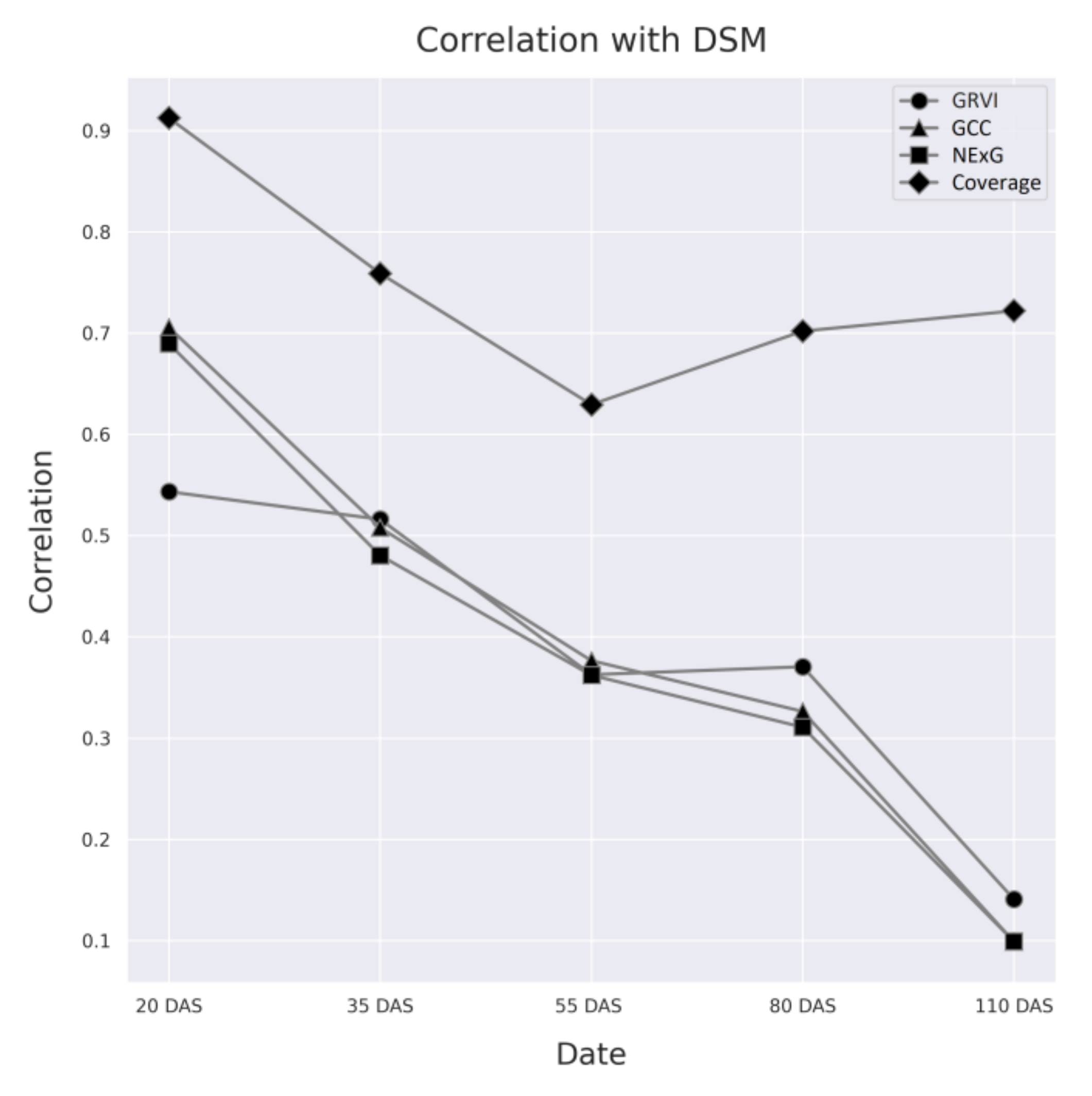
3.2. Correlation Analysis

The correlation between the data from VI and vegetation coverage and the respective DSM of each data collection date are shown in Table 4 and Figure 13 below. Among the VIs, GCC showed the highest correlation across the first three dates, followed by NExG, which also followed a similar pattern. Both indices exhibited the highest correlation with cotton height at the early stages and then steadily decreased as they approached the later stages of maturity. GRVI, on the other hand, had the lowest correlation early in the season, and although it mirrored a similar trend and dropped sharply at later stages, it slightly outperformed GCC and NExG at 80 and 110 DAS. Moreover, cotton vegetation coverage showed a more consistent trend throughout the season, beginning with a correlation above 91% in 20 DAS, when young cotton plants were easily distinguishable from the background.

4. Discussion

The results show that the proposed method is able to produce highly accurate DSMs of the experimental cotton field, which is also confirmed by the growth curve produced, as the results are consistent with the standard growth curve for cotton according to the agronomic literature [29]. Soil coverage of cotton foliage also showed a high correlation with vertical plant growth. The strongest correlation between vertical (plant height) and horizontal (vegetation coverage) cotton growth was observed at the earlier growth stages, possibly due to the fact that the younger plants are easier to separate from the background. In contrast, the lowest correlation was observed at the 3rd measurement when plants were near their maximum height for the current growing season.
Wu et al. [65] obtained comparable outcomes by constructing dense point clouds from UAS RGB images to assess cotton plant height and LAI after cotton defoliant spraying. Their method was able to dynamically monitor the changes in the LAI of cotton at different times (R2 and RMSE values for the estimated plant height based on the dense point cloud and the measured plant height were 0.962 and 0.913, respectively), leading to the conclusion that dense point cloud construction based on UAS remote sensing is a potential alternative to plant height and LAI estimation.
Phenotyping based on 3D models can play a significant role in improving the efficiency and productivity of the agriculture sector. By providing the ability to continuously monitor and quantify plant growth, as well as their responses to various abiotic stress factors, 3D models can assist growers in making informed decisions. In several studies, the use of 3D models for crop phenotyping has been found to be effective. For instance, in a study by Rose et al. [66], the growth of tomato plants was monitored using 3D point cloud technology, which showed a high correlation between the temporal leaf area index (LAI) and plant height (R2 > 0.96). Similar models were also developed for crops such as maize and sugar beets, which were found to have a good correlation with the yield [31]. In horticulture, the leaf area is considered a crucial factor in determining the growth capacity of a tree and, as a result, its yield [67]. Hence, LAI information may become crucial in adjusting the optimal number of fruit per tree in perennial crops using variable rate applications. Furthermore, recent advancements in 3D models have led to the development of methods to estimate structural parameters such as leaf area and chlorophyll content in broadleaf plants [68]. In a recent study by [69], the leaf area and fruit NDVI were estimated using 3D LiDAR data and were found to have a high correlation with reference data of fruit NDVI and chemically analyzed chlorophyll, with R2 values of 0.65 (RMSE = 0.65%) and 0.78 (RMSE = 1.31%), respectively. In conclusion, the use of 3D models for crop phenotyping has the potential to revolutionize the agriculture sector, providing growers with valuable information about their crops and enabling them to make informed decisions to improve productivity and efficiency.
By obtaining information on the different growth trends in different field zones and the overall spatial variability in the field, the methodology proposed in this article can help cotton producers to more effectively use agricultural inputs such as growth regulators and defoliants that are growth (and thus time) dependent. Barbedo et al. [70] and Ballester et al. [71] note in their research that younger plants have a higher biomass production rate compared to nitrogen accumulation (N dilution effect), which might explain this result. The lowest correlation, on the other hand, was seen at the third measurement, when the plants were approaching their maximum height for the current growing season. Lu et al. [14] in their study attempted to estimate maize plant height from the ideal percentile height of a point cloud and examine if the combination of plant height and canopy coverage with visible vegetation index might improve leaf nitrogen concentration (LNC) estimation accuracy. They discovered that the 99.9th percentile height of a point cloud was ideal for predicting plant height, implying that the combination of agronomy factors and VIs from UAS-based RGB photos had the ability to estimate LNC (which exhibited the highest correlation with maize at LNC = 0.716). The VIs used in this study were strongly correlated with plant height at the early growth stages, with satisfactory results from the GCC and NExG indices. These indices showed the highest correlation with cotton height at the early growth stages (between 60% and 70%).
More specifically, VIs followed a contiguous trend during the growing season, starting with low values at the beginning and increasing until the middle of the season, followed by a sharp decrease towards the end. The third index, GRVI, a widely used visible spectrum index VI, had the lowest correlation in the early growing stages, although its relative performance increased slightly in later stages, outperforming GCC and NExG. However, since the correlation with all VIs was low after 55 DAS, no clear conclusion can be drawn about the ability of VIs to estimate plant height at later growth stages when vegetation vigor is lower. This suggests that the proposed method is more accurate in estimating cotton height at early growth stages through photogrammetry, but may be less reliable at estimating crop height through VIs at later stages. In contrast, the most reliable method would be mapping at approximately 55 DAS to obtain information on field variability. Finally, the photogrammetric pipeline described in this study proved to be very accurate, as errors between ground truth measurements and generated DSM values were insignificant (consistently less than 5%).
Cotton vegetation cover showed a more consistent trend, with a correlation of over 91% in the early stages when young cotton plants were easily distinguishable from the background. The decrease in later stages may also be attributed to the presence of other vegetation in the field, such as weeds, which occurred in several field zones throughout the growing season. Similar issues caused by the presence of weeds have been highlighted in other research, such as [72], where the presence of weeds and fuzzy effects in the photos generated noise and led to inaccuracies. Overall, this study provides promising results for the potential of using visible spectrum reflectance data and photogrammetric DSM models to estimate cotton plant height, particularly in the early growth stages. Further research is needed to improve the accuracy of the method at later growth stages and explore its potential for use in other crop types and cultivation systems.

5. Conclusions

The present study has shown that the proposed methodology using visible spectrum reflectance data and photogrammetric DSM models can accurately estimate the vertical growth of cotton plants at the early growth stages. The GCC and NExG indices showed the most satisfactory results in this regard. However, the correlations between the different vegetation indices and vertical plant growth appeared to decrease as the growing season progressed. The GRVI index showed the lowest correlation in the early growth stages, although its performance improved slightly in later stages. However, it is unclear whether VIs can accurately estimate plant height at later growth stages when vegetation vigor is lower. The photogrammetric pipeline used in this study proved to be very accurate, with errors consistently below 5%. Because the overall correlation between data from VI and plant height showed significant temporal variation, it is recommended that the mapping of 50 DAS be conducted based on the results of this study to provide more reliable information about variability in the field. These results could be useful in developing more accurate models to predict cotton plant height and optimize land management strategies. Overall, this study provides a promising alternative method for estimating cotton plant height using low-cost UAS-derived spectral index information and photogrammetric modeling. These initial results suggest that the proposed method of using visible spectrum reflectance data and photogrammetric DSM models may be a useful tool for estimating cotton plant height at the early growth stages. Further research could improve the accuracy of the method at later growth stages and investigate its potential for use in other crops.

Author Contributions

Conceptualization, V.P., A.K. and S.F.; methodology, V.P. and N.T.; software, V.P. and N.T.; validation, V.P., A.K. and G.P.; formal analysis, V.P. and N.T.; investigation, V.P. and A.K.; resources, S.F.; data curation, V.P. and G.P.; writing—original draft preparation, V.P.; writing—review and editing, A.K. and G.P.; visualization, V.P.; supervision, S.F.; project administration, V.P. All authors have read and agreed to the published version of the manuscript.

Funding

This research received no external funding.

Data Availability Statement

The data presented in this study are available upon request from the corresponding author. The data are not publicly available due to the privacy of the data collection location.

Conflicts of Interest

The authors declare no conflict of interest.

References

  1. Jiang, Y.; Li, C.; Paterson, A.H.; Sun, S.; Xu, R.; Robertson, J. Quantitative Analysis of Cotton Canopy Size in Field Conditions Using a Consumer-Grade RGB-D Camera. Front. Plant Sci. 2018, 8, 2233. [Google Scholar] [CrossRef] [Green Version]
  2. Sun, S.; Li, C.; Paterson, A.; Jiang, Y.; Robertson, J. 3D Computer Vision and Machine Learning Based Technique for High Throughput Cotton Boll Mapping under Field Conditions. In Proceedings of the 2018 ASABE Annual International Meeting, Detroit, MI, USA, 29 July–1 August 2018; American Society of Agricultural and Biological Engineers: St. Joseph, MI, USA, 2018. [Google Scholar]
  3. Feng, A.; Zhou, J.; Vories, E.D.; Sudduth, K.A.; Zhang, M. Yield Estimation in Cotton Using UAV-Based Multi-Sensor Imagery. Biosyst. Eng. 2020, 193, 101–114. [Google Scholar] [CrossRef]
  4. Johnson, R.M.; Downer, R.G.; Bradow, J.M.; Bauer, P.J.; Sadler, E.J. Variability in Cotton Fiber Yield, Fiber Quality, and Soil Properties in a Southeastern Coastal Plain. Agron. J. 2002, 94, 1305–1316. [Google Scholar] [CrossRef] [Green Version]
  5. Zhang, J.; Fang, H.; Zhou, H.; Sanogo, S.; Ma, Z. Genetics, Breeding, and Marker-Assisted Selection for Verticillium Wilt Resistance in Cotton. Crop Sci. 2014, 54, 1289–1303. [Google Scholar] [CrossRef]
  6. Phillips, R.L. Mobilizing Science to Break Yield Barriers. Crop Sci. 2010, 50, S-99–S-108. [Google Scholar] [CrossRef] [Green Version]
  7. Thompson, A.; Thorp, K.; Conley, M.; Elshikha, D.; French, A.; Andrade-Sanchez, P.; Pauli, D. Comparing Nadir and Multi-Angle View Sensor Technologies for Measuring in-Field Plant Height of Upland Cotton. Remote Sens. 2019, 11, 700. [Google Scholar] [CrossRef] [Green Version]
  8. Ashapure, A.; Jung, J.; Chang, A.; Oh, S.; Maeda, M.; Landivar, J. A Comparative Study of RGB and Multispectral Sensor-Based Cotton Canopy Cover Modelling Using Multi-Temporal UAS Data. Remote Sens. 2019, 11, 2757. [Google Scholar] [CrossRef] [Green Version]
  9. Goggin, F.L.; Lorence, A.; Topp, C.N. Applying High-Throughput Phenotyping to Plant–Insect Interactions: Picturing More Resistant Crops. Curr. Opin. Insect Sci. 2015, 9, 69–76. [Google Scholar] [CrossRef] [Green Version]
  10. Großkinsky, D.K.; Pieruschka, R.; Svensgaard, J.; Rascher, U.; Christensen, S.; Schurr, U.; Roitsch, T. Phenotyping in the Fields: Dissecting the Genetics of Quantitative Traits and Digital Farming. New Phytol. 2015, 207, 950–952. [Google Scholar] [CrossRef]
  11. Rahaman, M.M.; Chen, D.; Gillani, Z.; Klukas, C.; Chen, M. Advanced Phenotyping and Phenotype Data Analysis for the Study of Plant Growth and Development. Front. Plant Sci. 2015, 6, 619. [Google Scholar] [CrossRef] [Green Version]
  12. Sun, S.; Li, C.; Paterson, A. In-Field High-Throughput Phenotyping of Cotton Plant Height Using LiDAR. Remote Sens. 2017, 9, 377. [Google Scholar] [CrossRef] [Green Version]
  13. Chu, T.; Chen, R.; Landivar, J.A.; Maeda, M.M.; Yang, C.; Starek, M.J. Cotton Growth Modeling and Assessment Using Unmanned Aircraft System Visual-Band Imagery. J. Appl. Remote Sens. 2016, 10, 036018. [Google Scholar] [CrossRef] [Green Version]
  14. Lu, J.; Cheng, D.; Geng, C.; Zhang, Z.; Xiang, Y.; Hu, T. Combining Plant Height, Canopy Coverage and Vegetation Index from UAV-Based RGB Images to Estimate Leaf Nitrogen Concentration of Summer Maize. Biosyst. Eng. 2021, 202, 42–54. [Google Scholar] [CrossRef]
  15. Richardson, C.W. Weather Simulation for Crop Management Models. Trans. ASAE 1985, 28, 1602–1606. [Google Scholar] [CrossRef]
  16. Wilkerson, G.G.; Jones, J.W.; Boote, K.J.; Ingram, K.T.; Mishoe, J.W. Modeling Soybean Growth for Crop Management. Trans. ASAE 1983, 26, 63–73. [Google Scholar] [CrossRef]
  17. Pabuayon, I.L.B.; Sun, Y.; Guo, W.; Ritchie, G.L. High-Throughput Phenotyping in Cotton: A Review. J. Cotton Res. 2019, 2, 18. [Google Scholar] [CrossRef]
  18. Thapa, S.; Zhu, F.; Walia, H.; Yu, H.; Ge, Y. A Novel LiDAR-Based Instrument for High-Throughput, 3D Measurement of Morphological Traits in Maize and Sorghum. Sensors 2018, 18, 1187. [Google Scholar] [CrossRef] [Green Version]
  19. Yin, X.; McClure, M.A. Relationship of Corn Yield, Biomass, and Leaf Nitrogen with Normalized Difference Vegetation Index and Plant Height. Agron. J. 2013, 105, 1005–1016. [Google Scholar] [CrossRef]
  20. Zarco-Tejada, P.J.; Diaz-Varela, R.; Angileri, V.; Loudjani, P. Tree Height Quantification Using Very High Resolution Imagery Acquired from an Unmanned Aerial Vehicle (UAV) and Automatic 3D Photo-Reconstruction Methods. Eur. J. Agron. 2014, 55, 89–99. [Google Scholar] [CrossRef]
  21. Murchie, E.H.; Pinto, M.; Horton, P. Agriculture and the New Challenges for Photosynthesis Research. New Phytol. 2009, 181, 532–552. [Google Scholar] [CrossRef]
  22. Reta-Sánchez, D.G.; Fowler, J.L. Canopy Light Environment and Yield of Narrow-Row Cotton as Affected by Canopy Architecture. Agron. J. 2002, 94, 1317–1323. [Google Scholar] [CrossRef]
  23. Zhu, X.-G.; Long, S.P.; Ort, D.R. Improving Photosynthetic Efficiency for Greater Yield. Annu. Rev. Plant Biol. 2010, 61, 235–261. [Google Scholar] [CrossRef] [Green Version]
  24. Stamatiadis, S.; Tsadilas, C.; Schepers, J.S. Ground-Based Canopy Sensing for Detecting Effects of Water Stress in Cotton. Plant Soil 2010, 331, 277–287. [Google Scholar] [CrossRef]
  25. Tilly, N.; Hoffmeister, D.; Cao, Q.; Huang, S.; Lenz-Wiedemann, V.; Miao, Y.; Bareth, G. Multitemporal Crop Surface Models: Accurate Plant Height Measurement and Biomass Estimation with Terrestrial Laser Scanning in Paddy Rice. J. Appl. Remote Sens. 2014, 8, 083671. [Google Scholar] [CrossRef]
  26. Oosterhuis, D.M. Growth and Development of a Cotton Plant. In Nitrogen Nutrition of Cotton: Practical Issues; Miley, W.N., Oosterhuis, D.M., Eds.; ASA, CSSA, and SSSA Books; American Society of Agronomy: Madison, WI, USA, 2015; pp. 1–24. ISBN 978-0-89118-244-3. [Google Scholar]
  27. Liu, K.; Dong, X.; Qiu, B. Analysis of Cotton Height Spatial Variability Based on UAV-LiDAR. Int. J. Precis. Agric. Aviat. 2018, 1, 72–76. [Google Scholar] [CrossRef]
  28. Sui, R.; Fisher, D.K.; Reddy, K.N. Cotton Yield Assessment Using Plant Height Mapping System. J. Agric. Sci. 2012, 5, 23. [Google Scholar] [CrossRef] [Green Version]
  29. Oosterhuis, D.M.; Kosmidou, K.K.; Cothren, J.T. Managing Cotton Growth and Development with Plant Growth Regulators. In Proceedings of the World Cotton Research Conference-2, Athens, Greece, 6–12 September 1998; pp. 6–12. [Google Scholar]
  30. Sanz, R.; Rosell, J.R.; Llorens, J.; Gil, E.; Planas, S. Relationship between Tree Row LIDAR-Volume and Leaf Area Density for Fruit Orchards and Vineyards Obtained with a LIDAR 3D Dynamic Measurement System. Agric. For. Meteorol. 2013, 171–172, 153–162. [Google Scholar] [CrossRef] [Green Version]
  31. Martinez-Guanter, J.; Ribeiro, Á.; Peteinatos, G.G.; Pérez-Ruiz, M.; Gerhards, R.; Bengochea-Guevara, J.M.; Machleb, J.; Andújar, D. Low-Cost Three-Dimensional Modeling of Crop Plants. Sensors 2019, 19, 2883. [Google Scholar] [CrossRef] [Green Version]
  32. Barker, J.; Zhang, N.; Sharon, J.; Steeves, R.; Wang, X.; Wei, Y.; Poland, J. Development of a Field-Based High-Throughput Mobile Phenotyping Platform. Comput. Electron. Agric. 2016, 122, 74–85. [Google Scholar] [CrossRef] [Green Version]
  33. Sharma, B.; Ritchie, G.L. High-Throughput Phenotyping of Cotton in Multiple Irrigation Environments. Crop Sci. 2015, 55, 958–969. [Google Scholar] [CrossRef] [Green Version]
  34. Araus, J.L.; Cairns, J.E. Field High-Throughput Phenotyping: The New Crop Breeding Frontier. Trends Plant Sci. 2014, 19, 52–61. [Google Scholar] [CrossRef]
  35. Barabaschi, D.; Tondelli, A.; Desiderio, F.; Volante, A.; Vaccino, P.; Valè, G.; Cattivelli, L. Next Generation Breeding. Plant Sci. 2016, 242, 3–13. [Google Scholar] [CrossRef]
  36. Cobb, J.N.; DeClerck, G.; Greenberg, A.; Clark, R.; McCouch, S. Next-Generation Phenotyping: Requirements and Strategies for Enhancing Our Understanding of Genotype–Phenotype Relationships and Its Relevance to Crop Improvement. Appl. Genet. 2013, 126, 867–887. [Google Scholar] [CrossRef] [Green Version]
  37. White, J.W.; Andrade-Sanchez, P.; Gore, M.A.; Bronson, K.F.; Coffelt, T.A.; Conley, M.M.; Feldmann, K.A.; French, A.N.; Heun, J.T.; Hunsaker, D.J.; et al. Field-Based Phenomics for Plant Genetics Research. Field Crops Res. 2012, 133, 101–112. [Google Scholar] [CrossRef]
  38. Xu, R.; Li, C.; Paterson, A.H. Multispectral Imaging and Unmanned Aerial Systems for Cotton Plant Phenotyping. PLoS ONE 2019, 14, e0205083. [Google Scholar] [CrossRef] [Green Version]
  39. Miao, T.; Zhu, C.; Xu, T.; Yang, T.; Li, N.; Zhou, Y.; Deng, H. Automatic Stem-Leaf Segmentation of Maize Shoots Using Three-Dimensional Point Cloud. Comput. Electron. Agric. 2021, 187, 106310. [Google Scholar] [CrossRef]
  40. Campos, J.; García-Ruíz, F.; Gil, E. Assessment of Vineyard Canopy Characteristics from Vigour Maps Obtained Using UAV and Satellite Imagery. Sensors 2021, 21, 2363. [Google Scholar] [CrossRef]
  41. Comba, L.; Biglia, A.; Ricauda Aimonino, D.; Tortia, C.; Mania, E.; Guidoni, S.; Gay, P. Leaf Area Index Evaluation in Vineyards Using 3D Point Clouds from UAV Imagery. Precis. Agric. 2020, 21, 881–896. [Google Scholar] [CrossRef] [Green Version]
  42. Tao, H.; Feng, H.; Xu, L.; Miao, M.; Long, H.; Yue, J.; Li, Z.; Yang, G.; Yang, X.; Fan, L. Estimation of Crop Growth Parameters Using UAV-Based Hyperspectral Remote Sensing Data. Sensors 2020, 20, 1296. [Google Scholar] [CrossRef] [Green Version]
  43. Tsouros, D.C.; Bibi, S.; Sarigiannidis, P.G. A Review on UAV-Based Applications for Precision Agriculture. Information 2019, 10, 349. [Google Scholar] [CrossRef] [Green Version]
  44. Roth, L.; Streit, B. Predicting Cover Crop Biomass by Lightweight UAS-Based RGB and NIR Photography: An Applied Photogrammetric Approach. Precis. Agric. 2018, 19, 93–114. [Google Scholar] [CrossRef] [Green Version]
  45. Singh, K.K.; Frazier, A.E. A Meta-Analysis and Review of Unmanned Aircraft System (UAS) Imagery for Terrestrial Applications. Int. J. Remote Sens. 2018, 39, 5078–5098. [Google Scholar] [CrossRef]
  46. Chang, A.; Jung, J.; Maeda, M.M.; Landivar, J. Crop Height Monitoring with Digital Imagery from Unmanned Aerial System (UAS). Comput. Electron. Agric. 2017, 141, 232–237. [Google Scholar] [CrossRef]
  47. Yeom, J.; Jung, J.; Chang, A.; Ashapure, A.; Maeda, M.; Maeda, A.; Landivar, J. Comparison of Vegetation Indices Derived from UAV Data for Differentiation of Tillage Effects in Agriculture. Remote Sens. 2019, 11, 1548. [Google Scholar] [CrossRef] [Green Version]
  48. Jung, J.; Maeda, M.; Chang, A.; Landivar, J.; Yeom, J.; McGinty, J. Unmanned Aerial System Assisted Framework for the Selection of High Yielding Cotton Genotypes. Comput. Electron. Agric. 2018, 152, 74–81. [Google Scholar] [CrossRef]
  49. Bendig, J.; Bolten, A.; Bareth, G. 4 UAV-based Imaging for Multi-Temporal, very high Resolution Crop Surface Models to monitor Crop Growth Variability. In Unmanned Aerial Vehicles (UAVs) for Multi-Temporal Crop Surface Modelling; Universität zu Köln: Cologne, Germany, 2013; pp. 44–60. [Google Scholar] [CrossRef]
  50. Chang, A.; Jung, J.; Yeom, J.; Landivar, J. 3D Characterization of Sorghum Panicles Using a 3D Point Cloud Derived from UAV Imagery. Remote Sens. 2021, 13, 282. [Google Scholar] [CrossRef]
  51. Chen, R.; Chu, T.; Landivar, J.A.; Yang, C.; Maeda, M.M. Monitoring Cotton (Gossypium hirsutum L.) Germination Using Ultrahigh-Resolution UAS Images. Precis. Agric. 2018, 19, 161–177. [Google Scholar] [CrossRef]
  52. Chu, T.; Starek, M.J.; Brewer, M.J.; Murray, S.C.; Pruter, L.S. Characterizing Canopy Height with UAS Structure-from-Motion Photogrammetry—Results Analysis of a Maize Field Trial with Respect to Multiple Factors. Remote Sens. Lett. 2018, 9, 753–762. [Google Scholar] [CrossRef] [Green Version]
  53. Grenzdörffer, G.J. Crop Height Determination with UAS Point Clouds. Int. Arch. Photogramm. Remote Sens. Spat. Inf. Sci. 2014, XL-1, 135–140. [Google Scholar] [CrossRef] [Green Version]
  54. Stanton, C.; Starek, M.J.; Elliott, N.; Brewer, M.; Maeda, M.M.; Chu, T. Unmanned Aircraft System-Derived Crop Height and Normalized Difference Vegetation Index Metrics for Sorghum Yield and Aphid Stress Assessment. J. Appl. Remote Sens. 2017, 11, 026035. [Google Scholar] [CrossRef] [Green Version]
  55. Torres-Sánchez, J.; López-Granados, F.; Serrano, N.; Arquero, O.; Peña, J.M. High-Throughput 3-D Monitoring of Agricultural-Tree Plantations with Unmanned Aerial Vehicle (UAV) Technology. PLoS ONE 2015, 10, e0130479. [Google Scholar] [CrossRef] [Green Version]
  56. Westoby, M.J.; Brasington, J.; Glasser, N.F.; Hambrey, M.J.; Reynolds, J.M. ‘Structure-from-Motion’ Photogrammetry: A Low-Cost, Effective Tool for Geoscience Applications. Geomorphology 2012, 179, 300–314. [Google Scholar] [CrossRef] [Green Version]
  57. Hoffmeister, D.; Bolten, A.; Curdt, C.; Waldhoff, G.; Bareth, G. High-Resolution Crop Surface Models (CSM) and Crop Volume Models (CVM) on Field Level by Terrestrial Laser Scanning. Proc. SPIE 2010, 7840, 78400E. [Google Scholar]
  58. Sassu, A.; Ghiani, L.; Salvati, L.; Mercenaro, L.; Deidda, A.; Gambella, F. Integrating UAVs and Canopy Height Models in Vineyard Management: A Time-Space Approach. Remote Sens. 2021, 14, 130. [Google Scholar] [CrossRef]
  59. Ashapure, A.; Jung, J.; Yeom, J.; Chang, A.; Maeda, M.; Maeda, A.; Landivar, J. A Novel Framework to Detect Conventional Tillage and No-Tillage Cropping System Effect on Cotton Growth and Development Using Multi-Temporal UAS Data. ISPRS J. Photogramm. Remote Sens. 2019, 152, 49–64. [Google Scholar] [CrossRef]
  60. Bendig, J.; Yu, K.; Aasen, H.; Bolten, A.; Bennertz, S.; Broscheit, J.; Gnyp, M.L.; Bareth, G. Combining UAV-Based Plant Height from Crop Surface Models, Visible, and near Infrared Vegetation Indices for Biomass Monitoring in Barley. Int. J. Appl. Earth Obs. Geoinf. 2015, 39, 79–87. [Google Scholar] [CrossRef]
  61. Díaz-Varela, R.; de la Rosa, R.; León, L.; Zarco-Tejada, P. High-Resolution Airborne UAV Imagery to Assess Olive Tree Crown Parameters Using 3D Photo Reconstruction: Application in Breeding Trials. Remote Sens. 2015, 7, 4213–4232. [Google Scholar] [CrossRef] [Green Version]
  62. Tucker, C.J. Red and photographic infrared linear combinations for monitoring vegetation. Remote Sens. Environ. 1979, 8, 127–150. [Google Scholar] [CrossRef] [Green Version]
  63. Nijland, W.; De Jong, R.; De Jong, S.M.; Wulder, M.A.; Bater, C.W.; Coops, N.C. Monitoring plant condition and phenology using infrared sensitive consumer grade digital cameras. Agric. For. Meteorol. 2014, 184, 98–106. [Google Scholar] [CrossRef] [Green Version]
  64. Woebbecke, D.M.; Meyer, G.E.; Von Bargen, K.; Mortensen, D.A. Plant species identification, size, and enumeration using machine vision techniques on near-binary images. Opt. Agric. For. 1993, 1836, 208–219. [Google Scholar]
  65. Wu, J.; Wen, S.; Lan, Y.; Yin, X.; Zhang, J.; Ge, Y. Estimation of cotton canopy parameters based on unmanned aerial vehicle (UAV) oblique photography. Plant Methods 2022, 18, 129. [Google Scholar] [CrossRef]
  66. Rose, J.C.; Paulus, S.; Kuhlmann, H. Accuracy analysis of a multi-view stereo approach for phenotyping of tomato plants at the organ level. Sensors 2015, 15, 9651–9665. [Google Scholar] [CrossRef] [Green Version]
  67. Penzel, M.; Herppich, W.B.; Weltzien, C.; Tsoulias, N.; Zude-Sasse, M. Modelling the tree-individual fruit bearing capacity aimed at optimising fruit quality of Malus domestica BORKH. ‘Brookfield Gala’. Front. Plant Sci. 2021, 13, 669909. [Google Scholar] [CrossRef]
  68. Eitel, J.U.; Vierling, L.A.; Long, D.S. Simultaneous measurements of plant structure and chlorophyll content in broadleaf saplings with a terrestrial laser scanner. Remote Sens. Environ. 2010, 114, 2229–2237. [Google Scholar] [CrossRef]
  69. Tsoulias, N.; Saha, K.K.; Zude-Sasse, M. In-situ fruit analysis by means of LiDAR 3D point cloud of normalized difference vegetation index (NDVI). Comput. Electron. Agric. 2023, 205, 107611. [Google Scholar] [CrossRef]
  70. Barbedo, J.G.A. A review on the use of unmanned aerial vehicles and imaging sensors for monitoring and assessing plant stresses. Drones 2019, 3, 40. [Google Scholar] [CrossRef] [Green Version]
  71. Ballester, C.; Hornbuckle, J.; Brinkhoff, J.; Smith, J.; Quayle, W. Assessment of in-season cotton nitrogen status and lint yield prediction from unmanned aerial system imagery. Remote Sens. 2017, 9, 1149. [Google Scholar] [CrossRef] [Green Version]
  72. García-Martínez, H.; Flores-Magdaleno, H.; Khalil-Gardezi, A.; Ascencio-Hernández, R.; Tijerina-Chávez, L.; Vázquez-Peña, M.A.; Mancilla-Villa, O.R. Digital count of corn plants using images taken by unmanned aerial vehicles and cross correlation of templates. Agronomy 2020, 10, 469. [Google Scholar] [CrossRef] [Green Version]
Figure 1. The relative location of the experimental area for this study, located in Aliartos, Greece. The geographical coordinates of the area are 38°23′40″N, 23°6′10″E, and the elevation is 265 m above sea level (ASL).
Remotesensing 15 01214 g001
Figure 2. The experimental area for this study was located in Aliartos, Greece.
Remotesensing 15 01214 g002
Figure 3. The UAS (a) that collected the RGB imagery and the RTK GPS (b) used to measure GCPs in this study.
Remotesensing 15 01214 g003
Figure 4. A segment from an RGB orthomosaic shows the elements that remain after the soil removal, namely cotton vegetation. The use of aerial imagery and digital filters enabled the isolation of the vegetation pixels from all other elements in the image, providing a more accurate and detailed picture of the ground cover.
Remotesensing 15 01214 g004
Figure 5. The data processing pipeline for the generation of the primary datasets of this study.
Remotesensing 15 01214 g005
Figure 6. The collection of the ground truth cotton height measurements.
Remotesensing 15 01214 g006
Figure 7. The distribution of the three (3) vegetation index values for the 1st measurement (20 DAS), shown in a histogram in relation to the corresponding DSM values.
Remotesensing 15 01214 g007
Figure 8. The distribution of the three (3) vegetation index values for the 2nd measurement (35 DAS), shown in a histogram in relation to the corresponding DSM values.
Remotesensing 15 01214 g008
Figure 9. The distribution of the three (3) vegetation index values for the 3rd measurement (55 DAS), shown in a histogram in relation to the corresponding DSM values.
Remotesensing 15 01214 g009
Figure 10. The distribution of the three (3) vegetation index values for the 4th measurement (80 DAS), shown in a histogram in relation to the corresponding DSM values.
Remotesensing 15 01214 g010
Figure 11. The distribution of the three (3) vegetation index values for the 5th measurement (110 DAS) shown in a histogram in relation to the corresponding DSM values.
Remotesensing 15 01214 g011
Figure 12. The VI values (a) and cotton horizontal growth curve (DSM values) (b) throughout the study.
Remotesensing 15 01214 g012
Figure 13. The correlation between DSM values and the three (3) Vis used in this study, across all data collection dates.
Remotesensing 15 01214 g013
Table 1. The VIs used in this study with their respective spectral equations. These VIs were calculated using their respective spectral equations, by using red, green, and blue reflectance values recorded by the RGB sensor of the UAS. By applying these equations to the aerial imagery, it is possible to obtain information regarding the plant’s health status, such as chlorophyll content and leaf area index.
Vegetation IndexSpectral Expression
Green-Red Vegetation Index (GRVI) [62](Green − Red)/(Green + Red)
Green Chromatic Coordinate Index (GCC) [63](Green)/(Green + Red + Blue)
Normalized Excessive Green Index (NExG) [64](2 × Green − Red − Blue)/(Green + Red + Blue)
Table 2. The average VI and DSM values for all measurements at the resolution of the reference grid (10 × 10 m2).
DateGRVIGCCNExGDSM
20 DAS0.1008140.3974830.2013970.391097
35 DAS0.1311250.4116990.2412740.596634
55 DAS0.1977060.448510.349080.763857
80 DAS0.0996960.393780.1862770.678612
110 DAS0.0358440.37440.1231990.651831
Table 3. The value ranges for all three (3) VIs and DSM values across the five (5) data collection dates at the resolution of the reference grid (10 × 10 m2).
DateGRVIGCCNExGDSM
20 DAS0.026–0.1610.368–0.4210.120–0.2670.200–0.573
35 DAS0.049–0.1760.382–0.4290.160–0.2940.253–0.78
55 DAS0.060–0.2640.385–0.4870.171–0.4630.282–1.02
80 DAS0.028–0.2080.370–0.4420.121–0.3260.388–1.07
110 DAS0.018–0.0790.368–0.3890.105–0.1680.390–1.084
Table 4. The Pearson correlation values between VI data and canopy coverage and the respective DSMs at the resolution of the reference grid (10 × 10 m2).
DateGRVIGCCNExGCoverage
20 DAS0.5430.7060.6090.913
35 DAS0.5160.5080.4810.759
55 DAS0.3630.3770.3620.630
80 DAS0.3710.3260.3110.702
110 DAS0.1410.0990.0990.722
Disclaimer/Publisher’s Note: The statements, opinions and data contained in all publications are solely those of the individual author(s) and contributor(s) and not of MDPI and/or the editor(s). MDPI and/or the editor(s) disclaim responsibility for any injury to people or property resulting from any ideas, methods, instructions or products referred to in the content.

