Communication

Which Vegetation Index? Benchmarking Multispectral Metrics to Hyperspectral Mixture Models in Diverse Cropland

1
Department of Geography, San Diego State University, San Diego, CA 92182, USA
2
Lamont-Doherty Earth Observatory, Columbia University, New York, NY 10964, USA
*
Author to whom correspondence should be addressed.
Remote Sens. 2023, 15(4), 971; https://doi.org/10.3390/rs15040971
Submission received: 31 December 2022 / Revised: 1 February 2023 / Accepted: 5 February 2023 / Published: 10 February 2023

Abstract

:
The monitoring of agronomic parameters like biomass, water stress, and plant health can benefit from synergistic use of all available remotely sensed information. Multispectral imagery has been used for this purpose for decades, largely with vegetation indices (VIs). Many multispectral VIs exist, typically relying on a single feature—the spectral red edge—for information. Where hyperspectral imagery is available, spectral mixture models can use the full VSWIR spectrum to yield further insight, simultaneously estimating area fractions of multiple materials within mixed pixels. Here we investigate the relationships between VIs and mixture models by comparing hyperspectral endmember fractions to six common multispectral VIs in California’s diverse crops and soils. In so doing, we isolate spectral effects from sensor- and acquisition-specific variability associated with atmosphere, illumination, and view geometry. Specifically, we compare: (1) fractional area of photosynthetic vegetation (Fv) from 64,000,000 3–5 m resolution AVIRIS-ng reflectance spectra; and (2) six popular VIs (NDVI, NIRv, EVI, EVI2, SR, DVI) computed from simulated Planet SuperDove reflectance spectra derived from the AVIRIS-ng spectra. Hyperspectral Fv and multispectral VIs are compared using both parametric (Pearson correlation, ρ) and nonparametric (Mutual Information, MI) metrics. Four VIs (NIRv, DVI, EVI, EVI2) showed strong linear relationships with Fv (ρ > 0.94; MI > 1.2). NIRv and DVI showed strong interrelation (ρ > 0.99, MI > 2.4), but deviated from a 1:1 correspondence with Fv. EVI and EVI2 were strongly interrelated (ρ > 0.99, MI > 2.3) and more closely approximated a 1:1 relationship with Fv. In contrast, NDVI and SR showed a weaker, nonlinear, heteroskedastic relation to Fv (ρ < 0.84, MI = 0.69). NDVI exhibited both especially severe sensitivity to unvegetated background (–0.05 < NDVI < +0.6) and saturation (0.2 < Fv < 0.8 for NDVI = 0.7). The self-consistent atmospheric correction, radiometry, and sun-sensor geometry allows this simulation approach to be further applied to indices, sensors, and landscapes worldwide.

1. Introduction

Agricultural remote sensing is undergoing a fundamental transformation. On the one hand, imaging spectroscopy (hyperspectral) missions such as SBG, EMIT, EnMAP, DESIS, PRISMA, and HISUI [1,2,3,4,5] promise more accurate plant phenotyping, including measures of important concerns such as water stress and nutrient deficiency [6] by improving spectral fidelity. Simultaneously, CubeSat constellations such as Planet enable order-of-magnitude improvements in spatial and temporal resolution of multispectral satellite imagery [7], allowing for improved intra-field monitoring — if radiometric inconsistencies can be overcome [8]. As the volume and variety of optical imagery continue to accelerate, applications will demand models capable of the synergistic use of datasets with widely varying spatial, spectral, and temporal resolutions and noise characteristics. Developing such models will thus require a quantitative understanding of the relationships between metrics derived from various sensors, in order to best leverage the strengths and mitigate the limitations of each.
Agricultural applications have been a primary focus of optical remote sensing since the inception of the field, and spectral vegetation indices (VIs) have for decades been one of the most commonly used tools for this purpose [9,10]. Over the decades, computational simplicity and ease of use have resulted in a proliferation of VI options (e.g., [11,12,13,14,15]). The growing availability and diminishing cost of decameter [16,17] and sub-decameter [18] multispectral satellite imagery is making VIs increasingly popular with a broader science and applications community. Data from Planet’s Dove and SuperDove sensors are of particular interest given their (nominal) daily global coverage and 3–4.2 m spatial resolution [7], with constantly improving utility for agricultural land management [19]. Such applications span a broad range, including high resolution soil moisture mapping [20], leaf area index [21], pest impacts [22], crop maturation [23], and more.
As recently reviewed by [24,25,26], popular multispectral VIs vary widely in underlying theoretical basis and conceptual interrelationships. Yet despite this complexity, independent evaluations of multispectral VIs against other approaches for vegetation abundance estimation, particularly using hyperspectral data, are relatively rare. These comparisons will be critical given the proliferation of spaceborne hyperspectral data that is planned for the coming decade. Here, we leveraged existing, state-of-the-art airborne hyperspectral imagery to conduct such a comparative analysis for six popular vegetation indices over a diverse, globally significant agricultural landscape.
Global compilations of multispectral imagery from spectrally diverse landscapes have compared and contrasted interrelationships among vegetation indices through the use of bivariate distributions between pairs of indices (e.g., [27]). Results of these intercomparisons have shown a wide range of interrelationships among vegetation indices often assumed to be interchangeable metrics for the same physical quantity—green vegetation cover at pixel scale. However, these studies have generally relied on decameter (or hectometer) resolution multispectral imagery, which is known to alias spectral signatures and introduce varying degrees of linear and nonlinear spectral mixing within sensor ground-projected instantaneous fields of view (IFOVs) at these scales. In addition, global compilations of top-of-atmosphere reflectance spectra generally incorporate a variety of atmospheric and bidirectional reflectance distribution function (BRDF) effects.
We sought to minimize distortions arising from spatial and spectral aliasing, as well as atmospheric and BRDF effects, by using a compilation of 64,000,000 high quality Airborne Visible/Infrared Imaging Spectrometer Next Generation (AVIRIS-ng) hyperspectra from a diversity of agricultural landscapes in California to quantify characteristics of six widely used broadband vegetation indices. Here we used spatially and spectrally oversampled reflectances, derived from a state-of-the-art imaging spectrometer and atmospherically corrected with a state-of-the-art radiative transfer model. Simulating multispectral data directly from these observations minimizes the biases inherent in using compilations of broadband data and allows simultaneous quantitative intercomparison of tens of millions of reflectance spectra from a diversity of substrates and vegetation.
Here, we compiled 64,000,000 5 nm, 3–5 m, AVIRIS-ng reflectance spectra from 15 flight lines collected throughout California in 2020. We estimated the photosynthetic vegetation fraction (Fv), as well as the substrate and shadow fractions, from each AVIRIS spectrum by inverting a three-endmember linear spectral mixture model. We then convolved each 425-band AVIRIS reflectance spectrum with the 8-band spectral response of the Planet SuperDove sensor and used these simulated SuperDove spectra to compute VIs for each spectrum. We quantified the relationship of each VI distribution relative to the hyperspectral Fv distribution for the full set of mixed spectra.
In so doing, we addressed the following questions:
  • How do the linearity and dispersion of each VI distribution vary with photosynthetic vegetation fraction estimated by the spectral mixture model?
  • How sensitive is each multispectral VI to substrate background from common agricultural materials like soil, rock, non-photosynthetic vegetation, or plastics?
  • How does a traditional parametric similarity metric (Pearson correlation, ρ) compare to a popular nonparametric metric (Mutual Information, MI) for such a comparison?

2. Materials and Methods

This study relied upon 15 flight lines collected in late summer of 2020 with the Advanced Visible Infrared Imaging Spectrometer-Next Generation (AVIRIS-ng) instrument. AVIRIS-ng measures radiance from 380 to 2510 nm at 5 nm intervals [28]. All flight lines were downloaded from the AVIRIS-ng data portal (https://avirisng.jpl.nasa.gov/dataportal, accessed on 1 June 2022) as orthorectified radiance. Each line was converted to surface reflectance using the Imaging Spectrometer Optimal FITting algorithm (ISOFIT) [29]. ISOFIT version 2.9.2 was used, as cloned from https://github.com/isofit/isofit (accessed on 1 June 2022). For all ISOFIT runs, the empirical line method flag was turned on (ELM = 1), with segmentation size = 200.
After atmospheric correction, reflectance data in wavelength ranges 376–421, 1123–1173, 1323–1498, 1774–2024, and 2450–2500 nm (AVIRIS-ng bands 1–10, 150–160, 190–225, 280–330, 415–425) were excluded from statistical analyses due to atmospheric contamination, resulting in the retention of 306 of 425 bands. Several 600 × 800-pixel subsets were extracted from each flightline and mosaiced into a single composite image cube of 64,000,000 pixel spectra.
All lines were flown in California between 24 July and 24 September 2020 (Figure 1). Flight altitude for all lines was approximately 10,300 ft (3140 m), resulting in a ground sampling distance of roughly 3 m. The lines sampled broad crop and soil diversity within one of the most productive agricultural landscapes on Earth [30]. Flights spanned a broad diversity of soils [31] hosting orchards, vineyards, and row crops, as well as some native and suburban vegetation. Nearly all agriculture in the study area is irrigated and planted/harvested asynchronously, resulting in a wide range of soil exposure, moisture content, growth stage, and canopy closure within each line.
This study focuses on the question of sensor interoperability. Specifically, we seek to isolate the subset of interoperability which is fundamentally spectral from platform- or acquisition-specific factors such as view and illumination geometry, ground sampling distance, second-to-minute scale atmospheric variability, or sensor radiometric calibration. Here, we control for these factors by directly simulating Planet data by convolving the AVIRIS-ng surface reflectance with the spectral response of the SuperDove sensor obtained from: https://developers.planet.com/docs/apis/data/sensors/ (accessed on 1 June 2022). A total of 6 indices were chosen on the basis of their popularity, as recently reviewed by [26]. The indices used in this study are: Difference Vegetation Index (DVI, [32]), Simple Ratio (SR [10], scaled by 0.1), Normalized Difference Vegetation Index (NDVI [11]), Near-Infrared Reflectance of Vegetation (NIRv [15]), Enhanced Vegetation Index (EVI [13]), and two-band Enhanced Vegetation Index (EVI2 [14]). Formulas for each index are given in Table 1.
Similarity metrics were computed in Python. Pearson correlation coefficients (ρ) were computed using NumPy v1.21.2 (numpy.corrcoef). Mutual information (MI) was computed using scikit-learn v0.24.2 (sklearn.feature_selection.mutual_info_regression). MI uses the Kullback–Leibler divergence of the marginal distributions of two variables to quantify the amount of information that can be obtained about one variable by observing the other variable [33,34,35,36]. Unlike ρ, MI does not require parametric statistical assumptions (or even real-valued variables), so should provide a more accurate estimate of the strength of non-Gaussian and nonlinear relationships.
A linear regression estimation for the NIRv:Fv was conducted in the R computing environment (v4.1.1) using base package ‘lm’. Negative VI values were excluded when estimating slope.
Analytic procedure was as follows:
  • Download AVIRIS-ng radiance data from JPL data hub.
  • Apply ISOFIT atmospheric correction.
  • Compute spectral mixture fractions.
    • Identify endmembers.
    • Apply linear mixture model.
  • Compute simulated multispectral VIs.
    • Convolve AVIRIS-ng spectra with SuperDove spectral response function.
    • Apply spectral index formulas.
  • Characterize relationships between (3) and (4).
    • Parameteric (Pearson correlation coefficient).
    • Nonparameteric (mutual information).

3. Results

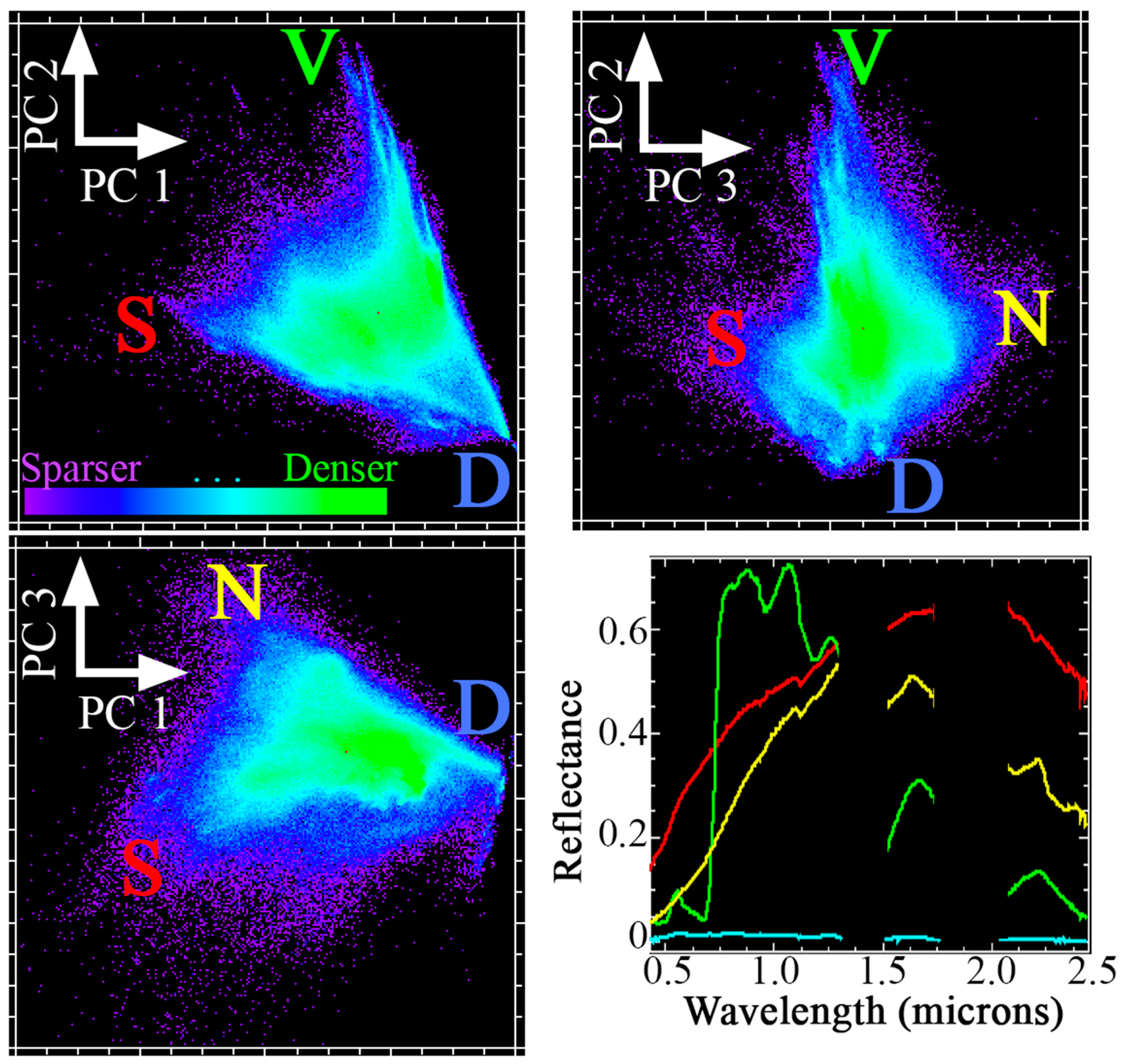
The low-order spectral feature space of the AVIRIS-ng reflectance mosaic is shown as orthogonal projections of the low order principal component (PC) distributions in Figure 2. The first three dimensions are found to capture >97% of the overall variance. The first two dimensions of the spectral feature space are bounded by spectral endmembers (EMs) corresponding to soil and rock Substrates, illuminated photosynthetic Vegetation, and Dark targets such as shadow, water, and low-albedo (S, V, and D). A clear non-photosynthetic vegetation (N) EM also emerges in the third dimension. Both the 3-EM (SVD) and 4-EM (SVDN) models were inverted and compared. V fraction (Fv) estimates from the the 3-EM and 4-EM models were found to be strongly interrelated (r > 0.99; MI = 1.9). Fv from the 3-EM model was used for subsequent analysis.
Bivariate distributions of VIs from SuperDove (y-axis) and Fv from mixture model inversion (x-axis) are shown in Figure 3. The DVI and NIRv were very strongly interrelated (DVI:NIRv ρ > 0.99; MI > 2.4; Figure S1). The DVI and NIRv were also colinear to Fv (ρ = 0.95 and MI = 1.4 for both DVI:Fv and NIRv:Fv), but substantially biased towards an underestimation at higher values (slope = 1.43, intercept = 0.017; regression in Figure S1). Similarly, the EVI and EVI2 were also strongly colinear (EVI:EVI2 ρ > 0.99; MI > 2.3; Figure S1). The EVI and EVI2 also correlated strongly with Fv (ρ > 0.94; MI > 1.2), showing some overestimation but considerably less bias than the DVI or NIRv.
In contrast, the NDVI and SR showed considerably more complex relationships with Fv. Both ρ (0.84 and 0.81) and MI (<0.7) were much lower than for other indices (Table S3). Consistent with previous comparisons to multispectral mixture models [27,38,39], the NDVI considerably overestimated Fv throughout most of its range, saturating near 0.6. Sensitivity to background reflectance was also especially apparent for the NDVI—for instance, spectra with Fv = 0.2 were found to exhibit NDVI values ranging from 0.05 to 0.6.
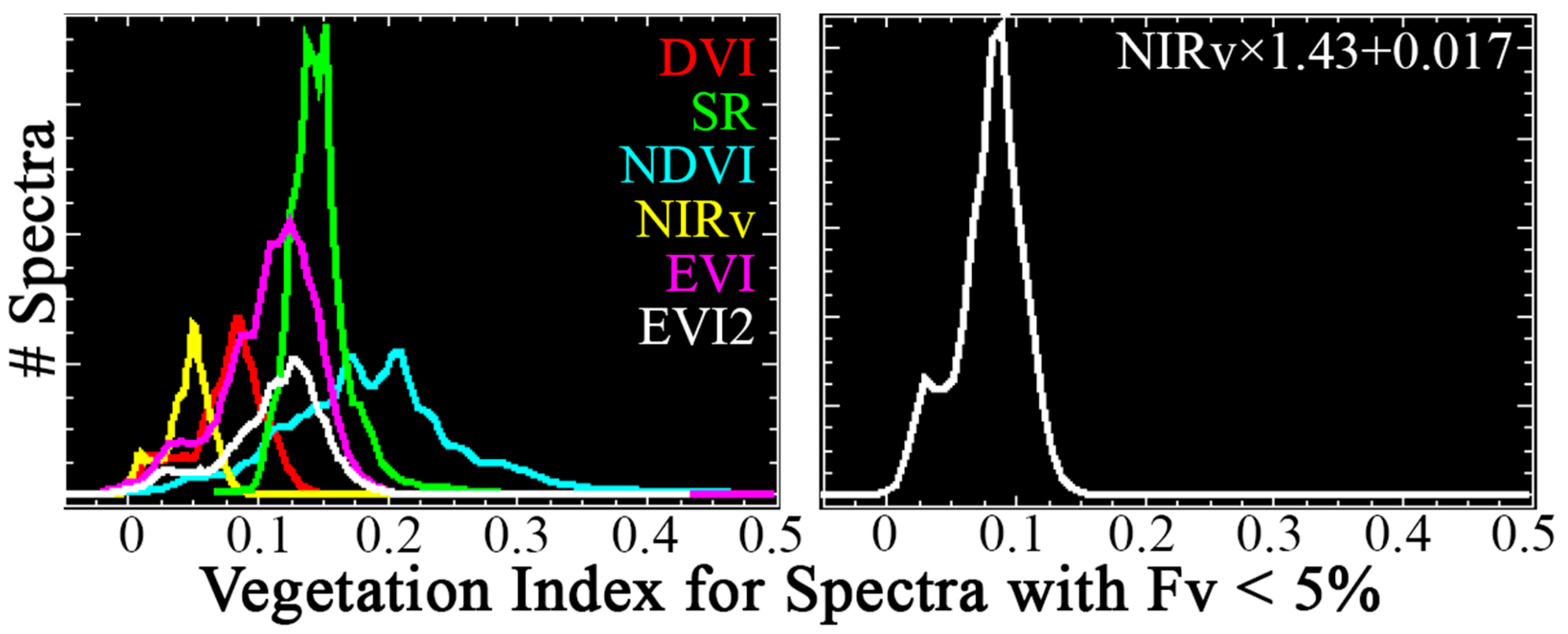
Univariate VI distributions for unvegetated (Fv < 0.05) spectra shown in Figure 4 quantify the sensitivity of each index to substrate and NPV background reflectance. Histograms show only spectra with Fv < 0.05 as estimated using the spectral mixture model. Of the indices, the NIRv (yellow) exhibited the least sensitivity to background reflectance, with a mode near 0.05 and standard deviation (s) = 0.018. The DVI (red) demonstrated slightly more sensitivity, with a greater mode (0.08) and dispersion (s = 0.029). The EVI (magenta) and EVI2 (white) performed similarly to each other, with greater modes (0.12) and dispersions (s = 0.038). Interestingly, the SR (green) performed similarly to the EVI and EVI2, with a similar mode (0.14) and lower dispersion (s = 0.018). Consistent with the bivariate distributions shown in Figure 3, the NDVI (cyan) demonstrated the most severe sensitivity to substrate background, with a modal value for unvegetated spectra above 0.2, higher dispersion (s = 0.083), and an upper tail extending beyond 0.5.
Both metrics of statistical similarity are found to yield similar overall patterns. Pairwise values (Tables S2 and S3 and Figure S1) are approximated via a monotonic, log-linear relationship. An important exception is found for the SR:NDVI relationship, which deviates markedly towards high MI values (MI > 10) without a coincident increase in ρ (further discussed below).

4. Discussion

4.1. Vegetation Index Intercomparison

A principal finding of this analysis is the observed high correlations of two pairs of vegetation indices: EVI with EVI2, and DVI with NIRv. The similarity between EVI and EVI2 confirms the potential for the EVI2 to serve as a representative proxy for EVI when a blue band is unavailable. The strong correlation and low bias between both these indices and Fv supports their use for the estimation of vegetation abundance in cases where SWIR bands are not available. Likewise, the similarity of DVI and NIRv, at least for this diverse agricultural mosaic, is striking (ρ > 0.99; MI = 2.45, 99% of |DVI-NIRv| < 0.07). The minimal sensitivity to background reflectance trades off with the overall underestimation of Fv. While this can be corrected using a simple linear bias correction, this correction increases sensitivity to background reflectance for sparse vegetation.
In contrast, NDVI and SR deviate from all four other VIs in important ways. NDVI in particular is challenged by saturation at mid-to-upper values and sensitivity to background reflectance at mid-to-lower values, both of which are clearly more severe than for the other VIs. These findings extend previous results based on datasets collected at coarser spatial and spectral resolution [27,38,39,40,41] to 3 m imaging spectroscopy, and agree with a large amount of the literature (e.g., [42,43], including a recent multiscale results correlating to cover crop biomass [24]). Concordance with these studies suggests it is reasonable to expect the results of this analysis—including the striking heteroskedasticity, nonlinearity, and background reflectance sensitivity of NDVI and SR—to generalize to other current and future satellite (and airborne) multispectral sensors such as those on the WorldView, Pleiades, Landsat, and Sentinel-2 platforms. Further, because this analysis simulates SuperDove data directly from AVIRIS-ng, the entirety of the observed relationship between VIs and mixture fractions can be attributed to the spectral modeling step alone (rather than acquisition-specific idiosyncrasies such as view and illumination angle).

4.2. Similarity Metrics

Another finding of this analysis is the correspondence between parametric (Pearson correlation coefficient, ρ) and nonparametric (mutual information, MI) methods of quantifying statistical similarity and information content. This consistency strengthens the findings of the VI intercomparison, as both methods show strong relationships between [Fv] and [DVI, NIRv, EVI, and EVI2] but much weaker relationships between [Fv] and [SR, NDVI]. Reduced MI values for the NDVI suggest that the limitations of the index are yet more pernicious than simply being due to a nonlinear, heteroskedastic relationship (which should be better captured via MI). This is supported by the broader dispersion of the NDVI distribution than is evident in DVI, NIRv, EVI, or EVI2, as seen in Figure 3. Note also that NDVI and SR have, by far, the largest value of MI (11.33) of any pair of indices, consistent with their demonstrable nonlinear relationship (Figure S1, lower right). This is due to a functional dependence between the two indices, further explored in Figure S1 and Analytical Exercise S1. Such behavior is notably absent for the NDVI:Fv and SR:Fv relationships, which do not markedly deviate above ρ:MI loglinearity, suggesting that even nonlinear regression is unlikely to be effective in capturing this variability.

4.3. Dimensionality and Spectral Endmembers

Another important finding of this analysis is the broad agreement with previous studies in terms of both spectral dimensionality [31,44,45,46,47] and the generality of S,V,D endmember spectra and associated mixture model [27,31,38,46,48]. The prominence of the NPV EM is more evident than in some prior studies, which may be due to the focus of the study on late summer agricultural landscapes with spatially extensive monocultures of dense vegetation at various stages in its life cycle. In this study, the clear differentiation of S and N EMs along PC3 is especially interesting given the dichotomy of (1) the broad similarity of their spectral continua versus (2) the important differences in cellulose/lignin absorption features at SWIR wavelengths [49].

4.4. Limitations and Future Work

This study was designed to compare the theoretical performance of various multispectral vegetation indices against the results from a hyperspectral mixture model. Deriving simulated Planet SuperDove reflectance directly from atmospherically corrected AVIRIS-ng spectra controls for differences in sun-sensor geometry, sensor-to-sensor radiometric miscalibration, image coregistration, and atmospheric correction that would bias a comparison of independently collected observations. We note that radiometric and BRDF differences may be especially significant for Planet data, given the known limitations of the Dove/SuperDove fleet and the constantly evolving remedies [8,50,51]. Additionally, by convolving AVIRIS-ng reflectance spectra to SuperDove spectral response functions after applying ISOFIT, it is likely that the simulated SuperDove spectra exhibit substantially more accurate atmospheric correction than would be possible using SuperDove radiance spectra directly. This is most likely to impact results for EVI, given its use of the visible blue band. Moving forward, a comparative analysis of EVI and EVI2 computed from a comparably diverse compilation of SuperDove-observed reflectance spectra might provide a constraint on the effectiveness of atmospheric correction and could be an interesting avenue for future work.

5. Conclusions

This study addressed the fundamental question of linking multispectral vegetation indices to hyperspectral mixture models for agricultural applications. Using a compilation of 125 subsets from 15 airborne imaging spectroscopy flight lines spanning a diverse agricultural mosaic, we simulated 64,000,000 multispectral SuperDove reflectance spectra and used them to compute 6 commonly used vegetation indices. We then compared these indices against the photosynthetic vegetation fraction estimated from the inversion of a linear mixture model applied to the original 5 nm hyperspectral data (Fv). We quantified complementary aspects of the bivariate distributions using both parametric (ρ) and nonparametric (MI) metrics. DVI and NIRv were strongly colinear (ρ > 0.99; MI = 2.45) and approximately linearly related to Fv (ρ > 0.95; MI > 1.4), with minimal sensitivity to the substrate background reflectance (0 to 0.1 for unvegetated spectra) but substantial deviation from 1:1 (the DVI and NIRv values of 0.6 for Fv values of 1.0). EVI and EVI2 also performed similarly to each other (ρ > 0.99; MI = 2.3) and were also approximately linear to Fv (ρ = 0.95; MI > 1.2), but with both a more prominent impact of background reflectance (0 to 0.2 for unvegetated spectra) and greatly reduced deviation from 1:1. Of the indices, NDVI and SR exhibited by far the weakest relationships to Fv (ρ = 0.84 and 0.81; MI = 0.69). NDVI in particular showed severe saturation effects and sensitivity to soil background reflectance. Comparison of parametric (ρ) and nonparametric (MI) similarity statistics yielded a roughly log-linear relationship, with a notable exception supporting a nonlinear analytical relationship between NDVI and SR. Notably, because SuperDove data were simulated directly from AVIRIS-ng, results can be attributed to the spectral modeling step alone (and thus isolated from acquisition-specific idiosyncrasies such as the view and illumination angle).
Taken together, this analysis suggests that for agricultural applications:
  • EVI2 can likely serve as a proxy for EVI in situations where a blue band is not available, and both can serve as proxies for Fv in situations where SWIR bands are not available.
  • DVI and NIRv yield very similar values (ρ > 0.99, 99% of |DVI-NIRv| < 0.07).
  • DVI and NIRv show low sensitivity to substrate background reflectance, but systematically underestimate Fv. A linear bias correction reduces deviation from 1:1 but increases substrate background effects.
  • Bivariate distributions of ρ and the MI can usefully contextualize nonlinear VI relationships.
  • As metrics of subpixel vegetation abundance, NDVI and SR exhibit severe challenges in nonlinearity, heteroskedasticity, and sensitivity to substrate background reflectance.

Supplementary Materials

The following supporting information can be downloaded at: https://www.mdpi.com/article/10.3390/rs15040971/s1, Figure S1: additional VI relationships; Figure S2: parametric versus nonparametric statistics; Table S1: AVIRIS-ng flightlines used for this analysis; Table S2: mutual information matrix; Table S3: correlation matrix; analytical exercise S1: An exploration of the relationship between the SR and NDVI.

Author Contributions

Conceptualization, D.S. and C.S.; methodology, D.S. and C.S.; formal analysis, D.S. and C.S.; investigation, D.S. and C.S.; resources, D.S. and C.S.; data curation, D.S. and C.S.; writing—original draft preparation, D.S.; writing—review and editing, D.S. and C.S.; visualization, D.S. and C.S.; funding acquisition, D.S. and C.S. All authors have read and agreed to the published version of the manuscript.

Funding

D.S. was supported by the USDA NIFA Sustainable Agroecosystems Program under Grant # 2022-67019-36397; the NASA Land-Cover/Land-Use Change Program under Grant # NNH21ZDA001N-LCLUC; the NASA Remote Sensing of Water Quality Program under Grant # 80NSSC22K0907; and the NSF Signals in the Soil Program under Award # 2226649. C.S. was supported by the endowment of the Lamont Doherty Earth Observatory of Columbia University.

Data Availability Statement

The data supporting this manuscript can be downloaded free of charge from the web portal listed in the main text.

Acknowledgments

The authors thank the National Center for Ecological Analysis and Synthesis (NCEAS) for providing computational resources that supported this work, and three anonymous reviewers for constructive feedback.

Conflicts of Interest

The authors declare no conflict of interest.

References

  1. Thompson, D.R.; Schimel, D.S.; Poulter, B.; Brosnan, I.; Hook, S.J.; Green, R.O.; Glenn, N.; Guild, L.; Henn, C.; Cawse-Nicholson, K. NASA’s Surface Biology and Geology Concept Study: Status and Next Steps; IEEE: New York, NY, USA, 2021; pp. 3269–3271. [Google Scholar]
  2. Candela, L.; Formaro, R.; Guarini, R.; Loizzo, R.; Longo, F.; Varacalli, G. The PRISMA Mission. In Proceedings of the 2016 IEEE International Geoscience and Remote Sensing Symposium (IGARSS), Beijing, China, 10 July 2016; pp. 253–256. [Google Scholar]
  3. Iwasaki, A.; Ohgi, N.; Tanii, J.; Kawashima, T.; Inada, H. Hyperspectral Imager Suite (HISUI)-Japanese Hyper-Multi Spectral Radiometer; IEEE: New York, NY, USA, 2011; pp. 1025–1028. [Google Scholar]
  4. Guanter, L.; Kaufmann, H.; Segl, K.; Foerster, S.; Rogass, C.; Chabrillat, S.; Kuester, T.; Hollstein, A.; Rossner, G.; Chlebek, C. The EnMAP Spaceborne Imaging Spectroscopy Mission for Earth Observation. Remote Sens. 2015, 7, 8830–8857. [Google Scholar] [CrossRef]
  5. Green, R.O.; Mahowald, N.; Ung, C.; Thompson, D.R.; Bator, L.; Bennet, M.; Bernas, M.; Blackway, N.; Bradley, C.; Cha, J.; et al. The Earth Surface Mineral Dust Source Investigation: An Earth Science Imaging Spectroscopy Mission. In Proceedings of the 2020 IEEE Aerospace Conference, Big Sky, MT, USA, 7 March 2020; pp. 1–15. [Google Scholar]
  6. Liu, H.; Bruning, B.; Garnett, T.; Berger, B. Hyperspectral Imaging and 3D Technologies for Plant Phenotyping: From Satellite to Close-Range Sensing. Comput. Electron. Agric. 2020, 175, 105621. [Google Scholar] [CrossRef]
  7. Safyan, M. Planet’s Dove Satellite Constellation. In Handbook of Small Satellites: Technology, Design, Manufacture, Applications, Economics and Regulation; Springer: Berlin/Heidelberg, Germany, 2020; pp. 1–17. [Google Scholar]
  8. Leach, N.; Coops, N.C.; Obrknezev, N. Normalization Method for Multi-Sensor High Spatial and Temporal Resolution Satellite Imagery with Radiometric Inconsistencies. Comput. Electron. Agric. 2019, 164, 104893. [Google Scholar] [CrossRef]
  9. Kriegler, F.; Malila, W.; Nalepka, R.; Richardson, W. Preprocessing Transformations and Their Effects on Multispectral Recognition. Remote Sens. Environ. 1969, VI, 97. [Google Scholar]
  10. Tucker, C.J. Red and Photographic Infrared Linear Combinations for Monitoring Vegetation. Remote Sens. Environ. 1979, 8, 127–150. [Google Scholar] [CrossRef]
  11. Rouse, J.; Haas, R.H.; Deering, D.; Schell, J.; Harlan, J.C. Monitoring the Vernal Advancement and Retrogradation (Green Wave Effect) of Natural Vegetation. U.S. Patent 19730017588, 1 April 1974. [Google Scholar]
  12. Huete, A. A Soil-Adjusted Vegetation Index (SAVI). Remote Sens. Environ. 1988, 25, 295–309. [Google Scholar] [CrossRef]
  13. Huete, A.; Didan, K.; Miura, T.; Rodriguez, E.P.; Gao, X.; Ferreira, L.G. Overview of the Radiometric and Biophysical Performance of the MODIS Vegetation Indices. Remote Sens. Environ. 2002, 83, 195–213. [Google Scholar] [CrossRef]
  14. Jiang, Z.; Huete, A.; Didan, K.; Miura, T. Development of a Two-Band Enhanced Vegetation Index without a Blue Band. Remote Sens. Environ. 2008, 112, 3833–3845. [Google Scholar] [CrossRef]
  15. Badgley, G.; Field, C.B.; Berry, J.A. Canopy Near-Infrared Reflectance and Terrestrial Photosynthesis. Sci. Adv. 2017, 3, e1602244. [Google Scholar] [CrossRef]
  16. Wulder, M.A.; Masek, J.G.; Cohen, W.B.; Loveland, T.R.; Woodcock, C.E. Opening the Archive: How Free Data Has Enabled the Science and Monitoring Promise of Landsat. Remote Sens. Environ. 2012, 122, 2–10. [Google Scholar] [CrossRef]
  17. Claverie, M.; Ju, J.; Masek, J.G.; Dungan, J.L.; Vermote, E.F.; Roger, J.-C.; Skakun, S.V.; Justice, C. The Harmonized Landsat and Sentinel-2 Surface Reflectance Data Set. Remote Sens. Environ. 2018, 219, 145–161. [Google Scholar] [CrossRef]
  18. Neigh, C.S.; Masek, J.G.; Nickeson, J.E. High-resolution Satellite Data Open for Government Research. Eos Trans. Am. Geophys. Union 2013, 94, 121–123. [Google Scholar] [CrossRef]
  19. Zhang, C.; Marzougui, A.; Sankaran, S. High-Resolution Satellite Imagery Applications in Crop Phenotyping: An Overview. Comput. Electron. Agric. 2020, 175, 105584. [Google Scholar] [CrossRef]
  20. Du, J.; Kimball, J.S.; Bindlish, R.; Walker, J.P.; Watts, J.D. Local Scale (3-m) Soil Moisture Mapping Using SMAP and Planet SuperDove. Remote Sens. 2022, 14, 3812. [Google Scholar] [CrossRef]
  21. Johansen, K.; Ziliani, M.G.; Houborg, R.; Franz, T.E.; McCabe, M.F. CubeSat Constellations Provide Enhanced Crop Phenology and Digital Agricultural Insights Using Daily Leaf Area Index Retrievals. Sci. Rep. 2022, 12, 5244. [Google Scholar] [CrossRef]
  22. Alemu, W.G.; Neigh, C.S.R. Desert Locust Cropland Damage Differentiated from Drought, with Multi-Source Remote Sensing in Ethiopia. Remote Sens. 2022, 14, 1723. [Google Scholar] [CrossRef]
  23. Zhou, X.; Li, Y.; Sun, Y.; Su, Y.; Li, Y.; Yi, Y.; Liu, Y. Research on Dynamic Monitoring of Grain Filling Process of Winter Wheat from Time-Series Planet Imageries. Agronomy 2022, 12, 2451. [Google Scholar] [CrossRef]
  24. Swoish, M.; Da Cunha Leme Filho, J.F.; Reiter, M.S.; Campbell, J.B.; Thomason, W.E. Comparing Satellites and Vegetation Indices for Cover Crop Biomass Estimation. Comput. Electron. Agric. 2022, 196, 106900. [Google Scholar] [CrossRef]
  25. Xue, J.; Su, B. Significant Remote Sensing Vegetation Indices: A Review of Developments and Applications. J. Sens. 2017, 2017, 1353691. [Google Scholar] [CrossRef]
  26. Zeng, Y.; Hao, D.; Huete, A.; Dechant, B.; Berry, J.; Chen, J.M.; Joiner, J.; Frankenberg, C.; Bond-Lamberty, B.; Ryu, Y.; et al. Optical Vegetation Indices for Monitoring Terrestrial Ecosystems Globally. Nat. Rev. Earth Environ. 2022, 3, 477–493. [Google Scholar] [CrossRef]
  27. Small, C.; Milesi, C. Multi-Scale Standardized Spectral Mixture Models. Remote Sens. Environ. 2013, 136, 442–454. [Google Scholar] [CrossRef] [Green Version]
  28. Chapman, J.W.; Thompson, D.R.; Helmlinger, M.C.; Bue, B.D.; Green, R.O.; Eastwood, M.L.; Geier, S.; Olson-Duvall, W.; Lundeen, S.R. Spectral and Radiometric Calibration of the Next Generation Airborne Visible Infrared Spectrometer (AVIRIS-NG). Remote Sens. 2019, 11, 2129. [Google Scholar] [CrossRef]
  29. Thompson, D.R.; Natraj, V.; Green, R.O.; Helmlinger, M.C.; Gao, B.-C.; Eastwood, M.L. Optimal Estimation for Imaging Spectrometer Atmospheric Correction. Remote Sens. Environ. 2018, 216, 355–373. [Google Scholar] [CrossRef]
  30. CDFA. California Agricultural Statistics Review, 2020–2021; California Department of Food and Agriculture: Sacramento, CA, USA, 2021; p. 156. [Google Scholar]
  31. Sousa, D.; Small, C. Multisensor Analysis of Spectral Dimensionality and Soil Diversity in the Great Central Valley of California. Sensors 2018, 18, 583. [Google Scholar] [CrossRef]
  32. Richardson, A.J.; Wiegand, C. Distinguishing Vegetation from Soil Background Information. Photogramm. Eng. Remote Sens. 1977, 43, 1541–1552. [Google Scholar]
  33. Shannon, C.E. A Mathematical Theory of Communication. Bell Syst. Tech. J. 1948, 27, 379–423. [Google Scholar] [CrossRef]
  34. Kozachenko, L.F.; Leonenko, N.N. Sample Estimate of the Entropy of a Random Vector. Probl. Peredachi Inf. 1987, 23, 9–16. [Google Scholar]
  35. Ross, B.C. Mutual Information between Discrete and Continuous Data Sets. PloS One 2014, 9, e87357. [Google Scholar] [CrossRef] [PubMed]
  36. Kraskov, A.; Stögbauer, H.; Grassberger, P. Estimating Mutual Information. Phys. Rev. E 2004, 69, 066138. [Google Scholar] [CrossRef] [PubMed]
  37. NRCS Soil Survey Staff, Natural Resources Conservation Service, United States Department of Agriculture. Web Soil Survey. 2022. Available online: https://websoilsurvey.sc.egov.usda.gov/App/WebSoilSurvey.aspx (accessed on 1 June 2022).
  38. Sousa, D.; Small, C. Global Cross-Calibration of Landsat Spectral Mixture Models. Remote Sens. Environ. 2017, 192, 139–149. [Google Scholar] [CrossRef]
  39. Sousa, D.; Small, C. Globally Standardized MODIS Spectral Mixture Models. Remote Sens. Lett. 2019, 10, 1018–1027. [Google Scholar] [CrossRef]
  40. Elmore, A.J.; Mustard, J.F.; Manning, S.J.; Lobell, D.B. Quantifying Vegetation Change in Semiarid Environments: Precision and Accuracy of Spectral Mixture Analysis and the Normalized Difference Vegetation Index. Remote Sens. Environ. 2000, 73, 87–102. [Google Scholar] [CrossRef]
  41. Small, C. Estimation of Urban Vegetation Abundance by Spectral Mixture Analysis. Int. J. Remote Sens. 2001, 22, 1305–1334. [Google Scholar] [CrossRef]
  42. Gitelson, A.A. Wide Dynamic Range Vegetation Index for Remote Quantification of Biophysical Characteristics of Vegetation. J. Plant Physiol. 2004, 161, 165–173. [Google Scholar] [CrossRef]
  43. Myneni, R.B.; Hall, F.G.; Sellers, P.J.; Marshak, A.L. Marshak The Interpretation of Spectral Vegetation Indexes. IEEE Trans. Remote Sens. 1995, 33, 481–486. [Google Scholar] [CrossRef]
  44. Boardman, J.W.; Green, R.O. Exploring the Spectral Variability of the Earth as Measured by AVIRIS in 1999. In Proceedings of the Summaries of the 8th Annu. JPL Airborne Geosci. Workshop; NASA: Pasadena, CA, USA, 2000; Volume 1, pp. 1–12. [Google Scholar]
  45. Thompson, D.R.; Boardman, J.W.; Eastwood, M.L.; Green, R.O. A Large Airborne Survey of Earth’s Visible-Infrared Spectral Dimensionality. Opt. Express 2017, 25, 9186–9195. [Google Scholar] [CrossRef] [PubMed]
  46. Sousa, D.; Brodrick, P.G.; Cawse-Nicholson, K.; Fisher, J.B.; Pavlick, R.; Small, C.; Thompson, D.R. The Spectral Mixture Residual: A Source of Low-Variance Information to Enhance the Explainability and Accuracy of Surface Biology and Geology Retrievals. J. Geophys. Res. Biogeosciences 2022, 127, e2021JG006672. [Google Scholar] [CrossRef]
  47. Cawse-Nicholson, K.; Hook, S.J.; Miller, C.E.; Thompson, D.R. Intrinsic Dimensionality in Combined Visible to Thermal Infrared Imagery. IEEE J. Sel. Top. Appl. Earth Obs. Remote Sens. 2019, 12, 4977–4984. [Google Scholar] [CrossRef]
  48. Small, C. The Landsat ETM+ Spectral Mixing Space. Remote Sens. Environ. 2004, 93, 1–17. [Google Scholar] [CrossRef]
  49. Roberts, D.A.; Smith, M.O.; Adams, J.B. Green Vegetation, Nonphotosynthetic Vegetation, and Soils in AVIRIS Data. Remote Sens. Environ. 1993, 44, 255–269. [Google Scholar] [CrossRef]
  50. Wegmueller, S.A.; Leach, N.R.; Townsend, P.A. LOESS Radiometric Correction for Contiguous Scenes (LORACCS): Improving the Consistency of Radiometry in High-Resolution Satellite Image Mosaics. Int. J. Appl. Earth Obs. Geoinf. 2021, 97, 102290. [Google Scholar] [CrossRef]
  51. Vanhellemont, Q. Daily Metre-Scale Mapping of Water Turbidity Using CubeSat Imagery. Opt. Express 2019, 27, A1372–A1399. [Google Scholar] [CrossRef] [PubMed]
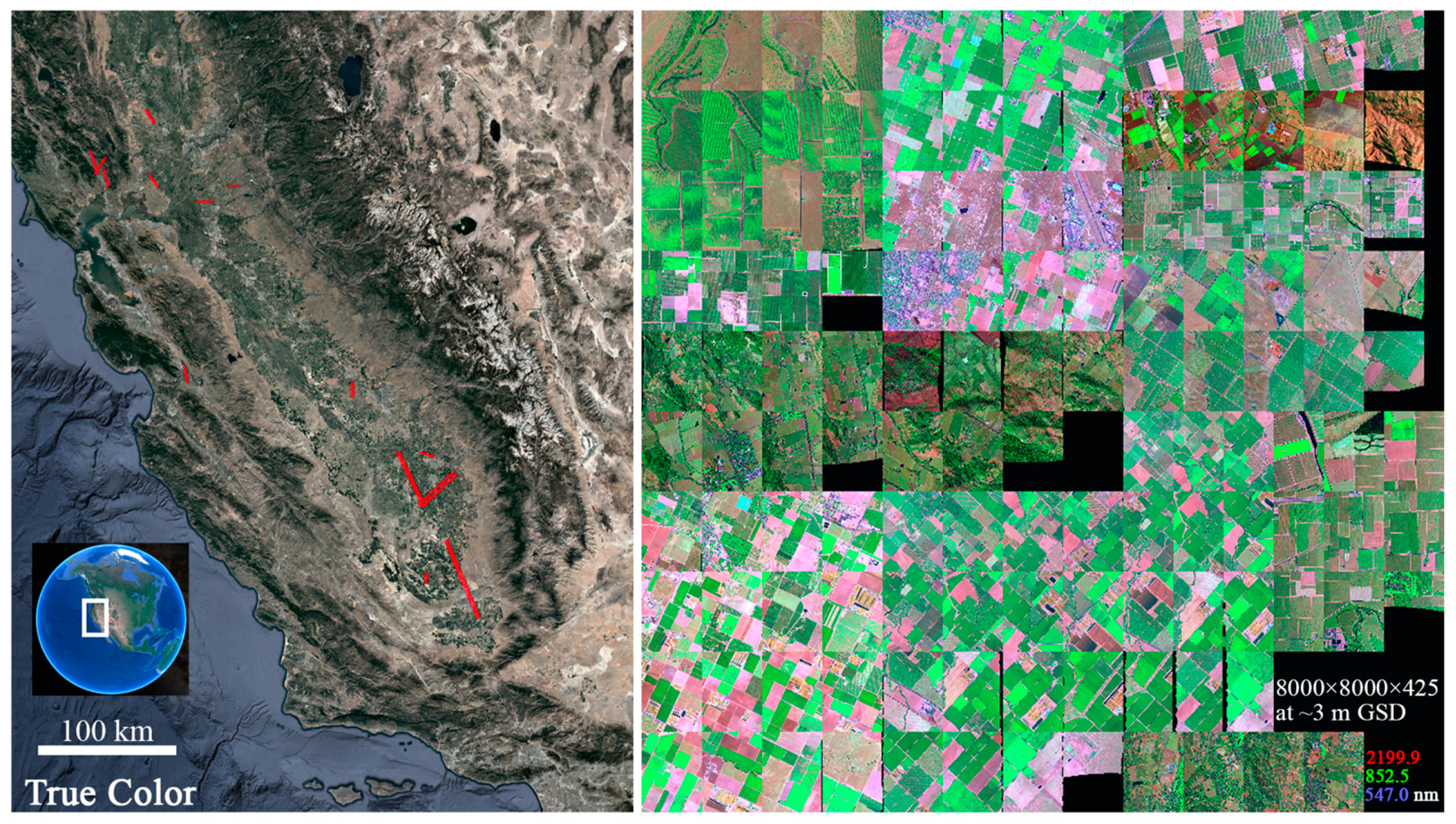
Figure 1. Index map. (Left): 15 flight lines from the 2020 AVIRIS-ng campaign (red) span broad crop and soil diversity in one of the most productive agricultural regions on earth. (Right): false color composite mosaic image compiled from 125 subsets, each of 600 × 800 pixels (~2.4 × 3.2 km). Ground sampling distance for all lines is approximately 3 m. For further information about soil diversity, see [31,37]; for agricultural diversity see [30].
Remotesensing 15 00971 g001
Figure 2. Spectral feature space and endmembers. The first 3 dimensions of the spectral feature space, visualized here, account for over 97% of the variance in the AVIRIS-ng spectra. Substrate, vegetation and dark (S, V, D) endmembers bound the first two dimensions of this feature space. Non- photosynthetic vegetation (N) extends the plane of substrates in the third dimension. Compare to previous results from mosaics of AVIRIS-classic and Landsat [31]. Colors represent point density, from sparser (violet) to denser (green).
Remotesensing 15 00971 g002
Figure 3. Bivariate distributions of spectral indices versus vegetation fraction. Six commonly used multispectral indices (y-axis) are compared to photosynthetic vegetation fraction (Fv) computed directly from hyperspectral AVIRIS-ng reflectances (x-axis). DVI and NIRv are highly correlated with each other (0.99) and with Fv (0.95), but not near the 1:1 line (red). Similarly, EVI and EVI2 are also highly correlated with each other (0.99) and with Fv (0.94 or 0.95). NDVI and SR exhibit substantially reduced correlation to Fv (0.84 and 0.81). Mutual information (MI) generally agrees with these correlations. MI values (relative to Fv) for DVI, NIRv, EVI, and EVI2 are all 1.35 +/− 0.1. NDVI and SR MI values are lower, each at 0.69. SR* indicates that values are scaled by 0.1 for visualization. Spectra with values < −0.2 or >1.2 are excluded. All Pearson correlation values are significantly different from the uncorrelated null hypothesis (p < 0.01). Bootstrapping via random selection of 30% of data values resulted in MI variability on the order of 0.01 or less.
Remotesensing 15 00971 g003
Figure 4. Spectral index distributions for unvegetated spectra. (Left): histograms show VI values for all spectra with <5% photosynthetic vegetation cover, as estimated from inversion of the AVIRIS-ng spectral mixture model. NIRv values are closest to zero with nearly all values < 0.1 and a mode near 0.05. DVI is characterized by a mode near 0.08 and greater dispersion. EVI and EVI2 both show modes near 0.12. SR modal value is near EVI, but with less dispersion. NDVI shows, by far, the highest mode (>0.2) and largest dispersion (NDVI for some unvegetated spectra as large as 0.5). (Right): histogram of NIRv values after linear regression is applied. For the distribution of regressed NIRv, mean = 0.08 and standard deviation = 0.026.
Remotesensing 15 00971 g004
Table 1. Spectral index formulas. All indices computed from simulated SuperDove spectra.
Index NameAcronymFormula
Difference vegetation (veg.) indexDVINIR − Red
Normalized difference veg. indexNDVI(NIR − Red)/(NIR + Red)
Near-infrared reflectance of veg.NIRvNIR × (NIR − Red)/(NIR + Red)
Simple ratioSRNIR/Red
Enhanced veg. indexEVI2.5 × (NIR − Red)/(NIR + 6 × Red − 7.5 × Blue + 1)
2-band Enhanced veg. indexEVI22.5 × (NIR − Red)/(NIR + 2.4 × Red + 1)
Disclaimer/Publisher’s Note: The statements, opinions and data contained in all publications are solely those of the individual author(s) and contributor(s) and not of MDPI and/or the editor(s). MDPI and/or the editor(s) disclaim responsibility for any injury to people or property resulting from any ideas, methods, instructions or products referred to in the content.