A New Strategy to Fuse Remote Sensing Data and Geochemical Data with Different Machine Learning Methods

Abstract

Geochemical data can reflect geological features, making it one of the basic types of geodata that have been widely used in mineral exploration, environmental assessment, resource potential analysis and other research. However, final decisions regarding activities are often limited by the spatial accuracy of geochemical data. Geochemical sampling is sometimes difficult to conduct because of harsh natural and geographic conditions (e.g., mountainous areas with high altitude and complex terrain), meaning that only medium/low-precision survey data could be obtained, which may not be adequate for regional geochemical mapping and exploration. Modern techniques such as remote sensing could be used to address this issue. In recent decades, the development of remote sensing technology has provided a huge amount of earth observation data with high spatial, temporal and spectral resolutions. The advantage of rapid acquisition of spatial and spectral information of large areas has promoted the broad use of remote sensing data in geoscientific research. Remote sensing data can help to differentiate various ground features by recording the electromagnetic response of the surface to solar radiation. Many problems that occur during the process of fusing remote sensing and geochemical data have been reported, such as the feasibility of existing fusion methods and low fusion accuracies that are less useful in practice. In this paper, a new strategy for integrating geochemical data and remote sensing data (referred to as ASTER data) is proposed; this strategy is achieved through linear regression as well as random forest and support vector regression algorithms. The results show that support vector regression can obtain better results for the available data sets and prove that the strategy currently proposed can effectively support the fusion of high-spatial-resolution remote sensing data (15 m) and low-spatial-resolution geochemical data (2000 m) in wide-range accurate geochemical applications (e.g., lithological identification and geochemical exploration).

1. Introduction

As an important geological data set, geochemical data plays an important role in ecological environment survey [1,2], geological mapping, mineral exploration [3], industrial decision-making, land suitability evaluation and other fields. Geochemical data can reveal the impacts of human activities on ecology and environment. Several studies have pointed out that some agricultural, mining and industrial activities will lead to the release of harmful elements to the environment, potentially causing adverse effects to ecosystems and human health [4,5]. In the field of geology, geochemical data can be analyzed with statistical theories to help determine the existence of geologic units and delineate mineral exploitation targets [6]. Moreover, in recent years, there have been considerable developments in the broad application of deep learning, machine learning and artificial intelligence methods to integrate geochemical data with other multi-source geoscience data to reach this goal [7,8].

Unlike the time-consuming and laborious process of geochemical sampling, remote sensing techniques can acquire spectral information about ground features quickly and efficiently. The spectral information recorded by the remote sensing data is determined by the interactive characteristics between electromagnetic waves and ground objects, that is, the spectral characteristics of ground objects [9]. Previous studies have shown that diagnostic absorption features (e.g., the wavelength and depth of absorption) of ground objects are closely related to the molecular vibration forms and electron transition behaviors of the different molecules [10]. In recent years, some studies have revealed that the responses of ground objects to electromagnetic waves displayed in remote sensing data are also correlated with the content of geochemical elements. For example, the difference in the aluminum content present in the white micas that are widely distributed in the intermediate-felsic magmatic rocks can be presented by the wavelength of diagnostic absorption peak of these minerals. The shorter the wavelength corresponding to the characteristic absorption peak, the higher the content of aluminum in white micas [11]. This finding makes it possible to determine mineral composition and classify rocks with remote sensing data, as the types and content of white micas in different lithologies follow certain rules. For example, Kokaly et al. [12] used HyMap imaging spectrometer data for the area of Orange Hill–Bond Creek, Alaska, and illustrated longer wavelengths of white mica’s diagnostic absorption feature that occurs at approximately 2200 nm; these wavelengths were associated with a porphyry cluster and enrichment of Cu. A longward shift of the diagnostic absorption peak in the continuum removed the white mica 2200 nm combination feature in hyperspectral data that was collected at the Cripple Creek & Victor Mine in Cripple Creek, CO, USA, demonstrating a decrease of Al and an increase in the depth of the open pit [13]. Swayze et al. [14] successfully developed acidic mineral distribution maps using AVIRIS data. In addition, the spatial distribution pattern of nutrient content or heavy metal elements contained in soil and water can be derived using spectroscopy based on the intrinsic relationship between the geochemical and remotely sensed data [15]. Using reflectance spectra data to solve geochemical problems has become a common practice in recent years as the application effects have been proven to be significant.

From the aspect of geology, geochemical data can provide indicative information for mineral exploration. However, due to the broad span of sampling media and the extensive presence of various elements in different geologic bodies, the indication of geochemical anomalies that represent geologic bodies is often obscure. With abundant spectral information, remote sensing data can distinguish ground objects with physical characteristics due to the differences in the reflection spectrum of various ground objects. Combining remote sensing and geochemical data can effectively make full use of the advantages of the two data sets in the identification of ground objects. The use of fusion algorithms to comprehensively analyze geochemical and remote sensing data has a long history. Early remote sensing and geochemical data image fusion algorithms focused on linear methods; for example, IHS transformation has been used to fuse Landsat MSS and geochemical data to find gold anomalies and alteration zones [16]. Geological, geochemical, and remote sensing data are also used in Iran for principal component analysis; this function can identify two mineralization types, including podiform chromite and epithermal gold-antimony mineralization types [17]. With the improvement of remote sensing data quality and the development of computer science, nonlinear methods in the field of image fusion have been gradually developed. Particularly, by introducing machine learning methods into geo-information integration, computer technology can help to obtain high-quality and efficient data fusion. Nowadays, machine learning algorithms (such as random forests, support vector machines, etc.) have been widely applied in the field of geology. Significant progress has been made in target recognition, such as geological disaster analysis and detection [18], mineral exploration [19], geochemical anomaly identification [20], etc. Machine learning methods based on lithologic mapping techniques have been significantly developed and improved, and remote sensing data is used to reveal the composition of materials and/or the relationship between geochemical components and their contents [21,22]. The intrinsic basis of these studies is to fuse remote sensing data with geochemical data to analyze the physicochemical properties of lithologic units. The commonly used remote sensing and geochemical data fusion methods include random forests, independent principal components, etc. [22,23,24]. However, due to the prominent differences in the spatial scales of remote sensing and geochemical data, the current fusion methods struggle to reflect the detailed information contained in remote sensing data [25], which may cause failures in generating ideal fusion results that are feasible or ready-to-use for real work. In addition, traditional geochemical interpolation methods, such as Inverse Distance Weighting (IDW) and Kriging, present their own inconveniences in practice. IDW is not effective for clustered samples, and the statistical conditions used for Kriging method are stricter. These may make the interpolation results of these two algorithms unsatisfactory for further analysis [26]. This contribution proposes a fusion strategy of remote sensing data and geochemical data, which supplements spatial details contained by the former to the latter, allowing the limitations of using traditional interpolation methods on the data to be fundamentally solved. Therefore, when remote sensing data is added, the generation of high-resolution geochemical data is no longer “self-simulation” but is instead “evidence based”. From the perspective of economy and convenience, both remote sensing data with rich spatial information and geochemical data at a smaller scale are relatively easy to acquire. The integration of remote sensing data and geochemical data based on the strategy proposed in the current research can reduce the difficulty of mineral exploration, resource and environmental survey and other related geological work without increasing the cost.

The Dacaotan area of the eastern Tianshan mineralization belt in Xinjiang, China is selected as this study’s research area of this study and where the fusion experiment of geochemical and remote sensing data will be conducted. The eastern Tianshan area is well known for its prominent polymetallic mineralization, such as copper, nickel, gold, etc. [27]. At the same time, this area is sparsely vegetated, and the extensive exposure of strata can maximize the advantages of remote sensing techniques in geological work. Through this study, high-precision geochemical data fused with remote sensing images can be obtained, which may provide new information for mineral exploration in the study area.

2. Material and Methodologies

2.1. Geological Background

Research was conducted in the eastern Tianshan Orogen area (Figure 1, red box) at coordinates from 91°9′32″E to 92°59′10″E and 41°52′53″N to 42°14′28″N. As part of the Central Asia Orogenic Belt, the eastern Tianshan Orogen is located in the junction zone of the Siberian, the Juggar-Kazakhstan and the Tarim blocks. The tectonic evolution of this orogenic belt is complex; each block has experienced collage formation, accretion–subduction and collisional orogeny of each block during the formation–extinction process of the Paleo-Asian ocean interplate [28,29,30,31]. The complex tectonic movement in the eastern Tianshan region not only formed the Paleozoic arc-basin systems [32,33,34], but also promoted the polymetallic mineralization which defined this area as an important metal mineral base in China [35].

Controlled by the main faults, the strata and magmatic rocks in eastern Tianshan are nearly E–W distributed and trending. The Dananhu-Tousuquan (or Dananhu-Harlik) arc in the north and the Aqishan-Yamansu arc in the south are separated by the Kanggur ductile shear zone [36]. The study area in this paper is located in the middle of the eastern Tianshan mineral district (Figure 1). Along the Dacaotan fault, the Dananhu-Tousuquan arc belt can be further divided into the Kalatag subzone in the north and the Xiaorequanzi-Tuwu subzone in the south [34]. The Kalatag subzone is characterized by a sequence of volcanic rocks made of intermediate-mafic volcanic rocks (e.g., basalt and andesite) in the Middle-Upper Ordovician Daliugou Formation, volcanic-sedimentary rocks (e.g., dacitic tuff) in the Lower Silurian Hongliuxia Formation, felsic volcanic rocks (mainly dacite) and pyroclastic rocks in the Lower Silurian Kalatag Formation, marine volcanic sedimentary rocks (i.e., pyroclastic rocks interlayered with intermediate-mafic volcanic rocks and carbonate buildups) in the Lower Devonian Dananhu Formation, and molasse sediments in the Middle Devonian Kanggurtag Formation. In addition, intermediate-felsic intrusions (e.g., granodiorite, granitic porphyry, granite, quartz diorite and diorite) and mafic-ultramafic intrusions were mainly developed in the Ordovician-Devonian and Permian time, respectively. The lithology in the Xiaorequanzi-Tuwu subzone is characterized by the Carboniferous volcanic strata: the western part is primarily occupied by the marine volcanic and pyroclastic rocks in the Lower Carboniferous Xiaorequanzi Formation, and the eastern section is mainly covered by a wide-range of volcanic rocks, including intermediate-felsic volcanoclastic rocks, basalt, andesitic basalt, andesite, etc., in the Lower Carboniferous Qi’eshan Formation, and sparsely accompanied by marine pyroclastic buildups in the Upper Carboniferous Dikan’er Formation. Intrusion of the Paleozoic granitic rocks into the Carboniferous volcanic strata were quite common in the Xiaorequanzi-Tuwu subzone. Southwardly, the clamping area between the Kanggur and the Yamansu faults is the Kanggur ductile shear zone. The strata exposed here is composed of flysch units, as well as disordered strata that was formed by intense deformation and metamorphism of pillow basalt, silicalite, argillite, etc. [34,37]. The study area, especially the Xiaorequanzi-Tuwu subzone, is one of the most important porphyry Cu-Au mineralization regions in the eastern Tianshan district. Deposits such as the Tuwu, Yandong, Chihu, Linglong, etc. are well known for their high grade and abundant reserves, which have attracted worldwide attention in recent decades. For further geological and evolutional details about the eastern Tianshan region, refer to Xiao et al. [38].

2.2. Data Sets

2.2.1. Remote Sensing

The arid inland environment in the study area resulted in the typical, sparsely vegetated Gobi desert landscape. The coverage of the Quaternary sediments has invaded most of the region; they cause both inconvenience in transportation, and difficulties in conducting high-precision geochemical sampling and exploration work in this area. Taking those issues into the consideration, this study attempts to generate a set of high-precision geochemical data through image fusion techniques based on the low-precision geochemical data and remote sensing images with relatively higher spatial resolution. By comparing the results to the real high-precision geochemical data in a small, restricted area, the reliability of the newly generated high-precision geochemical data will be validated and can then be further be applied in the extraction of regional geochemical anomalies.

The ASTER L1T data used in this paper (Figure 2) was downloaded from the United States Geological Survey (USGS) website and were obtained from April 2003 to August 2005 (the data acquisition dates are 1 June 2003, 20 August 2003, 12 April 2004, 2 April 2004, 19 June 2004, 15 August 2004 and 13 June 2005), in the late spring and summer. These dates were chosen because stable atmospheric conditions would lead to better image quality and the higher solar zenith angle would minimize errors caused by the shadows of ground objects.

After years of collection, full coverage of ASTER data over the earth surface has been achieved, which enables wide-range observation of the ground objects. In the field of geology, valuable experiences and technologies based on ASTER data have been accumulated during various research projects [39,40], providing data support for this subsequent work. The ASTER data contains 14 bands from the visible to the thermal infrared band range. Multiple channels contained in the short-wave infrared range (SWIR) can be used to identify types of minerals, such as Fe-related, carbonates, and hydroxides [40], that continue to give the ASTER data significant potential in geological applications [41,42].

The quality of remote sensing data can be disturbed by many factors. For example, factors such as sensor attitude changes, altitude adjustments, and satellite speeds will cause geometric distortion of remote sensing data [43]. When the sensor receives electromagnetic waves, factors such as the atmosphere, water, vegetation, shadows, etc., cause interference, which makes the spectrum of ground objects on remote sensing images uncertain [44]. In order to solve the above problems, remote sensing data need to be preprocessed correctly, including radiometric calibration, atmospheric correction (fast line-of-sight atmospheric analysis of spectral hypercubes has been used in this paper), image registration and fusion, as well as mosaic and cropping according to the scope of the study area. In order to avoid the influence of vegetation, this paper calculates NDVI to mask vegetated areas. The quality of data obtained through the above processing steps can better reflect the actual situation and better meet the needs of information extraction.

2.2.2. Geochemical Data

Geochemical data for the research was collected from China’s National Mapping Project (Regional Geochemistry-National Reconnaissance, RGNR project) in 1997. More details can be found in DZ/T 0167-1995 [45]. Geochemical data with two spatial resolutions are currently used in this research: (1) the stream sediment geochemical data in a scale of 1:200,000 cover the entire study area and are used to train the geochemical remote sensing fusing model. The concentration values of 39 elements and oxides including Au, Cu, Mo, etc. (Ag, As, B, Ba, Be, Bi, Cd, Co, Cr, F, Hg, La, Li, Mn, Nb, Ni, P, Pb, Sb, Sn, Sr, Th, Ti, U, V, W, Y,Zn, Zr, SiO₂, Al₂O₃, Fe₂O₃, K₂O, Na₂O, CaO, MgO) were analyzed mainly through X-ray fluorescence. The samples collected within drainage basins have been analyzed by the Chinese National Geochemical Mapping Project. Geochemical points are evenly distributed at intervals of 2 km, the values of which were obtained by averaging all samples located within each 2 km × 2 km unit cell [46,47,48]; (2) for validating the data fusing results, the geochemical data currently utilized are at a scale of 1:50,000 and are primarily distributed in the middle range of the tongue-shape intrusion and its eastern neighborhood (Figure 2); Heishan and Cuiling Cu mineralized occurrences were discovered in this area. Similar to the geochemical data in the coarser resolution described above, the geochemical points of this data set are gridded at intervals of 0.5 km, and the values of elements/oxides are acquired by averaging all geochemical samples located within each 0.5 km × 0.5 km unit cell. Previous studies have revealed the paragenetic relationships between Cu and Au, Mo, etc. Considering the analysis of reginal geochemical anomalies by Wang et al. (2017), it can be inferred that this area is favorable for Cu–Au polymetallic mineralization.

2.3. Data Fusion Strategy

At present, there are many types and quantities of data available for geological analysis. Since different kinds of data with various data structures may only provide limited descriptions of ground objects, researchers rely on fusion techniques to obtain sufficient information and eliminate uncertainties in different data sets [49].

The various forms of grayscale value in a remote sensing image can reflect the high or low frequency information. The high frequency information may be represented by pixel values that change sharply (e.g., clear boundaries between two ground features); meanwhile, low frequency information may be depicted by the pixel values changing slowly and continuously (e.g., the interior of a widely extended ground feature). Comparing to the remote sensing images with medium spatial resolution (e.g., Landsat-8 OLI, 30 m and ASTER, 15 m), the commonly used stream sediment geochemical data with a scale of 1:200,000 can be treated as low-spatial resolution (2 km) or low-frequency data.

$$\mathrm{GeoCH}\_200=f\left(RS\_H\right)+C$$

(1)

where f represents the regression model established by 1:200,000 geochemical data (GeoCH_200) and high-frequency information (RS_H) of remote sensing images. C represents systematic errors caused by lighting, atmosphere, etc.

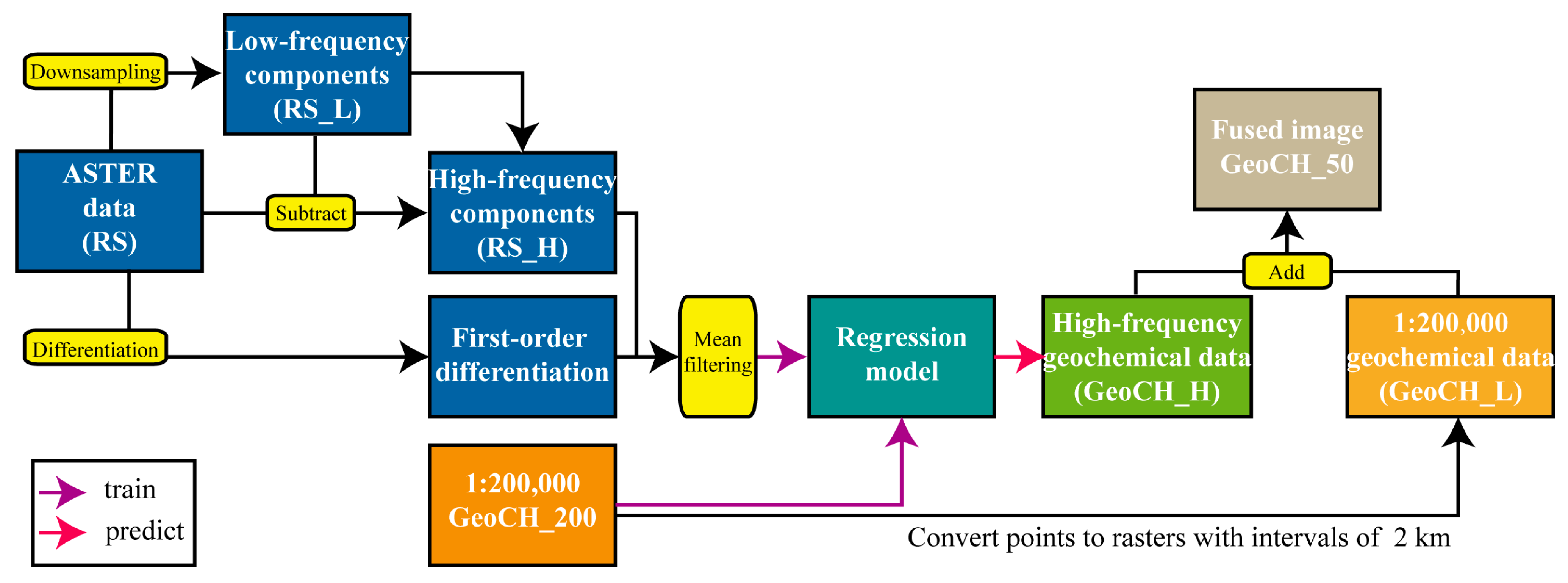
Generally, remote sensing images have higher spatial resolutions because high-frequency information reflects areas where grayscale values change sharply, such as image textures and edges, and low-frequency information reflects areas where image grayscale values change slowly and continuously [50]. Compared with medium-resolution remote sensing images (e.g., Landsat-8 OLI, 30 m; ASTER, 15 m, etc.), the commonly used 1:200,000 water system sediment geochemical data is low-resolution or low-frequency data (the spatial resolution after grid is 2 km). In some studies, a variety of situations makes it impossible to obtain high-precision geochemical data, and to obtain a more detailed spatial distribution of element content and prerequisite geochemical analysis, the method of interpolation (IDW or Kriging method) is generally used to obtain high-resolution geochemical data. However, as mentioned in the first section, neither method is optimal in terms of use and effect. This paper proposes a strategy for integrating remote sensing data with geochemical data by using high-frequency information from remote sensing data to encrypt low-spatial resolution (low-frequency geochemical data). The advantage of this approach is that, on the one hand, the geochemical data are used for the abnormal distribution of elements and their combinations [51,52] in surveys; they are also frequently used to identify mineral combinations or characteristic geological bodies (such as rock masses, ore bodies, strata, etc.) [53,54]. On the other hand, free medium-resolution remote sensing images (spatial resolution) are more readily available, and remote sensing data with SWIR bands can usually reflect the mineral composition and content of features [55], which has a similar function to geochemical data in some ways. For example, alteration information can reflect mineralization information (such as Cu) [56]. Therefore, the integration of remote sensing and geochemical data can solve many of the difficulties caused by the low spatial accuracy of geochemical data in geological research. Some researchers have realized the analysis of Cu element-related information based on ASTER data [57,58]. As mentioned above, the previous remote sensing and geochemical data fusion methods have the disadvantage of fuzzing the spatial details of remote sensing data. In order to make the remote sensing data better serve the improvement of the spatial resolution of geochemical data and prevent it from losing its role in reflecting the mineral composition and content in the geomorphology, a new remote sensing and geochemical data fusion strategy is proposed to meet the above requirements. Figure 3 shows the fusion steps of remote sensing with geochemical data using ASTER data as an example.

Step1: The high-frequency information of remote sensing data is obtained from the remote sensing image (RS) by the Gaussian pyramid decomposition method. The low-frequency information (RS_L) of the remote sensing data is obtained by down-sampling the RS data. The high frequency information (RS_H) of the original RS data can be obtained by subtracting the original data and the RS_L of the remote sensing data. In order to obtain the characteristics of the spectral dimension, the RS data takes the first derivative in the spectral dimension. The obtained spectral first derivative information and high-frequency remote sensing data are used in model training and prediction. Image data has a strong local correlation in space and contains a significant amount of redundant information. In order to prevent redundant information from interfering with the model training process, the training data is compressed with a mean filter with a size of 5 × 5 to smooth the training data and reduce the interference of noise on the model.

Step2: Regression modeling can obtain the relationship between 1:200,000 geochemical data (GeoCH_200) and RS_H data. Linear (linear regression) and non-linear methods (random forests, support vector regression) can be used for the model and allow new geochemical element interpolation data ($\mathrm{GeoCH}\_\mathrm{H}$) can be generated; the process can be represented by Equation (1). Compared with 1:200,000 geochemical data, the generated geochemical data (GeoCH_50) contains more information about spatial details, which belong to geochemical high-frequency information.

2.4. Regression Models

In this paper, two nonlinear machine learning methods of random forest and support vector regression are used to achieve both remote sensing geochemical data fusion (Step2 in Section 2.3) and the regression of RS_H data and geochemical data. The regression model chooses one of the three methods to generate GeoCH_H, and finally obtains the fusion result. In addition, the traditional linear regression-based fusion model is compared with the results of three machine models to verify the effectiveness of the machine model in the data fusion process. For nonlinear machine learning models, in order to achieve the regression of RS_H data and geochemical data, the geochemical data are rounded down to form discrete data when the model is built, and the number of labels of discrete data is n. The regression problem can be converted into n classification problem, so as to realize the RS_H data and geochemical data regression of nonlinear machine learning methods.

2.4.1. Linear

In statistics, linear regression is commonly used to model the relationship between one or more independent variables and a dependent variable [59]. This method is widely used in the study of multivariate geological systems [60]. The principle of linear regression is as follows.

$$\mathrm{Y}=a_1{x}_1+a_2{x}_2+a_3{x}_3+a_4{x}_4+a_5{x}_5+a_6{x}_6+a_7{x}_7+a_8{x}_8+a_9{x}_9+a_{10}{x}_{10}$$

(2)

where x_i (i = 1, 2, …, 10) represents the matrix of DN values of all pixels in the corresponding region of the i-th band of the RS_H data (Figure 3), $x_{10}$ is the first derivative differentiation, a_i (i = 1, 2, …, 10) represents the regression coefficient, and Y represents the measured 1:200,000 geochemical data distribution (Figure 2, red).

2.4.2. Random Forest (RF)

The RF [61] algorithm is one of the most commonly used supervised learning algorithms; it belongs to the Bagging (Bootstrap aggregation) method [62] in integrated learning. The method used for regression analysis consists of two stages: (1) In the model training phase, random forest uses bootstrap sampling to randomly collect multiple different sub-training data sets from the input training data set to sequentially train multiple different classification and regression trees (CART). During training, it is necessary to consider how to select segmentation variables (features) and segmentation points, and how to measure the quality of segmentation variables and segmentation points. For the first problem, it is possible to find the best segmentation variable and segmentation point by separating all the features randomly extracted from each tree and all the values of each feature; for the latter problem, it can be measured by the smaller weighted sum of the impurity (for regression analysis, impurity can be defined using mean squared error-MSE or absolute mean error-MAE) of each child node after segmentation. (2) In the model prediction stage, the RS_H data is put into the RF, and the final predicted result is obtained by taking the average value according to the predicted results of multiple decision trees. The advantages of random forest are mainly reflected in: (1) the classification accuracy is generally better than a single decision tree classifier, provided that the correlation of each decision tree is small; (2) due to the double randomness of samples and features, the model is not easy to fall into overfitting; (3) while classifying the data, the importance score of each feature can also be given to evaluate the role of each feature in the classification. The regression steps of random forest are as follows (Figure 4).

STEP 1: Extract m training samples from all training data with replacement and obtain new n sub-training sets (S1…Sn).

STEP 2: Train a CART with the training set data. During the training process, the segmentation rule of each node is to randomly select k features from all features (different bands of RS data), and select the optimal segmentation point among these k features to divide the left and right subtrees. Through this process, multiple different CART regression trees can be generated.

STEP 3: When predicting, the 9-band remote sensing data is input into the random forest model as an independent variable, and the final prediction result of each CART regression tree is obtained.

STEP 4: Each predication of CART regression tree is averaged to obtain the final prediction result.

2.4.3. Support Vector Regression (SVR)

SVM is a binary classification model [63] that is a learning strategy based on interval maximization. The SVM can be formalized as a problem for solving convex quadratic programming, such as regression problems [64]. The regression steps of SVR are shown in Figure 5.

The training data in the regression problem is $X=\left\{X_1,\cdots ,X_{1643}\right\}$. $X_{\mathrm{n}}$is the ASTER data for this region. $Y=\left\{y_1,\cdots ,y_{1643}\right\}$. $y_{\mathrm{n}}$is the measured geochemical data corresponding to the training data in this area.

If there is a hyperplane in the feature space where the training data is located, the hyperplane can make the distance between any sample point and the hyperplane less than or equal to 1 according to the label.

$$w^{T}X+b=0$$

(3)

$$y_i\left(w^T{X}_i+b\right)\le 1$$

(4)

The above Equation (3) is the decision boundary, $w^T$, b is the coefficient of the decision boundary function, which is used to uniquely determine the decision boundary, so that the sample will be correctly fitted. Equation (4) is the distance from the sample point to the hyperplane. In SVR, it is necessary to ensure that the distance between all sample points and the hyperplane is less than or equal to the point farthest from the hyperplane. $X_i$, $y_i$ is the point farthest from the hyperplane. When the decision boundary satisfies Equations (3) and (4), two parallel hyperplanes can actually be constructed as interval boundaries to judge whether a sample is correctly predicted:

$$w^T{X}_i+b\ge 1$$

(5)

$$w^T{X}_i+b\le -1$$

(6)

The distance between the two interval boundaries is $d=\frac{2}{\left|\left|w\right|\right|}$ Defined as margin, $\left|\left|w\right|\right|$ is the distance from Equations (3)–(5) or (6). Samples located on the interval boundary are called support vectors. SVR allows some samples that are indivisible in linear space to have hypersurfaces in the eigenspace to separate samples. Because of this, nonlinear mapping functions are used to map sample distributions from the original feature space to the higher-dimensional Hilbert space, thereby converting nonlinear problems into linear problems to classify samples. However, the complex form of the mapping function makes it difficult to calculate its inner product, so the kernel method can be used to subtract the computation process [65]. The training sample set X is composed of the first derivative differentiation and RS_H, and the label data Y is geochemical data which sampled by field work. The number of values present in the label data is n.

2.5. Reference of Data Fusion

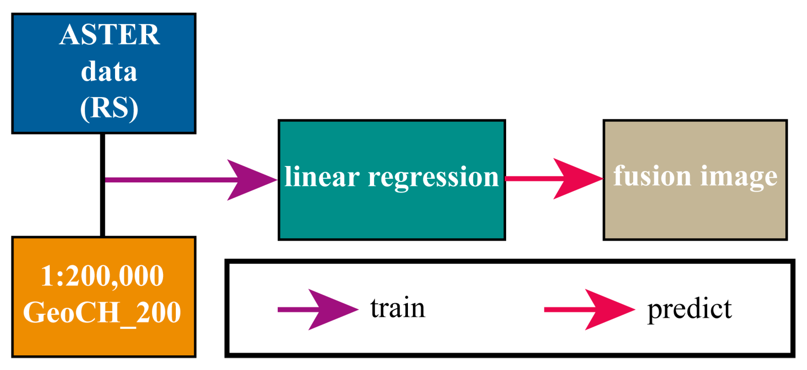
In order to evaluate the quality of the fusion strategy proposed in this paper, linear regression is selected to achieve RS data and geochemical data fusion. This method does not decompose RS data into high- and low-frequency information, but instead uses the DN value of ASTER data as the independent variable and the 1:200,000 geochemical data as the dependent variable to establish a regression model. To distinguish it from the aforementioned linear regression method (in Section 2.4.1), this method is called direct linear regression in the current paper. Comparing the fusion result of direct linear regression with the fusion results of linear regression, RF and SVR can evaluate the effectiveness of the fusion strategy. The direct linear fusion method is shown in Figure 6.

2.6. Evaluation Method

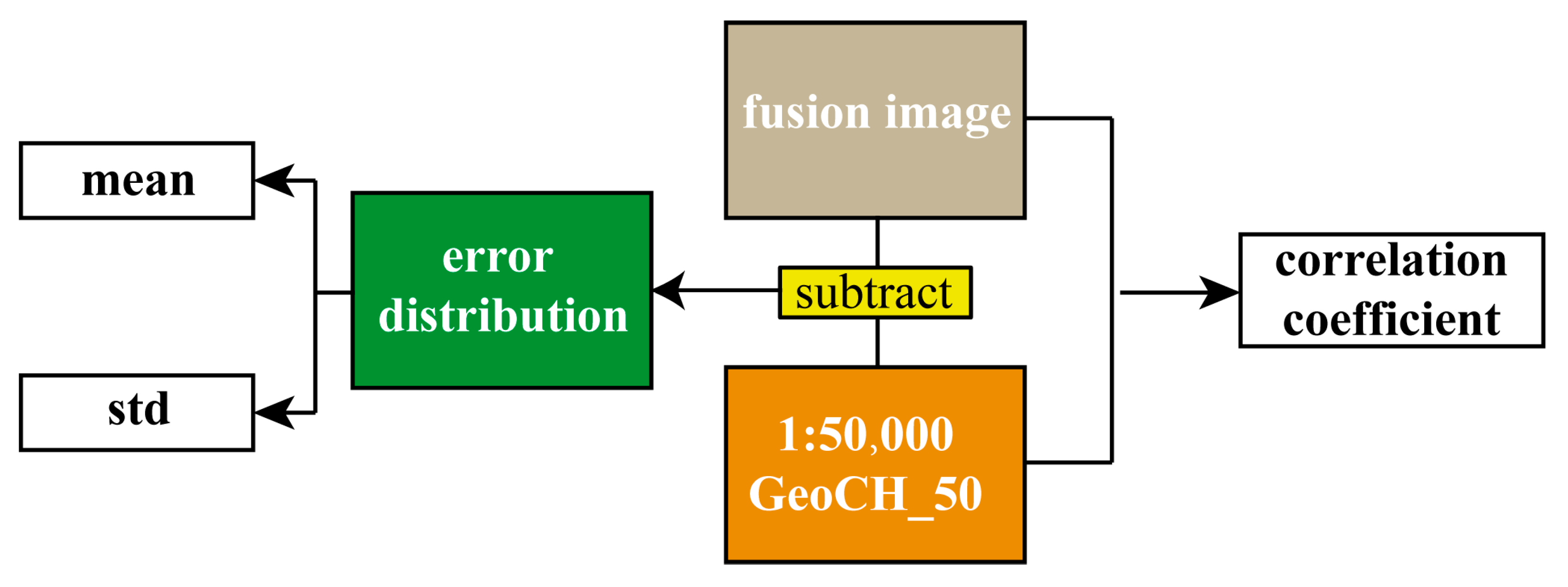
Three indicators of mean, standard deviation (Std), and correlation coefficient are used to evaluate the quality of fusion results. The calculation methods of the three indicators are different. When calculating the mean and Std, firstly, the fusion result should be compared with the 1:50,000 geochemical data (GeoCH_50, Figure 7), and then the mean variance of the error image should be calculated. The mean and Std can measure the degree of difference between the fused image and the GeoCH_50. The correlation coefficient is directly calculated from the GeoCH_50 and the fusion result, which can measure the degree of consistency between the fusion image and the distribution trend of the GeoCH_50. The calculation methods of the three indicators shown in Figure 7.

(1)

Mean

Mean can indicate the overall difference between the fusion result (1:50,000 geochemical data obtained through fusion) and the real geochemical data distribution (original 1:50,000 geochemical data). The predicted results are compared with the original geochemical data, and the smaller the mean value of the difference image is, the smaller the overall deviation between the predicted image and the real geochemical data.

(2)

Standard deviation

Standard deviation indicates how far the fusion results deviate from the real distribution of geochemical data. The smaller the variance of the difference image between the predicted result and the original geochemical data, the smaller the difference between the predicted image and the real geochemical data.

(3)

Correlation coefficient

Correlation coefficients are widely used to measure the degree of correlation between two variables. The correlation coefficient between the fusion result and the 1:50,000 geochemical data is compared with the correlation coefficient between 1:200,000 and 1:50,000 geochemical data (20-5), so as to quantitatively evaluate the similarity between the fusion result and the verification data. The correlation coefficient between two variables is defined as Equation (7).

$$\rho =\frac{cov\left(X,Y\right)}{{\sigma }_X{\sigma }_y}=\frac{E\left[\left(X-\mu x\right)\left(Y-\mu y\right)\right]}{{\sigma }_X{\sigma }_y}$$

(7)

where cov(X, Y) is the covariance of X, Y, X is 1:200,000 geochemical data and Y is 1:50,000 geochemical data. Where ${\sigma }_X$ is the standard deviation of X and ${\sigma }_y$ is the standard deviation of Y.

3. Results

3.1. Fused Results

A total of 1:50,000 geochemical data were selected as validation data to evaluate the results obtained by each fusion method. Fusion experiments are carried out in the Dacaotan area, which is shown in Figure 2 (green). Cu and remote sensing data are used to acquire fusion result by linear regression, random forest and support vector regression methods. The distribution of 1:50,000 geochemical data and 1:200,000 geochemical data is shown in Figure 8. The verification area contains typical geological bodies in this area, as well as Heishan Cu deposits, which can represent the geological characteristics of this area. From the histogram distribution of the two sets of data, although there is a certain degree of difference, the overall distribution is similar. The mean of the 1:50,000 geochemical data is slightly higher than that of the 1:200,000 geochemical data (

Table 1. Statistical results of geochemical data.

Data Type	Mean	Std	Min	Max
1:50,000	26.23	12.90	0.00	63.00
1:200,000	22.86	11.25	3.00	64.00

), indicating that the Cu element in the verification area is more enriched than the entire study area. There is no obvious difference in Std, maximum value and minimum value, indicating that this area can reflect the overall characteristics of the study area.

The fusion results quality of Cu and RS data are evaluated in

Table 2. Statistical results of fusion images.

Method	Mean	Std	Correlation (Geochemical)	Correlation (RS)
Cu
Direct linear	59.07	68.91	0.33	0.13
Linear	4.29	6.70	0.70	0.39
Random forest	3.45	5.04	0.71	0.31
SVR	5.09	5.02	0.72	0.32
20-5	7.22	7.00	0.67	0.24

. The 1:50,000 geochemical data have higher spatial accuracy and more complete information than 1:200,000 geochemical data. The more similar the fusion result is to 1:50,000 geochemical data, the better the fusion method can reflect the distribution of Cu in this area. Therefore, the mean, Std and correlation coefficient between the fusion result and the 1:50,000 geochemical data are compared with the parameters between 1:200,000 geochemical data and 1:50,000 geochemical data (Table 2, 20-5) to quantitatively evaluate the similarity between the fusion result and the verification data. The fusion result is shown in Figure 9.

The mean and Std of direct linear regression are much higher than 20-5, and the correlation coefficient of geochemical and RS are significantly lower than 20-5; at the same time, while the mean and Std of linear regression are lower than 20-5 (Table 2), and the correlation coefficient (geochemical, RS) is higher than 20-5. Taken together, this indicates that the fusion strategy proposed in this paper can improve the quality of 1:200,000 geochemical data, both in terms of space and information richness. The mean and Std of RF and SVR are lower than that of linear regression, while the correlation coefficient (geochemical, RS) is higher than that of linear regression (Table 2), indicating that the nonlinear fusion method can better reflect the geochemical characteristics of the study area.

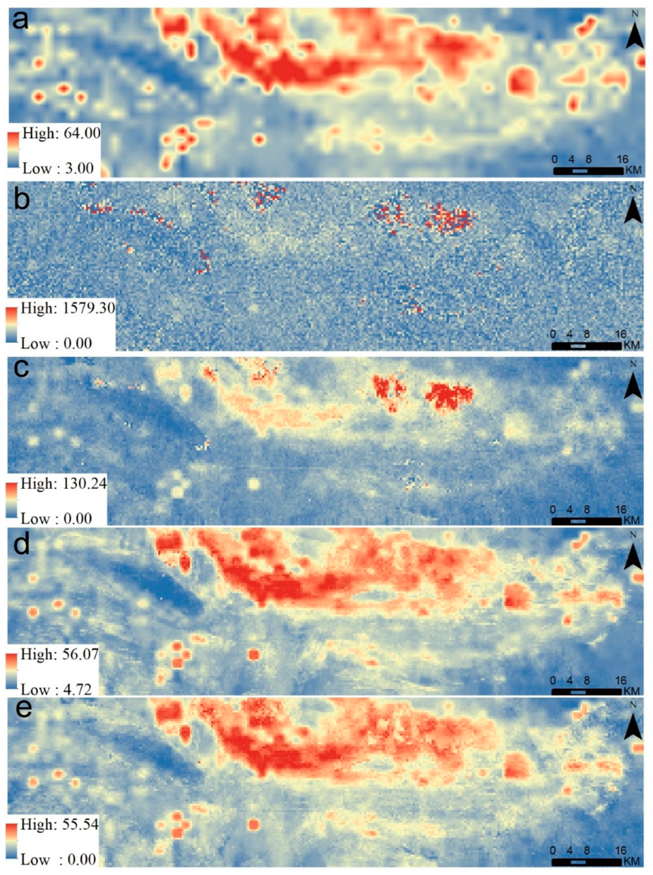
The direct linear regression (Figure 9b) shows a low similarity between the fusion results and the real geochemical elements, and the distribution of Cu element is not reflected clearly in the fusion result. The result fused by linear regression (Figure 9c) shows a higher similarity with true geochemical data, and the distribution of Cu is consistent with the true geochemical data. However, there are still differences between the extreme value distribution and the true geochemical data. Comparing the direct linear regression with the linear regression method, it can be seen that the method proposed in this paper can improve the fusion effect. The result fused by RF (Figure 9d) and SVR (Figure 9e) shows that the distribution of the fusion result is consistent with the true geochemical data. Comparing the fusion result with linear regression, the extreme value is more similar to the real geochemical data.

The direct linear regression method is used as a benchmark to evaluate the performance of each machine learning method proposed in this paper. The value of the mean and Std of the fusion result through direct linear regression is large, indicating that the distribution of the fusion result is quite different from the distribution of true geochemical data. It is difficult to characterize the distribution of geochemical data. The correlation coefficient between the direct regression fusion result and the 1:50,000 data is low (0.33), indicating that the correlation between the fusion result and the 1:50,000 data is not obvious, and is much lower than the correlation coefficient between 1:200,000 geochemical data and the 1:50,000 geochemical data. The correlation coefficient shows that this method cannot effectively obtain information related to geochemical elements from RS data. The correlation coefficient between the fusion result of direct linear regression and RS data is low (0.13), indicating that this method cannot effectively fuse the spatial detail information in RS data.

The mean and Std of fusion results obtained by using the linear regression method of the fusion strategy proposed in this paper is smaller than that of the direct linear regression method, indicating that the fusion strategy proposed in this paper can better reflect the regulation between geochemical data and RS data. The fusion result has a high correlation with the 1:50,000 geochemical data (0.70), which is also higher than the correlation coefficient between the 1:200,000 and 1:50,000 geochemical data (0.67), indicating that the linear regression fusion method can effectively obtain the relevant information of geochemical elements from RS images. The fusion results obtained by this method have the highest correlation coefficient with RS images (0.39), indicating that the linear regression method can reflect the spatial details better than RS images.

The mean and Std of the fusion result obtained by the RF method is slightly smaller than that of the linear regression method. It shows that the RF method can better reflect the regulation between geochemical data and RS data. The fusion results have a higher correlation (0.71) with the 1:50,000 data, which is higher than the correlation coefficient between the 1:200,000 geochemical data and the 1:50,000 geochemical data (0.67), indicating that the RF fusion method can achieve better information about geochemical elements than RS data. The correlation coefficient between the RF fusion result and RS data is lower than that of the linear regression method (0.31), but the difference is small, indicating that the RF method can efficiently add spatial detail information of RS data.

The mean value of the fusion result obtained by using the SVR method is slightly higher than that of the linear regression method, and the Std is smaller than that of the linear regression method, but it is an approximate result. However, it does show that the SVR method can better reflect the regulation between geochemical data and RS data. The fusion result has the highest correlation coefficient (0.72) with the 1:50,000 geochemical data, indicating that the SVR fusion method can obtain the relevant information of geochemical elements from RS data. The correlation coefficient between SVR fusion result and RS data is lower than that of the linear regression method (0.32) and higher than that of the RF method, indicating that the SVR method can efficiently add spatial detail information of RS data on the premise of maintaining the low-frequency information of geochemical data than other methods.

From the perspective of visual interpretation, although the fusion strategy proposed in this paper improves the quality of the 1:200,000 geochemical data, the fusion results still retain most of the distribution characteristics of the 1:200,000 geochemical data. However, there are still differences in the fusion results between linear methods and nonlinear methods. In the fusion results of direct linear regression and linear regression, there is a high value of geochemical data in the upper right corner (Figure 9b,c), which does not exist in the 1:50,000 geochemical data (Figure 9a). In the fusion results of RF and SVR, the high values are basically distributed along the direction from upper left to lower right, which is consistent with the 1:50,000 geochemical data. The fusion results of linear regression and RF are quite different from the 1:50,000 geochemical data. In the fusion results of linear regression, the distribution trend of geochemical elements is different from the 1:5 data, so the mean and Std are higher than 20-5. In the fusion results of RF, the average value is low, but the Std is high, indicating that there are outliers in the fusion results that are different from the 1:50,000 geochemical data, but since there are not many such outliers, they do not affect the distribution of geochemical elements in the fusion results. The mean and Std of the SVR fusion results is low, indicating that the method can reflect the distribution of geochemical data and avoid the interference of irrelevant information in RS data, which has good robustness. In general, the nonlinear methods can better characterize the spatial detail information of RS data and the geochemical element distribution in fusion results.

3.2. Statistical Evaluation on the Fused Results

The fusion results of Cu and RS data using direct regression, linear regression, random forest, and support vector regression methods in the entire study area are shown in the figure below (Figure 10). The fusion results obtained by the direct regression method are different from the distribution of real geochemical elements, and the detailed information in the RS data cannot be well reflected (Figure 10b). The linear regression fusion results (Figure 10c) retain the spatial details of geochemical information and RS data to a certain extent, but the expression of geochemical information is inconsistent with that in Figure 10a, indicating that the linear regression model cannot better characterize the distribution of geochemical elements. The fusion results of the nonlinear methods (Figure 10d,e) are basically consistent with the distribution of real geochemical elements, and the fusion image is clearer.

4. Discussion

This paper uses direct linear regression, linear regression, RF and SVR to fuse RS data and geochemical data. The fusion results of direct linear regression cannot retain the distribution characteristics of geochemical data. Linear regression can preserve the distribution characteristics of geochemical data, which proves the effectiveness of the fusion strategy. However, the fusion results of the linear regression method are still quite different from the 1:50,000 geochemical data, indicating that the linear method cannot fit the RS data and geochemical data well. Nonlinear methods have a better effect on improving the spatial detail of geochemical data. Based on the fusion strategy, the fusion results of various methods can be improved, which proves that the fusion strategy has good robustness. Through visual analysis and judgment of multiple indicators, the SVR fusion method can better achieve the goal of fusion of spatial detail information of RS data and geochemical data.

There is such a phenomenon in the fusion results. When the correlation coefficient between the fusion results and the RS images increases, the Std of the fusion results will increase because when more spatial detail information is added to the fusion result, the result becomes closer to the remote sensing data, and the spatial detail information of the verification data is much smaller than that of the RS data. Compared with the RS data, the 1:50,000 geochemical data is still low-frequency information, so when more high-frequency information is added to the fusion result, it will be less similar to the low-frequency information of geochemical data.

Although the experiment has successfully realized the fusion of high-frequency information of geochemical data and remote sensing data, there are some problems with the implementation of the model, as follows. (1) The parameters of the fusion model are not optimized, and the parameters currently used by the fusion model may not be optimal, meaning that the fusion model can still improve the quality of the fusion results by parameter tuning. (2) The fusion data uses raw data without additional feature engineering, which can make the model run slower or introduce unnecessary noise [66]. In order to obtain more refined fusion results, the following methods can be used in further work. (3) When building a remote sensing-geochemical data fusion model, the best parameters can be examined through hyperparameter search, including the best window size, the best sampling step, etc. Before data fusion, remote sensing data can filter features, such as extracting alteration information; then, based on this information, remote sensing-geochemical data fusion can be achieved to improve the quality of fused images.

5. Conclusions

In practice, low-precision geochemical data has become an important factor restricting the accuracy of related research. The acquisition of high-precision geochemical data requires enormous human, material and financial support, which is quite difficult for studies that have low budgets. According to the characteristics of wide coverage, high precision and cheap acquisition of remote sensing data, this paper proposes a fusion strategy based on geochemical data and remote sensing data. The method can improve the quality of geological work and reduce economic costs in areas with harsh natural conditions. The experimental results show that there is indeed a correlation between the geochemical data and the remote sensing data, and the fusion strategy proposed in this paper can effectively integrate the high-frequency information of the remote sensing data and the geochemical data according to the correlation, allowing the geochemical data to be refined. Under the fusion strategy proposed in this paper, the fusion of remote sensing and geochemistry based on machine learning has achieved good results, which proves the effectiveness of the fusion strategy. The nonlinear methods can add the spatial details of the remote sensing data to the fusion results and maintain the low-frequency information of geochemical elements. The results show that the nonlinear methods can better reflect the distribution characteristics of geochemical data. In the field of geology, the aggregation and distribution of matter is a nonlinear process, and the fusion results better reflect this conclusion. Among the two nonlinear methods, the SVR can better characterize the spatial details in remote sensing data while keeping the distribution of geochemical elements consistent. However, deep learning has replaced traditional methods with superior results on problems such as classification, detection, etc. Therefore, it is worth attempting to use deep learning methods to integrate remote sensing data and geochemical data.

References

1. Doran, J.W.; Coleman, D.C.; Bezdicek, D.; Stewart, B. Defining Soil Quality for a Sustainable Environment; Food and Agriculture Organization of the United Nations: Rome, Italy, 1994. [Google Scholar]
2. West, T.O.; Post, W.M. Soil organic carbon sequestration rates by tillage and crop rotation: A global data analysis. Soil Sci. Soc. Am. J. 2002, 66, 1930–1946. [Google Scholar] [CrossRef]
3. Beus, A.A.; Grigorian, S.V. Geochemical Exploration Methods for Mineral Deposits. 1977. Available online: https://www.osti.gov/biblio/7211784 (accessed on 23 April 2021).
4. Krishnakumar, S.; Ramasamy, S.; Chandrasekar, N.; Peter, T.S.; Godson, P.S.; Gopal, V.; Magesh, N. Spatial risk assessment and trace element concentration in reef associated sediments of Van Island, southern part of the Gulf of Mannar, India. Mar. Pollut. Bull. 2017, 115, 444–450. [Google Scholar] [PubMed]
5. Krishnakumar, S.; Ramasamy, S.; Peter, T.S.; Godson, P.S.; Chandrasekar, N.; Magesh, N. Geospatial risk assessment and trace element concentration in reef associated sediments, northern part of Gulf of Mannar biosphere reserve, Southeast Coast of India. Mar. Pollut. Bull. 2017, 125, 522–529. [Google Scholar]
6. Xie, X.; Cheng, H. Sixty years of exploration geochemistry in China. J. Geochem. Explor. 2014, 139, 4–8. [Google Scholar]
7. Wang, Z.; Zuo, R.; Liu, H. Lithological mapping based on fully convolutional network and multi-source geological data. Remote Sens. 2021, 13, 4860. [Google Scholar]
8. Yang, N.; Zhang, Z.; Yang, J.; Hong, Z.; Shi, J. A convolutional neural network of GoogLeNet applied in mineral prospectivity prediction based on multi-source geoinformation. Nat. Resour. Res. 2021, 30, 3905–3923. [Google Scholar]
9. Campbell, J.B.; Wynne, R.H. Introduction to Remote Sensing; Guilford Press: New York, NY, USA, 2011. [Google Scholar]
10. Gupta, R.P. Remote Sensing Geology; Springer: Berlin/Heidelberg, Germany, 2017. [Google Scholar]
11. Tappert, M.C.; Rivard, B.; Giles, D.; Tappert, R.; Mauger, A. The mineral chemistry, near-infrared, and mid-infrared reflectance spectroscopy of phengite from the Olympic Dam IOCG deposit, South Australia. Ore Geol. Rev. 2013, 53, 26–38. [Google Scholar]
12. Kokaly, R.; Graham, G.E.; Hoefen, T.M.; Kelley, K.D.; Johnson, M.R.; Hubbard, B.E.; Buchhorn, M.; Prakash, A. Multiscale hyperspectral imaging of the Orange Hill Porphyry Copper Deposit, Alaska, USA, with laboratory-, field-, and aircraft-based imaging spectrometers. Proc. Explor. 2017, 17, 923–943. [Google Scholar]
13. Meyer, J.M.; Kokaly, R.F.; Holley, E. Hyperspectral remote sensing of white mica: A review of imaging and point-based spectrometer studies for mineral resources, with spectrometer design considerations. Remote Sens. Environ. 2022, 275, 113000. [Google Scholar]
14. Swayze, G.A.; Clark, R.N.; Pearson, R.M.; Livo, K.E. Mapping Acid-Generating Minerals at the California Gulch Superfund Site in Leadville, Colorado Using Imaging Spectroscopy; NASA: Washington, DC, USA, 1996. [Google Scholar]
15. Kopačková-Strnadová, V.; Rapprich, V.; McLemore, V.; Pour, O.; Magna, T. Quantitative estimation of rare earth element abundances in compositionally distinct carbonatites: Implications for proximal remote-sensing prospection of critical elements. Int. J. Appl. Earth Obs. Geoinf. 2021, 103, 102423. [Google Scholar] [CrossRef]
16. Huadong, G.; Pinliang, D. Integrated MSS-SAR-SPOT-geophysical and geochemical data for exploration geology in Yeder area. Adv. Space Res. 1992, 12, 27–30. [Google Scholar] [CrossRef]
17. Fazliani, H.; Kamkar-Rouhani, A.; Arab-Amiri, A. Integration and analysis of geological, geochemical and remote sensing data of south of Neyshabur using principal component analysis. Int. J. Min. Geo-Eng. 2021, 55, 161–170. [Google Scholar]
18. Marjanović, M.; Kovačević, M.; Bajat, B.; Voženílek, V. Landslide susceptibility assessment using SVM machine learning algorithm. Eng. Geol. 2011, 123, 225–234. [Google Scholar]
19. Rodriguez-Galiano, V.; Sanchez-Castillo, M.; Chica-Olmo, M.; Chica-Rivas, M. Machine learning predictive models for mineral prospectivity: An evaluation of neural networks, random forest, regression trees and support vector machines. Ore Geol. Rev. 2015, 71, 804–818. [Google Scholar]
20. Zuo, R. Machine learning of mineralization-related geochemical anomalies: A review of potential methods. Nat. Resour. Res. 2017, 26, 457–464. [Google Scholar] [CrossRef]
21. Lucey, P.G.; Blewett, D.T.; Hawke, B.R. Mapping the FeO and TiO2 content of the lunar surface with multispectral imagery. J. Geophys. Res. Planets 1998, 103, 3679–3699. [Google Scholar] [CrossRef]
22. Wang, Z.; Zuo, R.; Jing, L. Fusion of geochemical and remote-sensing data for lithological mapping using random forest metric learning. Math. Geosci. 2021, 53, 1125–1145. [Google Scholar] [CrossRef]
23. Moradpour, H.; Rostami Paydar, G.; Feizizadeh, B.; Blaschke, T.; Pour, A.B.; Valizadeh Kamran, K.; Muslim, A.M.; Hossain, M.S. Fusion of ASTER satellite imagery, geochemical and geology data for gold prospecting in the Astaneh granite intrusive, West Central Iran. Int. J. Image Data Fusion 2022, 13, 71–94. [Google Scholar] [CrossRef]
24. Contreras, C.; Khodadadzadeh, M.; Tusa, L.; Loidolt, C.; Tolosana-Delgado, R.; Gloaguen, R. Geochemical and Hyperspectral Data Fusion for Drill-Core Mineral Mapping. In Proceedings of the 2019 10th Workshop on Hyperspectral Imaging and Signal Processing: Evolution in Remote Sensing (WHISPERS), Amsterdam, The Netherlands, 24–26 September 2019. [Google Scholar]
25. Jiang, L.; Xing, L.; Liang, Y.; Pan, J.; Liang, L.-H.; Huang, J.-C. Anomalies information extraction from geochemical data and remote sensing fusion. J. Jilin Univ. (Earth Sci. Ed.) 2011, 41, 932–936. [Google Scholar]
26. Li, Z.; Zhang, X.; Zhu, R.; Zhang, Z.; Weng, Z. Integrating data-to-data correlation into inverse distance weighting. Comput. Geosci. 2020, 24, 203–216. [Google Scholar]
27. Mao, J.; Pirajno, F.; Zhang, Z.; Chai, F.; Yang, J.; Wu, H.; Chen, S.; Cheng, S.; Zhang, C. Late Variscan post-collisional Cu-Ni sulfide deposits in East Tianshan and Altay in China: Principal characteristics and possible relationship with mantle plume. Acta Geol. Sin. 2006, 80, 925–942. [Google Scholar]
28. Windley, B.; Allen, M.; Zhang, C.; Zhao, Z.; Wang, G. Paleozoic accretion and Cenozoic redeformation of the Chinese Tien Shan range, central Asia. Geology 1990, 18, 128–131. [Google Scholar] [CrossRef]
29. Şengör, A.; Natal’In, B.; Burtman, V. Evolution of the Altaid tectonic collage and Palaeozoic crustal growth in Eurasia. Nature 1993, 364, 299–307. [Google Scholar] [CrossRef]
30. Jahn, B.-m.; Windley, B.; Natal’in, B.; Dobretsov, N. Phanerozoic continental growth in Central Asia. J. Asian Earth Sci. 2004, 5, 599–603. [Google Scholar]
31. Xiao, W.-J.; Zhang, L.-C.; Qin, K.-Z.; Sun, S.; Li, J.-L. Paleozoic accretionary and collisional tectonics of the Eastern Tianshan (China): Implications for the continental growth of central Asia. Am. J. Sci. 2004, 304, 370–395. [Google Scholar] [CrossRef]
32. Qin, K.; Sun, S.; Li, J.; Fang, T.; Wang, S.; Liu, W. Paleozoic epithermal Au and porphyry Cu deposits in North Xinjiang, China: Epochs, features, tectonic linkage and exploration significance. Resour. Geol. 2002, 52, 291–300. [Google Scholar] [CrossRef]
33. Xiao, W.; Han, C.; Yuan, C.; Sun, M.; Lin, S.; Chen, H.; Li, Z.; Li, J.; Sun, S. Middle Cambrian to Permian subduction-related accretionary orogenesis of Northern Xinjiang, NW China: Implications for the tectonic evolution of central Asia. J. Asian Earth Sci. 2008, 32, 102–117. [Google Scholar] [CrossRef]
34. Long, L.; Wang, J.; Wang, Y.; Deng, X.; Mao, Q.; Sun, Y.; Sun, Z.; Zhang, Z. Metallogenic regularity and metallogenic model of the paleo arc-basin system in eastern Tianshan. Acta Petrol. Sin. 2019, 35, 3161–3188. [Google Scholar]
35. Mao, Q.; Yu, M.; Xiao, W.; Windley, B.F.; Li, Y.; Wei, X.; Zhu, J.; Lü, X. Skarn-mineralized porphyry adakites in the Harlik arc at Kalatage, E. Tianshan (NW China): Slab melting in the Devonian-early Carboniferous in the southern Central Asian Orogenic Belt. J. Asian Earth Sci. 2018, 153, 365–378. [Google Scholar]
36. Zhang, Z.; Xiao, W.; Zheng, X.; Yang, G.; Gao, J. Composition, structure and the late Paleozoic evolution of Kanggurtag structural belt in eastern Tianshan. Miner. Explor. 2021, 12, 1530–1538. [Google Scholar]
37. Wang, J.; Wang, Y.; He, Z. Ore deposits as a guide to the tectonic evolution in the East Tianshan Mountains, NW China. Geol. China 2006, 33, 461–469. [Google Scholar]
38. Xiao, W.; Windley, B.F.; Allen, M.B.; Han, C. Paleozoic multiple accretionary and collisional tectonics of the Chinese Tianshan orogenic collage. Gondwana Res. 2013, 23, 1316–1341. [Google Scholar] [CrossRef]
39. Rowan, L.C.; Mars, J.C. Lithologic mapping in the Mountain Pass, California area using advanced spaceborne thermal emission and reflection radiometer (ASTER) data. Remote Sens. Environ. 2003, 84, 350–366. [Google Scholar] [CrossRef]
40. Gabr, S.; Ghulam, A.; Kusky, T. Detecting areas of high-potential gold mineralization using ASTER data. Ore Geol. Rev. 2010, 38, 59–69. [Google Scholar]
41. Shirazi, A.; Hezarkhani, A.; Beiranvand Pour, A.; Shirazy, A.; Hashim, M. Neuro-Fuzzy-AHP (NFAHP) Technique for Copper Exploration Using Advanced Spaceborne Thermal Emission and Reflection Radiometer (ASTER) and Geological Datasets in the Sahlabad Mining Area, East Iran. Remote Sens. 2022, 14, 5562. [Google Scholar]
42. Kurata, K.; Yamaguchi, Y. Integration and visualization of mineralogical and topographical information derived from ASTER and DEM data. Remote Sens. 2019, 11, 162. [Google Scholar] [CrossRef]
43. Goshtasby, A. Registration of images with geometric distortions. IEEE Trans. Geosci. Remote Sens. 1988, 26, 60–64. [Google Scholar]
44. Chavez, P.S. Image-based atmospheric corrections-revisited and improved. Photogramm. Eng. Remote Sens. 1996, 62, 1025–1035. [Google Scholar]
45. Department of Geology and Mineral Resources Survey and Technology Division. Regional Geochemistry Exploration Specifications—Proportional Scale 1:200,000; National Standardization Technical Committee of Geology and Mineral Resources Technical Committee Geophysical and Geochemical: Beijing China, 1996. [Google Scholar]
46. Xuejing, X.; Xuzhan, M.; Tianxiang, R. Geochemical mapping in China. J. Geochem. Explor. 1997, 60, 99–113. [Google Scholar] [CrossRef]
47. Zhuang, D.; Liu, T.; Hu, J.; Wang, X. The review and prospect of regional geochemical exploration in Xinjiang. Geophys. Geochem. Explor. 2003, 27, 425–427. [Google Scholar]
48. Wang, H.; Yuan, Z.; Cheng, Q.; Zhang, S.; Sadeghi, B. Geochemical anomaly definition using stream sediments landscape modeling. Ore Geol. Rev. 2022, 142, 104715. [Google Scholar] [CrossRef]
49. Manyika, J.; Durrant-Whyte, H. Data Fusion and Sensor Management: A Decentralized Information-Theoretic Approach; Prentice Hall PTR: Hoboken, NJ, USA, 1995. [Google Scholar]
50. Jing, L.; Cheng, Q. A technique based on non-linear transform and multivariate analysis to merge thermal infrared data and higher-resolution multispectral data. Int. J. Remote Sens. 2010, 31, 6459–6471. [Google Scholar] [CrossRef]
51. Grunsky, E.; Agterberg, F. Spatial and multivariate analysis of geochemical data from metavolcanic rocks in the Ben Nevis area, Ontario. Math. Geol. 1988, 20, 825–861. [Google Scholar]
52. Reimann, C.; Garrett, R.G. Geochemical background—Concept and reality. Sci. Total Environ. 2005, 350, 12–27. [Google Scholar] [CrossRef] [PubMed]
53. McLennan, S.M.; Taylor, S.; Kröner, A. Geochemical evolution of Archean shales from South Africa. I. The Swaziland and Pongola Supergroups. Precambrian Res. 1983, 22, 93–124. [Google Scholar] [CrossRef]
54. Cheng, Q.; Agterberg, F.; Ballantyne, S. The separation of geochemical anomalies from background by fractal methods. J. Geochem. Explor. 1994, 51, 109–130. [Google Scholar] [CrossRef]
55. Povarennykh, A. The use of infrared spectra for the determination of minerals. Am. Mineral. 1978, 63, 956–959. [Google Scholar]
56. Wu, M.; Zhou, K.; Wang, Q.; Wang, J. Mapping hydrothermal zoning pattern of porphyry Cu deposit using absorption feature parameters calculated from ASTER data. Remote Sens. 2019, 11, 1729. [Google Scholar] [CrossRef]
57. Chattoraj, S.L.; Prasad, G.; Sharma, R.U.; van der Meer, F.D.; Guha, A.; Pour, A.B. Integration of remote sensing, gravity and geochemical data for exploration of Cu-mineralization in Alwar basin, Rajasthan, India. Int. J. Appl. Earth Obs. Geoinf. 2020, 91, 102162. [Google Scholar] [CrossRef]
58. Karimpour, M.H.; Mazhari, N.; Shafaroudi, A.M. Discrimination of different erosion levels of porphyry Cu deposits using ASTER image processing in eastern Iran: A case study in the Maherabad, Shadan, and Chah Shaljami Areas. Acta Geol. Sin.-Engl. Ed. 2014, 88, 1195–1213. [Google Scholar]
59. Aiken, L.S.; West, S.G.; Reno, R.R. Multiple Regression: Testing and Interpreting Interactions; Sage: Thousand Oaks, CA, USA, 1991. [Google Scholar]
60. Chung, C.-J.F.; Fabbri, A.G.; Westen, C.J.V. Multivariate regression analysis for landslide hazard zonation. In Geographical Information Systems in Assessing Natural Hazards; Springer: Berlin/Heidelberg, Germany, 1995; pp. 107–133. [Google Scholar]
61. Breiman, L. Random forests. Mach. Learn. 2001, 45, 5–32. [Google Scholar]
62. Breiman, L. Bagging predictors. Mach. Learn. 1996, 24, 123–140. [Google Scholar]
63. Burges, C.J. A tutorial on support vector machines for pattern recognition. Data Min. Knowl. Discov. 1998, 2, 121–167. [Google Scholar] [CrossRef]
64. Shevade, S.K.; Keerthi, S.S.; Bhattacharyya, C.; Murthy, K.R.K. Improvements to the SMO algorithm for SVM regression. IEEE Trans. Neural Netw. 2000, 11, 1188–1193. [Google Scholar] [CrossRef] [PubMed] [Green Version]
65. Soentpiet, R. Advances in Kernel Methods: Support Vector Learning; MIT Press: Cambridge, MA, USA, 1999. [Google Scholar]
66. Yu, L.; Liu, H. Feature selection for high-dimensional data: A fast correlation-based filter solution. In Proceedings of the 20th International Conference on Machine Learning (ICML-03), Washington, DC, USA, 21–24 August 2003; pp. 856–863. [Google Scholar]
Figure 1. Geographical location and geological setting of the study area.
Remotesensing 15 00930 g001
Figure 2. Geochemical data and remote sensing data in the study area.
Remotesensing 15 00930 g002
Figure 3. Flowchart showing the fusion process of geochemical and remote sensing data.
Remotesensing 15 00930 g003
Figure 4. Sketch diagram of random forest regression model (Orange dots represent nodes that have been activated by samples. Blue dots represent nodes that have not been activated by samples).
Remotesensing 15 00930 g004
Figure 5. Sketch diagram of support vector regression (Green dots and blue dots are both samples. Samples. Blue dots are samples on the interval boundaries).
Remotesensing 15 00930 g005
Figure 6. Direct linear fusion method.
Remotesensing 15 00930 g006
Figure 7. Evaluation methods.
Remotesensing 15 00930 g007
Figure 8. distribution of geochemical data. (a) 1:200,000 geochemical data, Cu; (b) 1:50,000 geochemical data, Cu.
Remotesensing 15 00930 g008
Figure 9. Cu fusion results ((a) 1:50,000 geochemical data; (b) direct linear regression; (c) linear regression; (d) random forest; (e) support vector regression).
Remotesensing 15 00930 g009
Figure 10. Cu fusion results ((a) 1:200,000 geochemical data; (b) Direct regression; (c) linear regression; (d) random forest; (e) support vector regression).
Remotesensing 15 00930 g010