Construction of Remote Sensing Indices Knowledge Graph (RSIKG) Based on Semantic Hierarchical Graph

Abstract

Remote sensing indices are widely used in various fields of geoscience research. However, there are limits to how effectively the knowledge of indices can be managed or analyzed. One of the main problems is the lack of ontology models and research on indices, which makes it difficult to acquire and update knowledge in this area. Additionally, there is a lack of techniques to analyze the mathematical semantics of indices, making it difficult to directly manage and analyze their mathematical semantics. This study utilizes an ontology and mathematical semantics integration method to offer a novel knowledge graph for a remote sensing index knowledge graph (RSIKG) so as to address these issues. The proposed semantic hierarchical graph structure represents the indices of knowledge with an entity-relationship layer and a mathematical semantic layer. Specifically, ontologies in the entity-relationship layer are constructed to model concepts and relationships among indices. In the mathematical semantics layer, index formulas are represented using mathematical semantic graphs. A method for calculating similarity for index formulas is also proposed. The article describes the entire process of building RSIKG, including the extraction, storage, analysis, and inference of remote sensing index knowledge. Experiments provided in this article demonstrate the intuitive and practical nature of RSIKG for analyzing indices knowledge. Overall, the proposed methods can be useful for knowledge queries and the analysis of indices. And the present study lays the groundwork for future research on analysis techniques and knowledge processing related to remote sensing indices.

1. Introduction

Remote sensing indices are used to characterize surface features or physical quantities. They are produced from mathematical operations on reflectance or radiance values in different spectral bands of remote sensing data. Remote sensing indices, such as vegetation indices [1], are applied in a wide range of fields, including forestry [2], soil [3,4], and water quality [5]. In recent years, there has been an increasing interest in developing remote sensing indices using multiple data sources and novel technologies [6,7,8,9].

Existing research recognizes the critical role of knowledge management and the utilization of models for scientific research [10]. However, much less is known about how to effectively manage and utilize indices [11]. Although some studies have developed indices repositories to integrate and manage indices, management of indices-related resources and knowledge remains insufficient. The major limitation of existing repositories is the lack of appropriate representation of indices. Current research mostly depends on traditional database models to process and store index information. The major drawback of this method is that it reduces natural links, such as similarities, that exist between indices [12,13]. It could restrict the efficiency of identifying optimal indices for applications and the discovery of new knowledge.

Currently, emerging technologies, such as artificial intelligence, can assist scientists in managing and obtaining new knowledge from massive amounts of data and literature more effectively [14]. Knowledge graphs (KG) [15], a method for representing knowledge in terms of entities, attributes, and relationships, have gained increasing interest in recent years. In the field of remote sensing, KGs are primarily employed for extracting and organizing concepts from diverse and heterogeneous data sources [16], integrating and managing data resources [17], aiding tasks such as scene classification [18], and semantic segmentation [19] in remote sensing image interpretation [20]. By linking external heterogeneous information, KGs can also contribute to representation learning and ontology reasoning for crop identification [21], disaster prediction [22], oil spill detection [23], etc. To the best of our knowledge, however, there is no published KG for remote sensing indices. Existing KGs are unsatisfactory because they are not designed to represent remote sensing indices, and they are incapable of analyzing and managing the relationships and mathematical semantics among indices.

To address the aforementioned issues, a method named remote sensing indices knowledge graph (RSIKG) and its construction approach are proposed. This represents an area that has not been explored in current research on remote sensing or geographical KGs. Specifically, the main contributions of this article include the following:

• A remote sensing index knowledge graph (RSIKG) is proposed. The concepts and relationships of remote sensing indices are modeled as ontologies, and they are mapped to graph databases to construct RSIKG.
• A knowledge representation method is developed for remote sensing indices. It adopts a semantic hierarchical graph structure to represent the remote sensing index graph using two layers: The entity-relationship layer and the mathematical semantic layer. The former primarily models the related concepts and their relationships, while the latter represents and analyzes the mathematical semantics of the index formula.
• A complete mathematical semantic processing pipeline for remote sensing indices is presented. It includes the extraction of remote sensing index formulas, the abstraction modeling of semantics, and the construction of mathematical semantic graphs. In addition, a method for calculating the index similarity of mathematical semantic graphs is also proposed.

The remaining sections are organized as follows: The following section provides an overview of relevant resources on remote sensing indices and related work on geographic and remote sensing KGs. Section 3 outlines the concept and theoretical foundation of RSIKG, presenting the entity-relationship layer and mathematical semantics layer of the semantic hierarchical graph. Subsequently, Section 4 details the methodology for constructing RSIKG, encompassing knowledge representation, knowledge acquisition, and knowledge inference. Section 5 discusses the methods and applications. Finally, Section 6 summarizes the key findings and outlines future directions for research.

2. Related Work

2.1. The Existing Remote Sensing Index Resources

To facilitate the selection and computation of remote sensing indices, various software tools and repositories offer abundant resources and functionalities. This section introduces common resources, including data products, tools, and repositories for remote sensing indices (see

Table 1. A categorization for remote sensing indices resources.

Category	Typical Resources	Advantages	Disadvantages in Resources Management
Data products	MODIS, Landsat, Sentinel, AVHRR, etc.	(a) Data ready to use, no need for calculation (b) Various spatial and temporal scales	(a) Resources fragmentation (b) Lack of standardization and reference information
Platform software	ArcGIS Pro 3.2 [24], ENVI 5.7 [25], etc.	(a) Built-in index functions (b) Integrated with various processing and analysis tools	(a) Limited interoperability and expandability (b) Lack of index-related metadata
Cloud-based platform	Google Earth Engine (GEE) [26]	(a) Extensive related resources and a rich set of tools for index analysis (b) Computational capacity	(a) Steep learning curve (b) Limited interoperability and expandability
Specific index calculation tools	ARTMO [27], ExtractEO [28], Remote Sensing Indices Derivation Tool [29]	(a) Easy to use (b) Designed specifically for calculating indices	(a) Limited scope (b) Lack of integration (c) Limited standardization and documentation (d) Lack of index-related metadata
Index databases	Index DataBase (IDB) [30]	(a) Comprehensive collection of indices, includes information on sensor compatibility	(a) Outdated information (b) Limited searchability (c) Lack of expandability
Standardized catalog of indices	Awesome Spectral Indices (ASI) [11]	(a) Machine-readable format, easy to update (b) Connection to related resources	(a) Limited scope and searchability

).

As shown in Table 1, the common resources of remote sensing indices are divided into six categories. Researchers and users can directly use the data products of indices without the need for computation. Nevertheless, the variety of data products is caused by various data sources, developers, and domains. It also leads to the absence of data product standardization. In addition, the spectral information of sensors and their resolution vary depending on the field. Unfortunately, the calculation, formats, and application scenarios of indices lack unified specifications or reference information, which makes it challenging to fully understand data products for non-expert users. A possible solution is to develop a tool that can provide universal metadata for indices. Researchers or users would then be able to determine whether an index could be conducted with the necessary resolution or spectral information.

Platform software can help researchers calculate their own indices when existing data products do not meet their needs. Numerous index functions are implemented by well-known platform software such as ArcGIS [24] and ENVI [25] through their built-in band computation. However, only a few common indices are available on these platforms. Additionally, platform software does not offer enough relevant metadata to assist users in locating and comprehending the requirements of indices.

This issue has been partially resolved by cloud-based platforms by integrating big data storage and computing capacity. As the most prevalent cloud-based geospatial science platform, Google Earth Engine (GEE) [26] provides extensive remote sensing data and a rich set of tools for index analysis. It significantly reduces the barriers to entry for remote sensing research [31]. However, while platform software can calculate common indices, it is not keeping up with the rate at which index development grows. Furthermore, the indices in platform software are deficient in metadata and do not support knowledge management. While platform software provides certain APIs [32] to help with the creation of extension applications, each index in applications is based on their own specific implementation code. Therefore, support for certain and relatively recent sensor data and indices is typically limited in the platform software.

There are also several specially designed computational tools for calculating new indices. They could be complementary to platform software. For example, Rivera et al. [27] developed the Automated Radiative Transfer Models Operator (ARTMO) package. ARTMO is a spectral index evaluation tool based on MATLAB [33]. ExtractEO, developed by SERTIT (https://sertit.unistra.fr/, accessed on 22 August 2023), is a remote sensing index computation tool flow for reading optical and SAR satellite data [28]. It can load and overlay bands, clouds, DEM, and spectral indices in a sensor-independent manner. The Remote Sensing Indices Derivation Tool is an open-source program for calculating indices [29]. It processes data from various satellite sensors, enabling the calculation of multiple indices for vegetation, water bodies, etc. Since they were designed for particular data or indices, it is obvious that their functionality is limited and may not satisfy needs. Moreover, because they were created separately, there is a lack of interoperability between them. They frequently lack index-related metadata collection and management. As a result, it is difficult for users to understand the calculations, data formats, and research scenarios of indices.

Researchers will encounter difficulties when querying and analyzing indices due to the wide variety and dispersed distribution of resources. This issue has not been adequately addressed by the aforementioned tools. A tool that unifies the scattered data and information of indices is needed. The Index DataBase (IDB), developed in [30], is a professional database for satellite sensors and indices. It provides guidance information for indices applications [34]. IDB covers over 500 indices from various domains. Users can search for indices with keywords or the type of sensor and index on the IDB website.

However, the IDB’s most recent records only go back to 2011, which means they lag behind the developments in indices. Meanwhile, IDB lacks technologies to facilitate rapid data parsing and construction. These issues pose challenges for index updates. Recently, Montero et al. [11] introduced the “Awesome Spectral Indices” (ASI), a standardized catalog of spectral indices for earth science. ASI offers a rich index catalog that is machine-readable and linked to a Python library. Each ASI index comes with a long list of properties, including the name, formula, and source references. The user community has the flexibility to extend ASI.

In summary, common sources for multi-source information about indices are limited, apart from ASI and IDB. IDB and ASI lack a standard format and are built on specific environments and dependencies. The relationships between indices and concepts, as well as the semantic relationships between indices, are difficult to represent for all resources, particularly in the mathematical semantics of index formulas.

2.2. Remote Sensing Knowledge Graph

KG provides a new approach for processing and analyzing remote sensing data. It connects entities, attributes, and relationships in remote sensing data to form a structured knowledge network, which would help in the comprehension and application of remote sensing knowledge [16]. Leveraging the rich semantic information in KG can improve the efficiency and accuracy of remote sensing image interpretation. Currently, research on remote sensing KG is primarily focused on the following aspects (

Table 2. The main aspect of the remote sensing knowledge graphs.

Approach	Description
Knowledge graph integration	Utilizing KGs to integrate concepts and knowledge from multiple heterogeneous sources.
Deep learning and ontology reasoning	Integrating deep learning in remote sensing with ontology reasoning techniques from KGs.
Integrating diverse information	Integrating diverse information beyond remote sensing for specific domain problems.

).

The first method is knowledge graph integration. It involves using KG to integrate concepts and knowledge from disparate sources. KG achieves semantic consistency and interoperability by mapping heterogeneous remote sensing data into a unified conceptual space. Abburu and Dube [17] present an ontology-based approach for satellite data management and searching. It supports queries related to ontology concepts, sub-concepts, and concept hierarchies, thereby improving the efficiency and accuracy of queries. With large-scale, heterogeneous, diverse, and dynamically updated geospatial and remote sensing data, Hao et al. [16] built a KG for surveying and remote sensing applications using the ontology-integration approach. Experimental validation demonstrated the effectiveness and visualization capabilities of the KG, highlighting its utility in surveying and remote sensing.

The second approach combines deep learning in remote sensing with ontology reasoning techniques derived from KGs [20], resulting in complementary and better connections between data-driven and knowledge-guided methods. Li et al. [18] optimized the effectiveness of zero-shot and generalized zero-shot classification in remote sensing image scenes using a remote sensing KG. They created a remote sensing KG with 70 different scene categories and linkages, yielding semantic vectors that were then input into a deep network model. This approach aligned the visual features with semantics in the KG, consequently solving the zero-shot issue in remote sensing scene classification. This technique can be applied to semantic segmentation [19] to solve the issue of different segmentation objects with similar spectra [35].

KGs can integrate diverse information to solve specific domain problems. By combining prior information with remote sensing data, KGs improve the predictive capabilities of remote sensing models. Zhao et al. [21] built an optimal feature KG for crop type identification based on prior knowledge. The method can automatically identify optimal feature combinations in the crop recognition model to improve accuracy. Ge et al. [22] proposed a disaster prediction KG by integrating remote sensing data, relevant geographical data, and expert knowledge in disaster analysis. Liu et al. [23] presented a KG-based oil spill inference method. It integrated various oil spill locations extracted from remote sensing images, vector data, text, and atmospheric-oceanic models.

2.3. The Semantic Representation of Mathematical Formulas and Knowledge Graphs

Mathematical formulas are the core information in remote sensing indices and are closely related to KGs (see

Table 3. Relationships between mathematical formulas and knowledge graphs.

Relationships	Description
Mathematical formulas as KGs	Mathematical formulas can be viewed as a special case of KGs, representing relationships and attributes of modeling systems.
KGs for representing mathematical concepts	KGs can be used to express and manage mathematical concepts and equations, facilitating their organization and comprehension.
Semantic reasoning for mathematical formulas	Semantic reasoning models based on KGs can be used to map the semantics of equations onto the KG.

). Mathematical models, which simplify reality, are frequently used to represent complex systems and phenomena. It is similar to maps that show relationships and patterns within a system [36].

Some researchers argue that mathematical formulas are a form of KG [37]. They consider formulas as a special case of KG [38], because formulas satisfy the definition of KGs that represent the relationships and attributes of modeling systems [39]. Therefore, building KGs using formulas [40] could be a manner of semi-automatically developing and manipulating graphs, with mathematical semantics used to identify concepts within the graph [41].

In addition, mathematical equations can be represented using knowledge maps, such as concept maps, to assist in arranging and modeling the structure of equations [42]. Maraee and Sturm [43] leverage the ontology approach to represent and manage mathematical knowledge, and the semantic representations in these graphs can be applied to a variety of tasks, such as mathematical formula search and inferencing [44]. A semantic reasoning model based on KGs can help in mapping the semantics of equations onto the KG by leveraging mathematical semantic knowledge representations [45].

Previous research by the authors examined the semantic parsing of environmental model formulas [46], model integration [47], and prototype modeling systems [48,49]. These works could be the research foundation for parsing formulas of indices and constructing KGs. This paper will focus on modeling the entity relations and mathematical semantic layers of remote sensing indices, using mathematical semantic and analysis techniques to extract and analyze the mathematical semantics of remote sensing indices as complementary information for the graph.

3. The Knowledge Graph of Remote Sensing Indices

3.1. Overview of the Framework of RSIKG

The remote sensing index knowledge graph (RSIKG) is a specialized KG in the field of remote sensing. Figure 1 illustrates the overall research framework of RSIKG. RSIKG exhibits distinct characteristics of remote sensing indices in terms of graph nodes, graph relationships, and graph inference.

The remote sensing index is a concise representation of remote sensing knowledge. The core challenge in creating a KG about indices is how to represent the concepts related to indices and the relationships among them. It requires specialized ontology design and modeling based on the relevant concepts of the indices.

To represent mathematical connections and similarities between indices directly, we propose the structure of a semantic hierarchical graph to consider both types of information in the graph of indices at the same time, separating the upper-level conceptual ontology-modeled entity relationships from the lower-level mathematical semantics. The construction process, illustrated in Figure 1, involves representing entity relationships. The mathematical semantics layer transforms the formula attributes from the entity relationship layer into an actual subgraph in the mathematical semantics layer. And then semantic analysis and inference are carried out on the subgraph.

3.1.1. Overview and Classification of Remote Sensing Indices

Remote sensing indices can be categorized into the following types:

The first category is vegetation index (VI) [50,51,52], which reflects parameters including vegetation coverage, growth status, leaf area index, chlorophyll content, and photosynthetic efficiency. It allows for the monitoring of spatiotemporal changes in vegetation, the assessment of vegetation’s ecological functions and services, the analysis of the interaction between vegetation and climate change, and the prediction of vegetation responses to future environmental changes.

Water index (WI) [53] is the second type. It can reveal information about water coverage, depth, temperature, color, chlorophyll content, and plankton abundance. WI can be applied to monitor the spatiotemporal distribution of water bodies, assess water quality and ecological conditions, investigate the mutual impact between water bodies and climate change, and predict disaster risks related to water bodies.

Apart from VI and WI, there are numerous other types of remote sensing indices. Examples include the urban built-up index [54,55], which reflects factors such as building distribution, urbanization level, and human activity intensity; snow cover index [56,57,58], which reflects parameters such as the coverage, thickness, and density of surface snow; and composite indices [9]. Each of these indices captures certain features of environmental resource information.

According to Vayssade et al. [8], remote sensing indices can also be classified into three types based on their equation form: linear combination, linear ratio, and non-linear combination indices.

Linear combination indices are calculated by adding the reflectance of two or more bands with different weights. It can involve the addition of single-band reflectance or the difference between reflectance in two bands, depending on the weights (including zero or negative values). Linear ratio indices are based on a simple model of dividing two linear combinations. Non-linear combination indices refer to indices obtained by combining the reflectance of two or more bands according to non-linear functional relationships, such as kernel NDVI [6].

Additionally, indices on various sensor platforms exhibit differences. To begin with, diverse sensor band configurations necessitate ensuring the availability of the requisite spectral data for index computation. Moreover, variations in data quality and consistency may exist among different sensor platforms, such as differences in spatial resolution, temporal resolution [59], and surface reflectance [60]. These variations could result in certain biases and errors in the computed remote sensing indices across different sensor platforms. Data incompleteness and missing information may also affect different sensor platforms due to factors such as cloud cover, data loss, and data damage. This may lead to spatial and temporal discontinuities and incompleteness in the calculated remote sensing indices.

Therefore, data from different sensor platforms may exhibit complexity and diversity due to factors such as the number of bands, spectral range, and band centers. This complexity and diversity among different sensor platforms could contribute to challenges in selecting and comparing remote sensing indices [61].

3.1.2. The Intrinsic Connections of Remote Sensing Indices

The relationships between indices are crucial elements in constructing the RSIKG. Remote sensing indices have mathematical relationships such as similarity, dissimilarity, and complementarity [62]. The relationship is elaborated below using VI as an example.

One of the earliest VI is the ratio vegetation index (RVI) [63]. Its basic principle is that leaves absorb more red light than infrared. The calculation formula for RVI is:

$$\mathrm{RVI}=\frac{\mathrm{Red}}{\mathrm{NIR}}$$

(1)

where NIR denotes the reflectance in the near-infrared band, and Red represents the reflectance in the red band. And the NIR and Red appearing in the following formulas represent the same spectral bands.

The difference vegetation index (DVI) [64] is frequently employed in ecological monitoring due to its sensitivity to soil variations. DVI is defined as the numerical difference between the near-infrared and visible light bands:

$$\mathrm{DVI}=\mathrm{NIR}-\mathrm{Red}$$

(2)

Normalized difference vegetation index (NDVI) [51], the most widely employed VI, characterizes vegetation greenness and biomass by utilizing the difference in reflectance between the red and near-infrared bands:

$$\mathrm{NDVI}=\frac{\mathrm{NIR}-\mathrm{Red}}{\mathrm{NIR}+\mathrm{Red}}$$

(3)

NDVI is simple and easy to use, but it has some drawbacks. It is sensitive to atmospheric, soil, and cloud influences, saturates in high-density vegetation areas, and does not accurately reflect the dynamics of vegetation photosynthesis.

To address these drawbacks, NIRv was proposed by Badgley et al. [65] based on the empirical relationship between near-infrared reflectance and the proportion of photosynthetically active radiation absorbed by vegetation.

$$\mathrm{NIRv}=\mathrm{NDVI}\cdot \mathrm{NIR}$$

(4)

NIRv exhibits robust photosynthetic computation capabilities [66] and has a relatively concise form, but it also faces issues of saturation at high values.

The mathematical relationships among multiple VIs can be derived from their formulas. For example, NDVI and RVI are inversely proportional:

$$\mathrm{NDVI}=\frac{\mathrm{NIRv}}{\mathrm{NIR}}=\frac{\mathrm{DVI}}{\mathrm{NIR}+\mathrm{Red}}=\frac{\mathrm{NIR}-\mathrm{Red}}{\mathrm{NIR}+\mathrm{Red}}=\frac{1-\mathrm{RVI}}{1+\mathrm{RVI}}=\frac{2}{1+\mathrm{RVI}}-1$$

(5)

Similar mathematical relationships exist among other indices (for more relationships, refer to [62]). The method presented in this paper also incorporates such formula information.

3.2. Semantic Hierarchical Graph

Let G denote the semantic hierarchical graph of RSIKG, so G = (V, E). V and E represent the set of nodes and edges of G, respectively. The relationship between formula nodes and semantic subgraphs in G can be expressed using the following formula:

$$\begin{array}{c}\mathrm{G}(\mathrm{m})=\{{\mathrm{G}}_i(\mathrm{m}),i=0,1,\cdots ,l,l \ge 0\}\\ {\mathrm{L}}_{kj}={\mathrm{G}}_k(\mathrm{m})\stackrel{kj}{\iff }{\mathrm{G}}_j(\mathrm{m}),k,j=0,1,\cdots ,l,l \ge 0\}\\ {\mathrm{E}}_i(\mathrm{f})={\mathrm{V}}_i(\mathrm{f})\stackrel{i}{\to }{\mathrm{G}}_i(\mathrm{m}),i=1,2,\cdots ,l,l\ge 0\end{array}$$

(6)

where G(m) denotes the subgraph of semantic hierarchical graph (graph in dashed box in Figure 2). ${\mathrm{G}}_i\left(\mathrm{m}\right)$ is each mathematical semantic graph of index formula. ${\mathrm{L}}_{kj}$ represents the linkage between ${\mathrm{G}}_k(\mathrm{m})$ and ${\mathrm{G}}_j\left(\mathrm{m}\right)$, determined by semantic algorithm in Section 3.5. ${\mathrm{E}}_i\left(\mathrm{f}\right)$ denotes the virtual edge between ${\mathrm{V}}_i\left(\mathrm{f}\right)$ and ${\mathrm{G}}_i\left(\mathrm{m}\right)$, ${\mathrm{V}}_i\left(\mathrm{f}\right)$ is the node that stores the formula of ith index entities. ${\mathrm{G}}_i\left(\mathrm{m}\right)$ is equivalent to the content of ${\mathrm{V}}_i\left(\mathrm{f}\right)$, where ${\mathrm{V}}_i\left(\mathrm{f}\right)$ represents the actual formula content using nodes, and ${\mathrm{G}}_i\left(\mathrm{m}\right)$ represents the subgraph transformed from ${\mathrm{V}}_i\left(\mathrm{f}\right)$ during the computation of mathematical semantics. Figure 2 provides a more intuitive representation of the above relationships.

3.3. Entity Relationship Modeling in RSIKG

RSIKG is a professional domain KG whose concept classification can be used directly as the KG ontology’s foundation. Therefore, the top-down approach [67] is used in construction mode. Taking NDVI as an example, the ontological concepts associated with RSIKG are illustrated in

Table 4. The common information of remote sensing indices (taking NDVI as an example).

Information	Value	Comment
Name	Normalized difference vegetation index
Abbreviation	NDVI
Definition	A remote sensing index reflecting vegetation coverage
Formula	$\mathrm{NDVI}=\frac{\mathrm{NIR}-\mathrm{Red}}{\mathrm{NIR}+\mathrm{Red}}$
Bands	Near-infrared band (NIR), red band (RED).
Band information	NIR = [800; 10; 10], Red = [670; 50; 30]
The studied environmental resources	Vegetation, agriculture, …
References.	[Rouse, J.W.; Haas, R.H.; Schell, J.A.; Deering, D.W. Monitoring Vegetation Systems in the Great Plains with ERTS. Nasa Special Publication 1974, 351, 309–317.]	Ref. [51]

.

Based on the NDVI-related concepts in Table 4, we employed triples, the fundamental unit of ontology modeling, to represent entity relationships. A triple has the general form (Entity 1, Relation, Entity 2). The triples are summarized in

Table 5. Knowledge summarized from the metadata of NDVI.

Triple	Description	Relation	Entities	Ontologies
(NDVI, isCalculatedwith, Landsat 8 OLI)	NDVI can be calculated from Landsat 8 OLI	isCalculatedwith	NDVI, Landsat 8 OLI	Index, Sensor
(Landsat 8 OLI, ContainBands, Red)	Landsat 8 OLI contains Red band	ContainBands	Landsat 8 OLI, Red	Sensor, Band
(Landsat 8 OLI, isAppliedFor, Vegetation)	Landsat 8 OLI is applicable for vegetation resources	isAppliedFor	Landsat 8 OLI,	Sensor, Environmental Resources
(NDVI, isMeasuredFor, Vegetation)	NDVI is employed for quantifying vegetation health and productivity	isMeasuredFor	NDVI, Vegetation	Index, Environmental Resources
(NDVI, isPresentedin, Ref. [51])	NDVI is presented in Ref. [51]	isPresentedin	NDVI, Ref. [51]	Index, Reference

.

Table 5 does not include a complex triple: (Sensor and Index, derivesEquation, Bands): It specifies how to convert a general index formula into a specific calculation method (BandsMath). When calculating NDVI with a specific sensor, the specific bands of that sensor must be taken into account in order to obtain the final calculation formula. This is frequently a built-in function in platforms such as ArcGIS that can be directly calculated. Based on the triples listed above, ontologies are summarized (Figure 3).

As shown in Figure 3, six concepts of RSIKG are defined according to Table 5: Index, Sensor, Band, EnvRes, BandsMath, and Reference.

3.4. Processing the Mathematical Semantics of Index Formulas

3.4.1. Extraction of Mathematical Formula Information

Because formula information for remote sensing indices is dispersed across various publications, it is appropriate to use automated methods for extracting formula objects. Given the different locations of formula information in papers, the process of mathematical formula extraction can be divided into two subtasks: Mathematical formula detection (MFD) and mathematical formula recognition (MFR). MFD is concerned with locating mathematical formulas using object detection or scene text detection, whereas MFR is concerned with converting formula images into text or markup language. Figure 4 shows the entire process to obtain mathematical formulas for indices.

For Chinese literature, MFD primarily employs detection models pre-trained on datasets containing formulas experienced in both Chinese and English [68,69]. The MFD for English literature on remote sensing indices supplements the aforementioned detection models with a baseline model [70].

The MFR task is a specialized field aimed at automatically converting formula images into structured formula descriptions after locating them [71]. The MFR task is crucial for knowledge engineering and scientific document recognition. Deng et al. [72] introduced large datasets such as IM2LATEX-100K, significantly advancing the development of formula image recognition models. In this study, a pre-trained MFR model based on datasets such as IM2LATEX-100K [73] is employed for formula recognition in remote sensing index formulas, and the results are transformed into MathML (Mathematical Markup Language) documents using appropriate tools. The next section will introduce the representation and parsing of semantic equations with MathML.

3.4.2. Mathematical Semantic Representation and Parsing

This section explains how to process mathematical semantics, using the formula of the normalized difference water index (NDWI) as an example:

$$\mathrm{NDWI}=\frac{\mathrm{GREEN}-\mathrm{NIR}}{\mathrm{GREEN}+\mathrm{NIR}}$$

(7)

where GREEN and NIR represent the reflectance in the green and near-infrared spectral bands, respectively. NDWI can indicate the distribution and extent of water bodies, typically ranging between −1 and 1. MathML is a W3C-developed XML standard for mathematical semantics that is intended for easy web sharing. The NDWI formula’s MathML document fragment is shown below:

Code 1. MathML document fragment corresponding to the NDWI formula.

<math xmlns=“http://www.w3.org/1998/Math/MathML” display=“block”>   <mi>N</mi>  <mi>D</mi>  <mi>W</mi>  <mi>I</mi>  <mo>=</mo>  <mfrac>     <mrow>      <mi>G</mi>      <mi>R</mi>      <mi>E</mi>      <mi>E</mi>       <mi>N</mi>      <mo>&#x2212;</mo>      <mi>N</mi>      <mi>I</mi>       <mi>R</mi>    </mrow>    <mrow>      <mi>G</mi>      <mi>R</mi>       <mi>E</mi>      <mi>E</mi>      <mi>N</mi>      <mo>+</mo>      <mi>N</mi>       <mi>I</mi>      <mi>R</mi>    </mrow>  </mfrac></math>

MathML uses context-free grammar with a syntax tree for infix expressions. Common MathML representation tags include algebra, sequence, series, relational, logical, set operators, special symbols, and layout tags. The index’s abstract semantics come from combining these operators, creating a mathematical semantic closure set.

To parse mathematical semantics, a label BNF (LBNF) [74,75] is adopted in this article. LBNF divides the grammar into abstract syntax and concrete syntax. The abstract syntax corresponds to the syntax tree of equations, and the concrete syntax is implemented by lexers and parsers. LBNF consists of a series of derivation rules, each of which is given a label for constructing syntax trees composed of non-terminals. The general form of a derivation rule is as follows:

$$\mathrm{Label}.\mathrm{type}::=\mathrm{Production}$$

(8)

The left side of the rule in LBNF consists of a rule label and value type, while the right side is composed of productions conforming to sequences. LBNF transforms a multiple-choice BNF production into multiple LBNF productions with unique labels. Elements enclosed in double quotes are terminal symbols, and classification symbols are non-terminals.

Starting from the root node of the MathML syntax tree, the system performs a top-down syntactic analysis, matching subtrees with rules in the order of precedence. If the current line rule does not match, move on to the next rule. The syntax tree’s root matches the grammar’s start symbol, and its nodes represent non-terminals or terminals in the grammar. Each tree node and its children match production rules in the grammar. MathML’s top-down parsing starts from the root node <math></math>, building derivation rules step by step. The expression syntax in MathML, represented in LBNF, is as follows:

$$\begin{array}{c}\mathrm{entrypoints}\mathrm{Math}\\ \mathrm{MathML}.\mathrm{Math}::=“<\mathrm{math}>” \mathrm{Exp} “</\mathrm{math}>”\\ \begin{array}{c}\mathrm{Eequ}.\mathrm{Exp}::=\mathrm{Expl} “<\mathrm{mo}><</\mathrm{mo}>” \mathrm{Exp}1\\ \mathrm{ELt}.\mathrm{Exp}::=\mathrm{Expl} “<\mathrm{mo}><</\mathrm{mo}>” \mathrm{Exp}1\\ \begin{array}{c}\mathrm{EGt}.\mathrm{Exp}::=\mathrm{Expl} “<\mathrm{mo}>></\mathrm{mo}>” \mathrm{Exp}1\\ \begin{array}{c}\mathrm{EGe}.\mathrm{Exp}::=\mathrm{Expl} “<\mathrm{mo}>\ge </\mathrm{mo}>” \mathrm{Exp}1\\ \mathrm{ELe}.\mathrm{Exp}::=\mathrm{Expl} “<\mathrm{mo}>\le </\mathrm{mo}>” \mathrm{Exp}1\\ \mathrm{ENe}.\mathrm{Exp}::=\mathrm{Expl} “<\mathrm{mo}>!=</\mathrm{mo}>” \mathrm{Exp}1\end{array}\end{array}\end{array}\end{array}$$

(9)

where the symbol “entrypoints” designates “Math” as the starting symbol for the grammar. “MathML.Math” signifies the establishment of derivation rules starting from the root node. The subsequent lines represent the transformation rules for logical comparison operators. Logical operators have lower precedence than addition and subtraction operations in the LBNF. The numerical values at the end of the value types in LBNF indicate the order of precedence, starting from 0 for the highest priority and progressing sequentially for higher precedence. Therefore, the expression for logical operators is Exp0 (abbreviated as Exp), and for addition and subtraction operators, it is Exp1:

$$\begin{array}{c}\mathrm{Eadd}.\mathrm{Exp}1::=\mathrm{Exp}1 “<\mathrm{mo}>+</\mathrm{mo}>” \mathrm{Exp}2\\ \mathrm{Esub}.\mathrm{Exp}1::=\mathrm{Exp}1 “<\mathrm{mo}>\text{-}</\mathrm{mo}>” \mathrm{Exp}2\\ \mathrm{Eminus}.\mathrm{Exp}1::=\mathrm{Exp}1 “<\mathrm{mo}>\text{-}</\mathrm{mo}>” \mathrm{Exp}2\end{array}$$

(10)

where Edd, Esub, and Eminus represent addition, subtraction, and the negation sign, respectively, forming the Exp2 expression. The transformation rules for multiplication, division, exponentiation, and other arithmetic operations are analogous to those for addition and subtraction, resulting in Exp2 and Exp3 expressions. Expressions involving constants, variables, floating-point, and integer types have the highest precedence, falling under the Exp5 expression. The definitions of functions and types are extendable, and specific methods can be found in the referenced literature [74].

3.4.3. The Construction of the Mathematical Semantic Graph

Because conventional MathML is primarily designed for the presentation of equations and lacks semantic processing features, it has to be enhanced for semantic analysis and retrieval. Following the approach outlined in the literature [76], the original MathML form (Presentation MathML, PMML) is transformed into a more suitable form for semantic analysis [77], known as Content MathML (CMML) [78]:

As illustrated in Figure 5, we converted the semantic representation of formulas from PMML to CMML. When comparing these two formula representations, it is observed that PMML primarily captures the visual layout information of mathematical formulas, often using the <mrow> element to represent a semantic unit. In contrast, CMML focuses on describing the semantic information of mathematical formulas, effectively addressing the challenge of distinguishing identifiers from functions in PMML [79]. In CMML, the <apply> element explicitly indicates functions, thereby avoiding semantic confusion. The subsequent construction of semantic trees and semantic analysis is based on this explicit semantic representation in CMML.

Utilizing predefined LBNF rules, a parser has been constructed to transform the string of input MathML document fragments into an abstract syntax tree (AST). This transformation can be achieved using a recursive descent parser. For instance, the AST corresponding to the NDWI formula mentioned above is (Figure 6):

To construct the semantic graph of mathematical formulas, rules are defined to map nodes and edges from the abstract syntax tree (AST) to nodes and edges in the semantic graph:

• Variable nodes (e.g., GREEN, NIR) are mapped to band names.
• Constant nodes (e.g., −1, 1) are mapped to constant values.
• Variable nodes (variables not identified as band names) are mapped to undetermined coefficients.
• Operator nodes (e.g., +, −, /) are mapped to mathematical semantic relation edges with the operator symbol as the label.
• Subtrees (e.g., GREEN − NIR) are mapped to subgraphs, recursively applying rules based on the structure of the subtree.
• All root nodes that are numbers are mapped to band indices.

Based on these rules, the following semantic graph is obtained (Figure 7):

The method for constructing the semantic graph of mathematical formulas possesses the following characteristics:

• The semantic graph is a directed acyclic graph (DAG), meaning each node has one or more incoming and outgoing edges, but no cycle exists.
• Each subgraph of the semantic graph has a root node, and the root node is connected to other nodes through relation edges.
• Between two nodes of the semantic graph, there can be multiple edges, each with a different label.

By transforming the MathML attribute into a knowledge structure, it becomes easier to deal with the mathematical semantics using graph analysis. For example, one can use a graph to analyze the relationships of a concept, such as NDWI, which is obtained by dividing GREEN and NIR using a division operation.

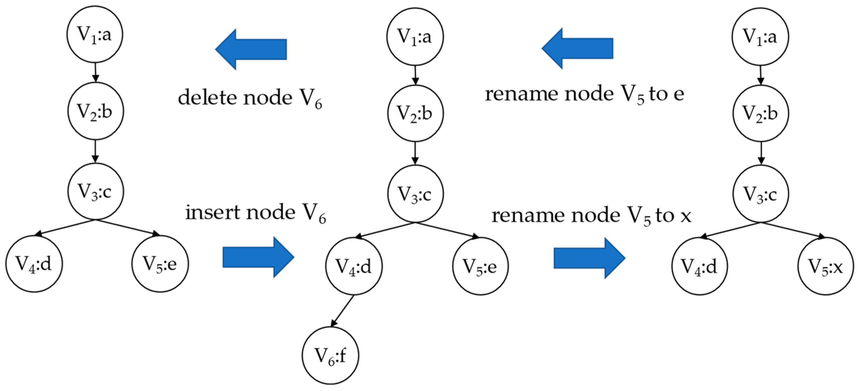
3.5. Mathematical Semantic Graph Inference

Based on the mathematical relationships between indices analyzed in Section 3.1.2, this paper defines a similarity relationship termed “isSimilarTo”. It indicates that these two index entities are similar to an extent. Through the “isSimilarTo”, the KG of remote sensing indices can incorporate more relationships and information between indices. The following outline the main principles for inferring similarity relationships based on the semantics of mathematical formulas.

Relationship analysis on a mathematical semantic graph can be thought of as a specific algorithm on a directed acyclic graph (DAG). Suppose there are two mathematical formulas A and B to be compared, represented by two DAGs: G_A = (V_A, E_A) and G_B = (V_B, E_B), respectively. Here, V_A and E_A represent the vertex and edge sets of G_A, while V_B and E_B represent those of G_B. In this process, each node (except the root node) represents an operand, and each edge represents an operator.

Because of the complexity of graph structure, computing distance with graphs has an exponential computational cost. Since the semantic graph of mathematical expressions is a special type of tree structure, it is feasible to quantify similarity using the tree edit distance (TED) algorithm, which has a lower computational cost [80].

The TED method refers to the complexity of transforming one tree into another through editing. The similarity algorithm based on tree edit distance computes the ordered distance between labeled trees, representing the minimum cost sequence of node operations required to transform one tree into another.

As shown in Figure 8, the three common editing operations defined by TED are as follows:

• Delete node: Link its child nodes to the parent node to maintain order.
• Insert a node between a known node and a contiguous subsequence of its child nodes.
• Modify the label of a node.

Each iteration of the three editing operations has a cost. The algorithm seeks the least expensive sequence of operations. Recursive methods can be used to deal with TED algorithms, but they can become exponentially complex. It is noteworthy that TED often shows significant performance variations between best- and worst-case scenarios. To increase its feasibility, Pawlik and Augsten proposed RTED, a more robust TED algorithm [81]. Because RTED ensures optimal TED performance in both best and worst-case scenarios, the RTED algorithm has been employed for semantic analysis of formulas across numerous disciplines [77,79]. Currently, the state-of-the-art algorithm in this field is AP-TED (All Path Tree Edit Distance) [82], which is widely considered an effective exact TED [83,84]. In this paper, the AP-TED algorithm is employed as the distance metric for semantic graph similarity, proposing a method for calculating the similarity of semantic graphs for remote sensing index formulas.

$$\mathsf{\gamma }=\max (1-\frac{d_{\mathit{sd}}}{{\mathrm{N}}_d},0)$$

(11)

where γ represents the similarity between the source tree (reference tree) and the target tree (comparison tree), taking a floating-point value between 0 and 1. $d_{\mathit{sd}}$ denotes the precise tree edit distance computed by the AP-TED algorithm, and ${\mathrm{N}}_d$ is the size of the target tree.

4. Construction and Application of RSIKG

Section 3 mainly introduces the modeling and knowledge representation methods for remote sensing index knowledge graphs. This section will focus on the process of constructing RSIKG and application examples.

As shown in Figure 9, the main process of constructing RSIKG is divided into the following phases:

• Ontology design and modeling: Based on a synthesis of various sources of reference materials on remote sensing indices, relevant concepts and their relationships are abstracted and modeled into ontologies. The next section introduces the tools employed and details of the process in this step.
• Data processing and database mapping: This step mainly deals with processing the index metadata and mathematical semantics of remote sensing indices, which are stored in a relational database. These data are mapped to resource description framework (RDF) files using a database mapping tool. Formula semantics are stored as attributes during this process. For more information, please refer to Section 4.2.
• Query and reasoning: This step utilizes SPARQL queries on RDF triples using Jena. Simultaneously, RDF triples are imported into Neo4J for property graph analysis and visualization of results. Additionally, the extension function of the query statement is implemented based on the semantic similarity inference method proposed in Section 3.5.

4.1. Ontology Design and Modeling

Knowledge representation methods include various approaches such as ontology, semantic networks, and frame-based models. Among them, ontology is a commonly used knowledge representation method, forming a formal system consisting of concepts, properties, and relationships to describe knowledge in a particular domain. It can be represented using standard languages such as the Web Ontology Language (OWL) and RDF.

In this phase, we introduce the role of developer, a person who manipulates the various tools needed to carry out the RSIKG process. A top-down design is demonstrated to construct the RSIKG ontology model. Ontologies in RSIKG include indices, sensors, bands, land covers, etc. Protege-5.6.2 software (https://protege.stanford.edu/, accessed on 22 August 2023) is employed by the RSIKG developer in accordance with the ontology modeling approach outlined in this study. The concepts, properties, and relationships of remote sensing indices are translated into entities, properties, and relationships (Figure 3).

As shown in Figure 10, the ontology model of the remote sensing index KG primarily encompasses indices, references, sensors, environmental resources, and band operations. In addition to the conceptual relationships illustrated in Figure 3, it also incorporates the semantic similarity discussed in Section 3.5. This involves calculating whether two index entities have a similarity relationship based on a threshold.

Table 6. Entities and their primary attributes in RSIKG.

Entity	Property	Description
Index	Name	The name representing the index, such as normalized difference vegetation index (NDVI), is utilized.
	Formula	The calculation formula representing the index, such as NDVI = (NIR − RED)/(NIR + RED).
	Coefficient	The unknown coefficients within the index are typically determined empirically or through fitting.
	Abbreviation	The abbreviated form denoting the index name, such as NDVI, EVI, etc.
Sensor	Name	The designation of the sensor, such as Landsat 8 OLI, Sentinel 2 MSI, etc.
	Resolution	The spatial resolution of the sensor imagery, such as 30 m, 10 m, etc.
Band	Name	Band names or band ID, such as RED, NIR, SWIR, corresponds to the ontology’s basic categories.
	WL_start	The starting wavelength of the electromagnetic wave corresponding to the spectral band
	WL_end	The terminating wavelength of the electromagnetic wave corresponding to the spectral band
	WL_mid	The mid-wavelength of the electromagnetic wave corresponding to the spectral band.
	SpatRes	The spatial resolution of the spectral band is indicated. The unit is in meters.
BandsMath	derivedEqu	The formula for index applied to the sensor’s band operations.
EnvRes	Name	The name of environmental resources, such as Agriculture, Forestry, Metal, Soil.
	Description	Descriptive information of environmental resources.
Reference	Title	Title of the reference literature.
	Year	Year of publication of the reference literature.
	Author	Author(s) of the reference literature.
	Journal	The journal in which the reference literature is published.
	Keywords	The keywords associated with the reference literature.

provides explanations of key attributes for each entity of the ontology.

4.2. Data Processing and Database Mapping

4.2.1. Data Collection and Processing

We introduce in this section the role of data collector and data maintainer, people who control processes and data. A raw dataset containing information on remote sensing indices, including definitions, formulas, relevant environmental resources, and references, is collected from various data sources, such as remote sensing literature, databases, and websites. These data are extracted automatically, semi-automatically, or even manually by the data collector using several extraction tools (see

Table 7. Different sources of information and their processing methods.

Information	Sources	Processing Tools and Methods
Meta-information of references (title, authors, publication, etc.)	Digital PDF files	Automatically extracted by the python library pdf2bib
Equations in references	PDF files	Automatically extracted by the method described in Section 3.4.1.
Equations, meta information from web	Website	Python web scraping libraries (Beautiful Soup, Requests)
Other information that cannot be easily automatically extracted		Data collectors manually input and correct data.

).

As shown in Table 7, for example, meta-information of references including title, authors, and publication can be extracted automatically from digital PDF files. When the source document is in LaTeX or MathML format, the mathematical formulas are directly read and saved by the formula preserved in Section 3.4.2. For PDF documents, computer vision and optical character recognition (OCR) techniques are employed to convert equations from images or PDF files to text, which is automatically saved as MathML documents. To facilitate the reading of data by multiple tools, the raw data is saved in CSV format.

The stored MathML is converted into CMML using the method shown in Figure 5. After the initial data collection, data maintainers are responsible for quality control and processing to eliminate duplicates, errors, incompleteness, or inconsistencies, thereby improving the data’s quality and usability. To ensure band name consistency, the data collector or maintainer must adopt a unified naming style of band names, aligning variations such as red, Red, R, and ${\rho }_R$ to Red. In cases where two different formulas represent the same index and annotation, comparison and verification are carried out by data maintainers to choose the correct or more common formula.

4.2.2. Data Storage and Ontology Mapping

MySQL is used to store the previously collected data and serves as the data source of RDF triples. Six tables are created in the MySQL database to correspond with the entities and relationships in Figure 10 and the entity-relationships diagram shown in Figure 11. These tables store attribute data for indices and other entities. Additionally, seven relationship tables are designed to preserve relationships between different entity tables. This lays the groundwork for data mapping.

After the data are stored in MySQL, the data can be mapped into the KG data format based on the ontology model. The transformed entities, attributes, and relationships are stored in a suitable KG database for subsequent querying and inference. Graph databases or triple-store databases are commonly used models for storing and managing KG data. For instance, indices can be stored in the following database:

• Graph database: Indices are represented as nodes, their attributes serve as node labels or properties, and their relationships are depicted as edges between nodes.
• Triple-store database: Indices function as subjects, their attributes act as predicates, and their attribute values serve as objects, forming a triple. The relationships can also be expressed as predicates, with the relationship objects as additional objects, forming another triple. This work employs the triple standard RDF for storing KG data.

To map a database to RDF, we need to convert data from a relational database into an RDF graph. This process can be achieved through direct mapping or indirect mapping. Direct mapping, which automatically maps relational database data structures to RDF triples, is rarely used in practice. Indirect mapping is a flexible and practical approach for mapping relational databases to RDF through an intermediate layer.

This paper employs the D2RQ tool for the indirect mapping of the database to RDF [16]. D2RQ is an open-source tool that provides a logical mapping layer between databases and RDF. It enables various RDF tools to access and process data in the database. Initially, a D2RQ mapping file needs to be created, defining the tables and fields in the database and how they map to classes and properties in the RDFS/OWL ontology. For instance, the mapping file can specify that the “Name” field corresponds to the “sensorName” property. Similarly, associations between different tables can be defined through each field, forming triples in the RDF. In this study, the generated RDF file contains 3,446,576 triples.

After the mapping rules are defined, the D2RQ tool can be utilized by the RSIKG developer to generate the RDF graph. The mapping file for the database should be sent to the D2RQ server when it is started. The database content is then dynamically transformed into an RDF graph by the D2RQ server, and the server sends the output back to the client. The queried data is converted into entities, properties, and relationships between entities in the KG during this process. For instance, Landsat can be represented as a sensor entity, with properties such as Name and Resolution, and relationships such as containsBands (indicating the bands it includes) and isAppliedFor (specifying the applied environmental resources).

4.3. The Query and Reasoning Phase

The process of converting index-related information from the MySQL database into RDF document format has been discussed in the previous section. Here we proceed with the process of querying and reasoning. Firstly, RDF data needs to be imported into Jena and loaded by the developer, setting up the ontology file shown in Figure 9. Then, the SPARQL reasoning service of Jena is initiated. The key steps of this phase include:

• Ontology file configuration: Jena is configured with an ontology file by the RSIKG developer in accordance with the design in Figure 10. This ensures that our KG reasoning can correctly understand and process relevant entities and relationships.
• RDF data import and loading: The raw RDF data extracted from the MySQL database is imported into the TDB graph data store of Jena. This step is the foundation for building KG reasoning.
• Query and reasoning: Jena is employed in this step. The developer launches Jena’s SPARQL reasoning service. SPARQL is a language for querying and manipulating RDF data. By using Jena’s SPARQL query and reasoning capabilities, various complex queries and reasoning operations can be performed by users on the KG. Engineering optimizations can be applied to query parsing, optimization, and execution to achieve effective graph data querying and reasoning functions, consequently improving performance.
• Result output: This step consists of presenting the results of RSIKG graph querying and reasoning to the user in an appropriate format. Users can visualize the results or export the data from the graph database.

Moreover, this system can effectively handle and analyze a large amount of index-related data, providing valuable insights and recommendations for remote sensing researchers.

4.4. Graph Visualization Analysis

The above mainly introduces a series of graph operations and analyses completed for the RDF standard format, while KGs organize data into visually intuitive graph structures, providing an intuitive representation that is easy to understand. We used the Neo4j graph database (https://neo4j.com/, accessed on 22 August 2023) for visual analysis of the graph. Neo4j is a graph database management system that efficiently stores and queries graph-structured data and is widely used for processing complex relational data.

This section explores converting RDF data into attribute graphs and importing them into the Neo4j graph database for effective graphical operations and analysis. To achieve this goal, we adopted the open-source extension package Neosemantics (n10s) from Neo4j, which directly imports RDF file formats into the Neo4j database (Code 2). After the data import is complete, the developer uses Neo4j’s query and graph visualization features to conduct exploratory analysis and presentation of the data.

Code 2. Imports RDF from an url (file or http) and stores it in Neo4j as a property graph

CALL n10s.graphconfig.init(); CREATE CONSTRAINT n10s_unique_uri for (r:Resource) require r.uri IS UNIQUE; CALL n10s.graphconfig.set({handleVocabUris: “IGNORE”}); CALL n10s.rdf.import.fetch(‘file:///tmp/rsikg_mapping_mod.nt’, ‘N-Triples’);

Through Code 2, the data can be directly imported from the RDF data defined by the ontology designed in the previous Protégé into Neo4j, avoiding the tedious process of importing individual CSV data tables as described in Literature [16], ensuring the consistency of data throughout.

As shown in Figure 12, the “ind” entity is represented by the orange-red circle, the “bandmath” entity by the deep green circle, and the “sensor” entity by the orange-yellow circle. The analysis based on attribute graphs can intuitively display the associations between different conceptual entities, which helps users extract patterns and regularities hidden in the network and convert them into meaningful information and knowledge. By using these graph analysis tools effectively, researchers can gain a better understanding of the connections between ideas, which will help them make better decisions and solve problems. Several analyses and applications based on these kinds of attribute graphs are covered in the following.

4.5. Property Graph Analysis and Applications

4.5.1. Relevant Analysis in the Field of Environmental Resources

Through the use of the remote sensing index KG, relevant analysis can be performed by users in the field of environmental resources, thus providing valuable information for a specific environmental resource study to learn indices concepts.

In the RSIKG, various indices are organized into a DAG, where indices and environmental resources are represented as nodes (Figure 13a), and edges represent their relationships. This structure can help us quickly find remote sensing indices related to specific environmental resources.

For example, if we want to study the status of soil resources in a certain area, users can use the remote sensing index KG to find remote sensing indices related to soil resources (Figure 13b). By analyzing these indices, users can learn about the distribution of soil resources, soil conditions, and water resource utilization information in the region.

In addition, the graph relationships between sensors and resources, such as soil, are significant for research. Through the analysis and mining of the graph relationships between sensors and resources such as soil established by RSIKG, it is possible to quickly understand the observation capabilities of various sensors for resources such as soil under different environmental conditions. This helps to choose the most suitable sensor in practical applications to improve the accuracy and efficiency of remote sensing monitoring.

Similar to the relationship between indices and the field of environmental resources, the environment resources and sensors in the RSIKG are also represented as nodes and edge graph relationships (Figure 14a), enabling rapid association screening in graph databases to find all known indices related to soil resources (Figure 14b).

The graph relationships can help researchers discover potential limitations of sensors when observing resources such as soil, for example: Some sensors may have poor observation effects on specific types of soil or resources. This is significant for our optimization of sensor configuration and improvement of the application level of remote sensing technology.

4.5.2. Multi Sensor Correlation Analysis

Remote sensing indices have a close relationship with multi-sensor data. Multi-sensor data provides information from different bands and sensors, which can be used to calculate various remote sensing indices, thus more comprehensively understanding the characteristics and changes of the Earth’s surface. In RSIKG, the shortest path algorithm can be used to find the shortest path between two different sensors, that is, the association relationship between these two sensors.

The Dijkstra algorithm is a very classic graph theory algorithm that can find the shortest path between two vertices in a graph. In RSIKG, each sensor can be regarded as a vertex, and the association relationship between two sensors can be regarded as an edge. Then, the shortest path algorithm can be used to find the shortest path between any two sensors. By executing the code in Code 3, Neo4j can quickly determine for users the shortest path between any two arbitrary sensors. This path represents the association relationship between these two sensors and is derived from the complex relationships between sensors and indices shown in Figure 15a.

Code 3. Analysis of the shortest path between two sensors.

MATCH (p1:sensor {sensor_Name:“GLI”}),(p2:sensor{sensor_Name:“SPOT 6”}), p=shortestpath((p1)-[*..10]-(p2)) RETURN p

As shown in Figure 15b, the shortest path between SPOT 6 and GLI can be determined by using the node ind_Name: Single Band 660. This suggests that there is a relationship between the Single Band 660 index and SPOT 6 and GLI. It is possible to use data from both sensors when calculating this index. The advantage of this approach is that it reveals the association between sensors without relying on complex mathematical models or presumptions. Large-scale sensor networks can also benefit from the shortest path algorithm’s effective application because of its comparatively low computational complexity.

4.6. The Semantic Inference of Remote Sensing Index

Based on the index semantic information and semantic graph reasoning in RSIKG, queries for remotely sensed indices with similar mathematical semantics can be performed. Setting the remotely sensed index NDVI as the reference index and using as a reference formula Equation (3), the semantic reasoning traverses all index formulas in the data and calculates their semantic similarity. According to the results of the calculation, the comparison result of the similarity degree is obtained.

As shown in

Table 8. The result of calculating index similarity based on NDVI as a reference.

Index	Formula	Distance	Similarity
NDVI	$\frac{\mathrm{NIR}-\mathrm{Red}}{\mathrm{NIR}+\mathrm{Red}}$	0	1
NDVI rededge	$\frac{\mathrm{rededge}-\mathrm{Red}}{\mathrm{rededge}+\mathrm{Red}}$	2	0.86
NBR	$\frac{\mathrm{NIR}-\mathrm{SWIR}}{\mathrm{NIR}+\mathrm{SWIR}}$	2	0.86
NDRE	$\frac{\mathrm{NIR}-\mathrm{rededge}}{\mathrm{NIR}+\mathrm{rededge}}$	2	0.86
MNDVI	$\frac{\mathrm{NIR}-\mathrm{MIR}}{\mathrm{NIR}+\mathrm{MIR}}$	2	0.86
	……
RDVI	$\frac{800 \mathrm{nm}-670 \mathrm{nm}}{ {(800 \mathrm{nm}+670 \mathrm{nm})}^{0.5}}$	9	0.53
DmSR	$\frac{\mathrm{DR}(720 \mathrm{nm})-\mathrm{DR}(500 \mathrm{nm})}{\mathrm{DR}(720 \mathrm{nm})+\mathrm{DR}(500 \mathrm{nm})}$	24	0.29
ARI	$\frac{1}{500 \mathrm{nm}}-\frac{1}{700 \mathrm{nm}}$	16	0
Ferrous iron	$\frac{[2145:2185]}{[760:860]}+\frac{[520:600]}{[630:690]}$	16	0

, based on the index similarity calculation method proposed in this paper, Equation (11), the edit distance and similarity of each index to the reference index were obtained. When the similarity is high, the distance is generally small, indicating a significant similarity between the index and the reference index in terms of both structure and operators in the formula. Specifically, NDVI is the referenced index, resulting in an edit distance of 0 and a similarity of 1. The subsequent rows of indices are derived from the NDVI formula by replacing one band in both the numerator and denominator, resulting in an edit distance of 2, representing two node renaming operations.

In cases where the target tree has a larger number of nodes and a relatively complex structure (e.g., DmSR), the edit distance value is comparatively large. This is because the edit distance does not account for the number of nodes, while the similarity formula includes the size of the target tree itself. Despite the larger numerical value, it still remains greater than 0, indicating a structurally similar relationship with the reference tree. A threshold, such as 0.5, can be set based on this similarity result to automatically infer the similarity relationships between index entities in RSIKG.

5. Discussion and Limitation

Literature reviews show us that the existing KG research in the fields of remote sensing does not focus on the specialized study of the increasingly diverse remote sensing indices. The main issues are the absence of ontology models and limited research on indices, leading to difficulties in knowledge acquisition and updates, coupled with the lack of techniques for analyzing their mathematical semantics. Starting from this point of view, for the first time in the literature, we propose a remote sensing index KG called RSIKG and its construction method, proposing a novel semantic hierarchical graph structure, consisting of an entity relationship layer for ontology modeling based on remote sensing indices, and a mathematical semantic layer for semantic expression and analysis of index formulas. In the entity relationship layer, we conducted ontology modeling of related concepts and their relationships based on the analysis and summary of the classification and common information of indices, which is more applicable for the management of index knowledge than the traditional database approach. In addition, the mathematical formula semantic information of the index formula is represented and processed in the mathematical semantic layer, which adds one more type of graph structure semantic information compared to the existing KG construction methods in geographic information or remote sensing fields. Based on the current leading semantic distance calculation method, we proposed a method for calculating the semantic similarity of remote sensing indices, greatly increasing the intelligence of the graph.

RSIKG can help users quickly grasp complex information about remote sensing indices, which could improve analysis efficiency. It can be seen that through the graph query and analysis of RSIKG, users can quickly and intuitively obtain the required information based on RSIKG. Through the calculation of the semantic similarity of the index, users can also quickly find indices similar to the reference index. However, the current semantic reasoning of index formulas is still in its early stages, and it is still difficult to automatically reason about the formula transformation and derivation process between different indices from the index formula. There is still considerable room for development in the mining of mathematical semantics.

Furthermore, the main purpose of this paper is to confirm the efficacy of the similarity calculation method that uses the tree editing distance algorithm. On the theoretical ground, more work needs to be done on the variations in editing distance brought about by each component change between various trees, taking into account the significance of remote sensing indices. The use of remote sensing index formulas may not be entirely appropriate with the current tree editing distance.

Our approach organizes entities and mathematical semantics hierarchically. It is more suitable for the practical conditions of building KGs for remote sensing indices. In fact, another possible method is to directly construct graphs through formula semantics [85]. However, for remote sensing indices, this approach is currently not feasible. First, the most important factor in the context of remote sensing indices is the relationship between indices and related concepts, which is hard to fully capture from mathematical formulas. Rather, it is more appropriate to use a combination of both approaches. Secondly, it is difficult to build such graphs primarily using remote sensing formula mathematical semantics due to the absence of contextual information related to formula semantics.

Other useful information related to index formulas, such as formula interpretation texts and symbol explanations, is added during the RSIKG construction process to help users annotate. This is due to the fact that the main workload during the construction process is extracting and processing formulas. Extensive research has been done in these areas. Nevertheless, the alignment of mathematical formulas with textual semantics remains a challenging research issue [86], and the development of context-aware semantic alignment techniques in this field is not feasible due to the lack of data sets and associated data annotation for this task. However, with the application of this approach, a better dataset can be provided for quantitative remote sensing model semantic alignment datasets. Using natural language processing (NLP) techniques, it is possible to match and align natural language descriptions found in literature with the semantics of mathematical formulas. Formulas’ semantics can be automatically linked to relevant entities and relations that are taken from natural language descriptions using named entity recognition (NER) or relation extraction (RE) techniques. These connections are then stored as nodes and edges in KG.

6. Conclusions and Future Prospects

This research introduces the concept of remote sensing indices knowledge graph (RSIKG) and its construction method, which addresses the challenges of managing and utilizing remote sensing indices. RSIKG leverages mathematical formulas and NLP techniques to extract semantic information from various remote sensing literature, providing a more efficient and less subjective approach to knowledge storage. It also explores methods to optimize the construction process, enhancing accuracy and scalability. This study aims to offer a novel KG solution for a deeper understanding and application of remote sensing data in the field of data processing and analysis. Additionally, it provides new perspectives and methods for researchers in the KG and GIS domains, bridging the gap in knowledge representation and management for remote sensing indices.

The following future directions for remote sensing index KG research are anticipated:

• Deep learning-based mathematical reasoning: Currently, mathematical semantic processing is challenging due to the complex structures of equations, which contain numerous mathematical symbols and operational rules, and their semantics usually require specific domain expertise. In recent years, the continuous development of graph embedding and graph neural networks has gained more attention from scholars [87]. It is expected that more studies about mathematical semantic processing will emerge in the future, providing stronger support for representing and analyzing mathematical knowledge to generate comprehensive indices.
• The construction of multimodal KGs: Our primary research focus aims to establish a usable index graph database based on remote sensing satellite image data. It also aims to provide analytical capabilities, intending to offer a framework for establishing relationships among satellite sensors, bands, remote sensing indices, and other information. The construction of biophysical information among indices may be a future direction for investigation. For example, building ontologies related to climate conditions such as temperature, humidity, precipitation, or variables concerning soil area and types. Additionally, exploring methods for calculating indices with multimodal ontologies to broaden their application in remote sensing indices could facilitate the exploration of new comprehensive indices.
• High-dimensional data subspace clustering: Data dimensions are increasing as a result of multimodal and multisensor information [88], particularly multispectral and hyperspectral remote sensing data, posing typical high-dimensional data challenges [89,90]. Further investigation of algorithms integrating high-dimensional data subspace clustering with RSIKG is required. This includes investigating the use of high-dimensional data subspace clustering and transfer learning algorithms [91] in various scenarios.
• Visualization and interaction of KGs: Visualization and interaction are significant components in the research of KGs. Through visualization techniques, complex remote sensing data can be transformed into easily comprehensible graphics, allowing non-professionals to comprehend the meaning of remote sensing data as well. Additionally, GraphXR, which incorporates the capabilities of augmented reality into KGs, allows for a more powerful mode of knowledge presentation [92]. In future studies, we should pay attention to the connection between KGs and AR maps [93,94]. A more intuitive visualization and interaction of KG should be developed in the future.

References

1. Gao, L.; Wang, X.; Johnson, B.A.; Tian, Q.; Wang, Y.; Verrelst, J.; Mu, X.; Gu, X. Remote Sensing Algorithms for Estimation of Fractional Vegetation Cover Using Pure Vegetation Index Values: A Review. ISPRS J. Photogramm. Remote Sens. 2020, 159, 364–377. [Google Scholar] [CrossRef] [PubMed]
2. Wu, X.; Shi, W.; Tao, F. Estimations of Forest Water Retention across China from an Observation Site-Scale to a National-Scale. Ecol. Indic. 2021, 132, 108274. [Google Scholar] [CrossRef]
3. Honarbakhsh, A.; Tahmoures, M.; Afzali, S.F.; Khajehzadeh, M.; Ali, M.S. Remote Sensing and Relief Data to Predict Soil Saturated Hydraulic Conductivity in a Calcareous Watershed, Iran. Catena 2022, 212, 106046. [Google Scholar] [CrossRef]
4. Zhang, M.; Shi, W.; Ren, Y.; Wang, Z.; Ge, Y.; Guo, X.; Mao, D.; Ma, Y. Proportional Allocation with Soil Depth Improved Mapping Soil Organic Carbon Stocks. Soil Tillage Res. 2022, 224, 105519. [Google Scholar] [CrossRef]
5. Chen, J.; Chen, S.; Fu, R.; Li, D.; Jiang, H.; Wang, C.; Peng, Y.; Jia, K.; Hicks, B.J. Remote Sensing Big Data for Water Environment Monitoring: Current Status, Challenges, and Future Prospects. Earths Future 2022, 10, e2021EF002289. [Google Scholar] [CrossRef]
6. Camps-Valls, G.; Campos-Taberner, M.; Moreno-Martínez, Á.; Walther, S.; Duveiller, G.; Cescatti, A.; Mahecha, M.D.; Muñoz-Marí, J.; García-Haro, F.J.; Guanter, L.; et al. A Unified Vegetation Index for Quantifying the Terrestrial Biosphere. Sci. Adv. 2021, 7, eabc7447. [Google Scholar] [CrossRef] [PubMed]
7. Wang, Z.; Chen, T.; Zhu, D.; Jia, K.; Plaza, A. RSEIFE: A New Remote Sensing Ecological Index for Simulating the Land Surface Eco-Environment. J. Environ. Manag. 2023, 326, 116851. [Google Scholar] [CrossRef]
8. Vayssade, J.-A.; Paoli, J.-N.; Gée, C.; Jones, G. DeepIndices: Remote Sensing Indices Based on Approximation of Functions through Deep-Learning, Application to Uncalibrated Vegetation Images. Remote Sens. 2021, 13, 2261. [Google Scholar] [CrossRef]
9. Chen, H.; Li, H.; Liu, Z.; Zhang, C.; Zhang, S.; Atkinson, P.M. A Novel Greenness and Water Content Composite Index (GWCCI) for Soybean Mapping from Single Remotely Sensed Multispectral Images. Remote Sens. Environ. 2023, 295, 113679. [Google Scholar] [CrossRef]
10. Barton, C.M.; Alberti, M.; Ames, D.; Atkinson, J.-A.; Bales, J.; Burke, E.; Chen, M.; Diallo, S.Y.; Earn, D.J.D.; Fath, B.; et al. Call for Transparency of COVID-19 Models. Science 2020, 368, 482–483. [Google Scholar] [CrossRef]
11. Montero, D.; Aybar, C.; Mahecha, M.D.; Martinuzzi, F.; Söchting, M.; Wieneke, S. A Standardized Catalogue of Spectral Indices to Advance the Use of Remote Sensing in Earth System Research. Sci. Data 2023, 10, 197. [Google Scholar] [CrossRef] [PubMed]
12. Gao, S.; Zhong, R.; Yan, K.; Ma, X.; Chen, X.; Pu, J.; Gao, S.; Qi, J.; Yin, G.; Myneni, R.B. Evaluating the Saturation Effect of Vegetation Indices in Forests Using 3D Radiative Transfer Simulations and Satellite Observations. Remote Sens. Environ. 2023, 295, 113665. [Google Scholar] [CrossRef]
13. Zhou, D.; Zhang, L.; Hao, L.; Sun, G.; Xiao, J.; Li, X. Large Discrepancies among Remote Sensing Indices for Characterizing Vegetation Growth Dynamics in Nepal. Agric. For. Meteorol. 2023, 339, 109546. [Google Scholar] [CrossRef]
14. Wang, H.; Fu, T.; Du, Y.; Gao, W.; Huang, K.; Liu, Z.; Chandak, P.; Liu, S.; Van Katwyk, P.; Deac, A.; et al. Scientific Discovery in the Age of Artificial Intelligence. Nature 2023, 620, 47–60. [Google Scholar] [CrossRef] [PubMed]
15. Peng, C.; Xia, F.; Naseriparsa, M.; Osborne, F. Knowledge Graphs: Opportunities and Challenges. Artif. Intell. Rev. 2023, 56, 13071–13102. [Google Scholar] [CrossRef] [PubMed]
16. Hao, X.; Ji, Z.; Li, X.; Yin, L.; Liu, L.; Sun, M.; Liu, Q.; Yang, R. Construction and Application of a Knowledge Graph. Remote Sens. 2021, 13, 2511. [Google Scholar] [CrossRef]
17. Abburu, S.; Dube, N. Ontology Concept-Based Management and Semantic Retrieval of Satellite Data. J. Intell. Syst. 2017, 26, 197–213. [Google Scholar] [CrossRef]
18. Li, Y.; Kong, D.; Zhang, Y.; Tan, Y.; Chen, L. Robust Deep Alignment Network with Remote Sensing Knowledge Graph for Zero-Shot and Generalized Zero-Shot Remote Sensing Image Scene Classification. ISPRS J. Photogramm. Remote Sens. 2021, 179, 145–158. [Google Scholar] [CrossRef]
19. Li, Y.; Ouyang, S.; Zhang, Y. Combining Deep Learning and Ontology Reasoning for Remote Sensing Image Semantic Segmentation. Knowl.-Based Syst. 2022, 243, 108469. [Google Scholar] [CrossRef]
20. Zhang, Y.; Wang, F.; Li, Y.; OuYang, S.; Wei, D.; Liu, X.; Kong, D.; Chen, R.; Zhang, B. Remote Sensing Knowledge Graph Construction and Its Application in Typical Scenarios. Natl. Remote Sens. Bull. 2023, 27, 249–266. [Google Scholar] [CrossRef]
21. Zhao, L.; Li, Q.; Chang, Q.; Shang, J.; Du, X.; Liu, J.; Dong, T. In-Season Crop Type Identification Using Optimal Feature Knowledge Graph. ISPRS J. Photogramm. Remote Sens. 2022, 194, 250–266. [Google Scholar] [CrossRef]
22. Ge, X.; Yang, Y.; Chen, J.; Li, W.; Huang, Z.; Zhang, W.; Peng, L. Disaster Prediction Knowledge Graph Based on Multi-Source Spatio-Temporal Information. Remote Sens. 2022, 14, 1214. [Google Scholar] [CrossRef]
23. Liu, X.; Zhang, Y.; Zou, H.; Wang, F.; Cheng, X.; Wu, W.; Liu, X.; Li, Y. Multi-Source Knowledge Graph Reasoning for Ocean Oil Spill Detection from Satellite SAR Images. Int. J. Appl. Earth Obs. Geoinf. 2023, 116, 103153. [Google Scholar] [CrossRef]
24. Indices Gallery—ArcGIS Pro. Documentation. Available online: https://pro.arcgis.com/en/pro-app/latest/help/data/imagery/indices-gallery.htm (accessed on 19 August 2023).
25. Alphabetical List of Spectral Indices. Available online: https://www.nv5geospatialsoftware.com/docs/alphabeticallistspectralindices.html (accessed on 22 August 2023).
26. Gorelick, N.; Hancher, M.; Dixon, M.; Ilyushchenko, S.; Thau, D.; Moore, R. Google Earth Engine: Planetary-Scale Geospatial Analysis for Everyone. Remote Sens. Environ. 2017, 202, 18–27. [Google Scholar] [CrossRef]
27. Rivera, J.; Verrelst, J.; Delegido, J.; Veroustraete, F.; Moreno, J. On the Semi-Automatic Retrieval of Biophysical Parameters Based on Spectral Index Optimization. Remote Sens. 2014, 6, 4927–4951. [Google Scholar] [CrossRef]
28. Maxant, J.; Braun, R.; Caspard, M.; Clandillon, S. ExtractEO, a Pipeline for Disaster Extent Mapping in the Context of Emergency Management. Remote Sens. 2022, 14, 5253. [Google Scholar] [CrossRef]
29. Anderson, R. Rander38/Remote-Sensing-Indices-Derivation-Tool. Available online: https://github.com/rander38/Remote-Sensing-Indices-Derivation-Tool (accessed on 23 August 2023).
30. Henrich, V.; Götze, C.; Jung, A.; Sandow, C.; Thürkow, D.; Gläßer, C. Development of an Online Indices Database: Motivation, Concept and Implementation. In Proceedings of the 6th EARSeL Imaging Spectroscopy SIG Workshop Innovative Tool for Scientific and Commercial Environment Applications, Tel Aviv, Israel, 16–18 March 2009; pp. 16–18. [Google Scholar]
31. Velastegui-Montoya, A.; Montalván-Burbano, N.; Carrión-Mero, P.; Rivera-Torres, H.; Sadeck, L.; Adami, M. Google Earth Engine: A Global Analysis and Future Trends. Remote Sens. 2023, 15, 3675. [Google Scholar] [CrossRef]
32. Tamiminia, H.; Salehi, B.; Mahdianpari, M.; Quackenbush, L.; Adeli, S.; Brisco, B. Google Earth Engine for Geo-Big Data Applications: A Meta-Analysis and Systematic Review. ISPRS J. Photogramm. Remote Sens. 2020, 164, 152–170. [Google Scholar] [CrossRef]
33. Delegido, J.; Verrelst, J.; Rivera, J.P.; Ruiz-Verdú, A.; Moreno, J. Brown and Green LAI Mapping through Spectral Indices. Int. J. Appl. Earth Obs. Geoinf. 2015, 35, 350–358. [Google Scholar] [CrossRef]
34. IDB—Index DataBase. Available online: https://www.indexdatabase.de/ (accessed on 6 August 2023).
35. Gun, Z.; Chen, J. Novel Knowledge Graph- and Knowledge Reasoning-Based Classification Prototype for OBIA Using High Resolution Remote Sensing Imagery. Remote Sens. 2023, 15, 321. [Google Scholar] [CrossRef]
36. Stewart, I. Mathematics, Maps, and Models. In The Map and the Territory: Exploring the Foundations of Science, Thought and Reality; Wuppuluri, S., Doria, F.A., Eds.; The Frontiers Collection; Springer International Publishing: Cham, Switzerland, 2018; pp. 345–356. ISBN 978-3-319-72478-2. [Google Scholar]
37. Bian, S.-F.; Li, H.-P. Mathematical Analysis in Cartography by Means of Computer Algebra System. In Cartography—A Tool for Spatial Analysis; Bateira, C., Ed.; InTech: Rijeka, Croatia, 2012; ISBN 978-953-51-0689-0. [Google Scholar]
38. Subrt, T.; Brozova, H. Knowledge Maps and Mathematical Modelling. Electron. J. Knowl. Manag. 2007, 5, 497–504. [Google Scholar]
39. Shen, F. A United Framework for Both Formal, Natural and Social Science 2022. arXiv 2022, arXiv:2105.04036. [Google Scholar] [CrossRef]
40. Brožová, H.; Šubrt, T.; Bartoška, J. Knowledge Maps in Agriculture and Rural Development. Agric. Econ. Zemědělská Ekon. 2008, 54, 546–552. [Google Scholar] [CrossRef]
41. Fionda, V.; Gutierrez, C.; Pirrò, G. Building Knowledge Maps of Web Graphs. Artif. Intell. 2016, 239, 143–167. [Google Scholar] [CrossRef]
42. Moradi, F. Effectiveness of Concept Mapping’s Efficiency in Differential Equations. Inf. Investig. Ens. Inéd. 2020, 20, 1–23. [Google Scholar] [CrossRef]
43. Maraee, A.; Sturm, A. Formal Semantics and Analysis Tasks for ME-MAP Models. In Proceedings of the 2017 11th International Conference on Research Challenges in Information Science (RCIS), Brighton, UK, 10–12 May 2017; pp. 234–243. [Google Scholar]
44. Elizarov, A.; Kirillovich, A.; Lipachev, E.; Nevzorova, O.; Solovyev, V.; Zhiltsov, N. Mathematical Knowledge Representation: Semantic Models and Formalisms 2014. arXiv 2014, arXiv:1408.6806. [Google Scholar] [CrossRef]
45. Pardos, Z.A.; Nam, A.J.H. A Map of Knowledge 2018. arXiv 2018, arXiv:1811.07974. [Google Scholar] [CrossRef]
46. Wang, C.; Yue, T.; Fan, Z. Semantic Analysis and Mapping of Resource and Environmental Mathematical Models. Comput. Eng. Appl. 2013, 49, 1–6. [Google Scholar] [CrossRef]
47. Wang, C.; Yue, T.; Fan, Z. Formal Linguistic Research of Resource and Environment Model Compound Based on Model-Flow. J. Geo-Inf. Sci. 2014, 16, 31–38. [Google Scholar] [CrossRef]
48. Lu, Y.; Yue, T.; Wang, C.; Wang, Q. Workflow-Based Spatial Modeling Environment and Its Application in Food Provisioning Services of Grassland Ecosystem. In Proceedings of the 2010 18th International Conference on Geoinformatics, Geoinformatics 2010, Beijing, China, 18–20 June 2010; IEEE Computer Society: Washington, DC, USA, 2010; pp. 1–6. [Google Scholar]
49. Wang, C.; Yue, T. A Software Tool for Earth Surface Modeling of Environmental Variables. Procedia Environ. Sci. 2012, 13, 565–573. [Google Scholar] [CrossRef]
50. Xue, J.; Su, B. Significant Remote Sensing Vegetation Indices: A Review of Developments and Applications. J. Sens. 2017, 2017, 1353691. [Google Scholar] [CrossRef]
51. Rouse, J.W.; Haas, R.H.; Schell, J.A.; Deering, D.W. Monitoring Vegetation Systems in the Great Plains with ERTS. Nasa Spec. Publ. 1974, 351, 309–317. [Google Scholar]
52. Bannari, A.; Morin, D.; Bonn, F.; Huete, A.R. A Review of Vegetation Indices. Remote Sens. Rev. 1995, 13, 95–120. [Google Scholar] [CrossRef]
53. Gao, B. NDWI—A Normalized Difference Water Index for Remote Sensing of Vegetation Liquid Water from Space. Remote Sens. Environ. 1996, 58, 257–266. [Google Scholar] [CrossRef]
54. Zha, Y.; Gao, J.; Ni, S. Use of Normalized Difference Built-up Index in Automatically Mapping Urban Areas from TM Imagery. Int. J. Remote Sens. 2003, 24, 583–594. [Google Scholar] [CrossRef]
55. Bhatti, S.S.; Tripathi, N.K. Built-up Area Extraction Using Landsat 8 OLI Imagery. GIScience Remote Sens. 2014, 51, 445–467. [Google Scholar] [CrossRef]
56. Hall, D.K.; Riggs, G.A.; Salomonson, V.V. Development of Methods for Mapping Global Snow Cover Using Moderate Resolution Imaging Spectroradiometer Data. Remote Sens. Environ. 1995, 54, 127–140. [Google Scholar] [CrossRef]
57. Hall, D.K.; Riggs, G.A. Normalized-Difference Snow Index (NDSI). In Encyclopedia of Snow, Ice and Glaciers; Singh, V.P., Singh, P., Haritashya, U.K., Eds.; Springer: Dordrecht, The Netherlands, 2011; pp. 779–780. ISBN 978-90-481-2642-2. [Google Scholar]
58. Hall, D.K.; Riggs, G.A.; Salomonson, V.V.; DiGirolamo, N.E.; Bayr, K.J. MODIS Snow-Cover Products. Remote Sens. Environ. 2002, 83, 181–194. [Google Scholar] [CrossRef]
59. Meyer, L.H.; Heurich, M.; Beudert, B.; Premier, J.; Pflugmacher, D. Comparison of Landsat-8 and Sentinel-2 Data for Estimation of Leaf Area Index in Temperate Forests. Remote Sens. 2019, 11, 1160. [Google Scholar] [CrossRef]
60. Li, P.; Jiang, L.; Feng, Z. Cross-Comparison of Vegetation Indices Derived from Landsat-7 Enhanced Thematic Mapper Plus (ETM+) and Landsat-8 Operational Land Imager (OLI) Sensors. Remote Sens. 2013, 6, 310–329. [Google Scholar] [CrossRef]
61. Widlowski, J.-L.; Verstraete, M.M.; Pinty, B.; Gobron, N. Advanced Vegetation Indices Optimized for Up-Coming Sensors: Design, Performance, and Applications. IEEE Trans. Geosci. Remote Sens. 2000, 38, 2489–2505. [Google Scholar] [CrossRef]
62. Zeng, Y.; Hao, D.; Huete, A.; Dechant, B.; Berry, J.; Chen, J.M.; Joiner, J.; Frankenberg, C.; Bond-Lamberty, B.; Ryu, Y.; et al. Optical Vegetation Indices for Monitoring Terrestrial Ecosystems Globally. Nat. Rev. Earth Environ. 2022, 3, 477–493. [Google Scholar] [CrossRef]
63. Jordan, C.F. Derivation of Leaf-Area Index from Quality of Light on the Forest Floor. Ecology 1969, 50, 663–666. [Google Scholar] [CrossRef]
64. Richardson, A.J.; Wiegand, C. Distinguishing Vegetation from Soil Background Information. Photogramm. Eng. Remote Sens. 1977, 43, 1541–1552. [Google Scholar]
65. Badgley, G.; Field, C.B.; Berry, J.A. Canopy Near-Infrared Reflectance and Terrestrial Photosynthesis. Sci. Adv. 2017, 3, e1602244. [Google Scholar] [CrossRef] [PubMed]
66. Baldocchi, D.D.; Ryu, Y.; Dechant, B.; Eichelmann, E.; Hemes, K.; Ma, S.; Sanchez, C.R.; Shortt, R.; Szutu, D.; Valach, A.; et al. Outgoing Near-Infrared Radiation from Vegetation Scales With Canopy Photosynthesis Across a Spectrum of Function, Structure, Physiological Capacity, and Weather. J. Geophys. Res. Biogeosci. 2020, 125, e2019JG005534. [Google Scholar] [CrossRef]
67. Tamašauskaitė, G.; Groth, P. Defining a Knowledge Graph Development Process Through a Systematic Review. ACM Trans. Softw. Eng. Methodol. 2023, 32, 1–40. [Google Scholar] [CrossRef]
68. IBEM. Mathematical Formula Detection Dataset. Available online: https://zenodo.org/records/4757865 (accessed on 7 September 2023).
69. breezedeus CnMFD_Dataset. Available online: https://www.kaggle.com/datasets/breezedeus/cnmfd-dataset (accessed on 7 September 2023).
70. Schmitt-Koopmann, F.M.; Huang, E.M.; Hutter, H.-P.; Stadelmann, T.; Darvishy, A. FormulaNet: A Benchmark Dataset for Mathematical Formula Detection. IEEE Access 2022, 10, 91588–91596. [Google Scholar] [CrossRef]
71. Yan, Z.; Zhang, X.; Gao, L.; Yuan, K.; Tang, Z. ConvMath: A Convolutional Sequence Network for Mathematical Expression Recognition. In Proceedings of the 2020 25th International Conference on Pattern Recognition (ICPR), Milan, Italy, 10–15 January 2021; pp. 4566–4572. [Google Scholar]
72. Deng, Y.; Kanervisto, A.; Ling, J.; Rush, A.M. Image-to-Markup Generation with Coarse-to-Fine Attention. In Proceedings of the 34th International Conference on Machine Learning, Sydney, Australia, 6–11 August 2017; Microtome Publishing: Brookline, NY, USA, 2017; Volume 70, pp. 980–989. [Google Scholar]
73. Lukas-Blecher/LaTeX-OCR: Pix2tex: Using a ViT to Convert Images of Equations into LaTeX Code. Available online: https://github.com/lukas-blecher/LaTeX-OCR (accessed on 7 September 2023).
74. Duregård, J.; Jansson, P. Embedded Parser Generators. ACM SIGPLAN Not. 2012, 46, 107–117. [Google Scholar] [CrossRef]
75. Forsberg, M.; Ranta, A. Labelled BNF: A High-Level Formalism for Defining Well-Behaved Programming Languages. Proc. Est. Acad. Sci. Phys. Math. 2003, 52, 356. [Google Scholar] [CrossRef]
76. Watabe, T.; Miyazaki, Y. Framework of a System for Extracting Mathematical Concepts from Content MathML-Based Mathematical Expressions. In Intelligent Interactive Multimedia: Systems and Services; Watanabe, T., Watada, J., Takahashi, N., Howlett, R.J., Jain, L.C., Eds.; Smart Innovation, Systems and Technologies; Springer: Berlin/Heidelberg, Germany, 2012; Volume 14, pp. 269–278. ISBN 978-3-642-29933-9. [Google Scholar]
77. Greiner-Petter, A.; Schubotz, M.; Cohl, H.S.; Gipp, B. MathTools: An Open API for Convenient MathML Handling. In Intelligent Computer Mathematics; Rabe, F., Farmer, W.M., Passmore, G.O., Youssef, A., Eds.; Lecture Notes in Computer Science; Springer International Publishing: Cham, Switzerland, 2018; Volume 11006, pp. 104–110. ISBN 978-3-319-96811-7. [Google Scholar]
78. Hussain, S.; Bai, S.; Khoja, S. Content MathML (CMML) Conversion Using LATEX Math Grammar (LMG). In Proceedings of the 2019 7th International Conference on Smart Computing & Communications (ICSCC), Sarawak, Malaysia, 28–30 June 2019; IEEE: Manhattan, NY, USA, 2019; pp. 1–5. [Google Scholar]
79. Schubotz, M.; Meuschke, N.; Hepp, T.; Cohl, H.S.; Gipp, B. VMEXT: A Visualization Tool for Mathematical Expression Trees. In Intelligent Computer Mathematics; Geuvers, H., England, M., Hasan, O., Rabe, F., Teschke, O., Eds.; Lecture Notes in Computer Science; Springer International Publishing: Cham, Switzerland, 2017; Volume 10383, pp. 340–355. ISBN 978-3-319-62074-9. [Google Scholar]
80. Dwivedi, S.P.; Srivastava, V.; Gupta, U. Graph Similarity Using Tree Edit Distance. In Proceedings of the Structural, Syntactic, and Statistical Pattern Recognition, Montreal, QC, Canada, 26–27 August 2022; Krzyzak, A., Suen, C.Y., Torsello, A., Nobile, N., Eds.; Springer International Publishing: Cham, Switzerland, 2022; pp. 233–241. [Google Scholar]
81. Pawlik, M.; Augsten, N. RTED: A Robust Algorithm for the Tree Edit Distance. Proc. VLDB Endow. 2011, 5, 334–345. [Google Scholar] [CrossRef]
82. Pawlik, M.; Augsten, N. Tree Edit Distance: Robust and Memory-Efficient. Inf. Syst. 2016, 56, 157–173. [Google Scholar] [CrossRef]
83. Pawlik, M.; Augsten, N. Minimal Edit-Based Diffs for Large Trees. In Proceedings of the 29th ACM International Conference on Information & Knowledge Management, Virtual Event, 19–23 October 2020; pp. 1225–1234. [Google Scholar]
84. Karpov, N.; Zhang, Q. SyncSignature: A Simple, Efficient, Parallelizable Framework for Tree Similarity Joins. Proc. VLDB Endow. 2022, 16, 330–342. [Google Scholar] [CrossRef]
85. Guo, Z.; Liu, Y. Research on Mathematical Formula Knowledge Base for Formula Recognition. In Proceedings of the 2018 IEEE/WIC/ACM International Conference on Web Intelligence (WI), Santiago, Chile, 3–6 December 2018; IEEE: Manhattan, NY, USA, 2018; pp. 619–622. [Google Scholar]
86. Ferreira, D.; Thayaparan, M.; Valentino, M.; Rozanova, J.; Freitas, A. To Be or Not to Be an Integer? Encoding Variables for Mathematical Text. In Proceedings of the Findings of the Association for Computational Linguistics: ACL 2022, Dublin, Ireland, 22–27 May 2022; Association for Computational Linguistics: Kerrville, TX, USA, 2022; pp. 938–948. [Google Scholar]
87. Wang, M.; Tang, Y.; Wang, J.; Deng, J. Premise Selection for Theorem Proving by Deep Graph Embedding. In Proceedings of the 31st International Conference on Neural Information Processing Systems, Long Beach, CA, USA, 4–9 December 2017; Curran Associates Inc.: Red Hook, NY, USA, 2017; pp. 2783–2793. [Google Scholar]
88. Araújo, A.F.R.; Antonino, V.O.; Ponce-Guevara, K.L. Self-Organizing Subspace Clustering for High-Dimensional and Multi-View Data. Neural Netw. 2020, 130, 253–268. [Google Scholar] [CrossRef] [PubMed]
89. Wan, Y.; Zhong, Y.; Ma, A.; Zhang, L. Multi-Objective Sparse Subspace Clustering for Hyperspectral Imagery. IEEE Trans. Geosci. Remote Sens. 2020, 58, 2290–2307. [Google Scholar] [CrossRef]
90. Cai, Y.; Zhang, Z.; Cai, Z.; Liu, X.; Jiang, X.; Yan, Q. Graph Convolutional Subspace Clustering: A Robust Subspace Clustering Framework for Hyperspectral Image. IEEE Trans. Geosci. Remote Sens. 2021, 59, 4191–4202. [Google Scholar] [CrossRef]
91. Liu, C.; Zhao, Q.; Yan, B.; Elsayed, S.; Sarker, R. Transfer Learning-Assisted Multi-Objective Evolutionary Clustering Framework with Decomposition for High-Dimensional Data. Inf. Sci. 2019, 505, 440–456. [Google Scholar] [CrossRef]
92. Sun, H.; Song, Z.; Chen, Q.; Wang, M.; Tang, F.; Dou, L.; Zou, Q.; Yang, F. MMiKG: A Knowledge Graph-Based Platform for Path Mining of Microbiota–Mental Diseases Interactions. Brief. Bioinform. 2023, 24, bbad340. [Google Scholar] [CrossRef]
93. Huang, K.; Wang, C.; Shi, W. Accurate and Robust Rotation-Invariant Estimation for High-Precision Outdoor AR Geo-Registration. Remote Sens. 2023, 15, 3709. [Google Scholar] [CrossRef]
94. Wang, C.; Huang, K.; Shi, W. An Accurate and Efficient Quaternion-Based Visualization Approach to 2D/3D Vector Data for the Mobile Augmented Reality Map. ISPRS Int. J. Geo-Inf. 2022, 11, 383. [Google Scholar] [CrossRef]
Figure 1. The framework of RSIKG based on semantic hierarchical graph.
Remotesensing 16 00158 g001
Figure 2. Node and subgraph relations of semantic hierarchical graph.
Remotesensing 16 00158 g002
Figure 3. The relationship between concepts related to remote sensing indices.
Remotesensing 16 00158 g003
Figure 4. The entire process of extracting mathematical formulas for remote sensing indices.
Remotesensing 16 00158 g004
Figure 5. The conversion of formulas representation from PMML to CMML.
Remotesensing 16 00158 g005
Figure 6. Abstract syntax tree of the NDWI equation.
Remotesensing 16 00158 g006
Figure 7. Semantic graph of the NDWI equation.
Remotesensing 16 00158 g007
Figure 8. Three common tree editing operations.
Remotesensing 16 00158 g008
Figure 9. The main construction process of RSIKG.
Remotesensing 16 00158 g009
Figure 10. Visual display of ontology structure.
Remotesensing 16 00158 g010
Figure 11. ER Diagram of the remote sensing index-related data stored in the database.
Remotesensing 16 00158 g011
Figure 12. Entities and relationships imported into Neo4j graph database: (a) a portion of imported RSIKG entities, (b) a portion of imported RSIKG relationships.
Remotesensing 16 00158 g012
Figure 13. Extraction of remote sensing indices for soil resource calculation: (a) the relationship between sensor and resource environment, (b) remote sensing indices for soil resource calculation.
Remotesensing 16 00158 g013
Figure 14. Sensors related to soil retrieved from relationship between sensor and resource Environment: (a) the relationship between sensor and resource environment (limit 100 records), (b) sensors related to soil retrieved.
Remotesensing 16 00158 g014
Figure 15. Analyzing the correlation of different modal sensors: (a) the relationship between sensor and index (limit 100 records), (b) the association path between SPOT 6 and GLI sensors.
Remotesensing 16 00158 g015