Abstract
Seismic impedance inversion is a vital way of geological interpretation and reservoir investigation from a geophysical perspective. However, it is inevitably an ill-posed problem due to the noise or the band-limited characteristic of seismic data. Artificial neural network have been used to solve nonlinear inverse problems in recent years. This research obtained an acoustic impedance profile by feeding seismic profile and background impedance into a well-trained self-attention U-Net. The U-Net got convergence by appropriate iteration, and the output predicted the impedance profiles in the test. To value the quality of predicted profiles from different perspectives, e.g., correlation, regression, and similarity, we used four kinds of indexes. At the same time, our results were predicted by conventional methods (e.g., deconvolution with recursive inversion, and TV regularization) and a 1D neural network was calculated in contrast. Self-attention U-Net showed to be robust to noise and does not require prior knowledge. Furthermore, spatial continuity is also better than deconvolution, regularization, and 1D deep learning methods in contrast. The U-Net in this paper is a type of full convolutional neural network, so there are no limits to the shape of the input. Based on this, a large impedance profile can be predicted by U-Net, which is trained by a patchy training dataset. In addition, this paper applied the proposed method to the field data obtained by the Ceduna survey without any label. The predictions prove that this well-trained network could be generalized from synthetic data to field data.
1. Introduction
Seismic inversion is a process used to translate raw survey records to rock properties, i.e., invert from the seismic data domain to the geological model domain. Generalized seismic inversion means impedance inversion. Seismic impedance is defined as a product of density with wave velocity in a subsurface medium. Concretely, it stands for vibration resistance, i.e., the wave hardly propagates in a medium with high impedance. The big differences in impedance between two neighboring mediums mean that the wave is prone to reflect at their interface, i.e., the transmission component is significantly less than the reflection. For elastic seismic waves, including P-wave and S-wave, there is the elastic impedance (EI), in which the directions of the vibration are taken into consideration. If Poisson’s ratio is known, the S-wave speed can be calculated by the P-wave speed. Based on this, acoustic impedance (AI) calculated by the speed of the P-wave is more commonly used in simplified cases.
Seismic impedance inversion is an essential component of the geological interpretation and reservoir investigation process. However, it is inevitably an ill-posed problem due to the noise or the band-limited characteristic of seismic data, and the solution is not unique [,].
From the perspective of convolution, deconvolution had an early debut and is basic in convention. The reflection coefficient at an interface is defined by the upward and downward impedance values wave-reflecting ability. In an ideal subsurface model, it is a sparse and spike sequence with time or depth. The seismic imaging profile is obtained by convoluting the R sequence with a wavelet in a survey based on the seismic convolutional theory []. Deconvolution aims to find an inverse wavelet, i.e., an inverse filter, to take out the effect of the seismic wavelet and obtain an R sequence. The impedance is computed by the recursive integration. The recursion scheme is sensitive to inaccuracy resulting from deconvolution and noises included in seismic data. The regularization is also a data-driven 2D iterative and optimized inversion method, which is effective for solving the ill-posed inversion problem. Tikhonov regularization and total variation (TV) regularization are commonly used in seismic inversion [].
Deconvolution and regularization are both based on seismic imaging profiles []. There is still a series of processing workflows between waveform records and profiles. Full waveform inversion (FWI) set up by wave equation intends to reconstruct high-resolution spatial models from the full wavefields, which include various multiple reflected waves []. A realistic subsurface model could be estimated by continually modifying the initial parameters and minimizing the difference between the actual and synthetic wavefields.
Many neural network methods have been developed for seismic data processing and interpretation [,,,,,,,,,,,,,,,]. For impedance inversion, a recurrent neural network (RNN) is widely used in 1D inversion, especially for well-log constraint cases. Das et al. [] proposed an effective 1D convolutional neural network (CNN) with two layers for the implementation of the synthetic and field data set. Mustafa et al. [] built a network by 1D CNN and achieved good results on Marmousi. Wang et al. [] applied 1D U-Net on seismic inversion to get rid of the high demand for labels.
Yet, there are many issues that need to be further investigated in their workflows. For example, some prior knowledge (e.g., type, phase and frequency of wavelet, relatively accurate background impedance profile) is needed for deconvolution and regularization [,]. For 1D methods, spatial discontinuity is prone to downgrading the predicted results. Especially for conventional methods, they are not as robust in noisy cases as neural network methods and are more sensitive to hypo-parameters. In fact, many neural networks with full connection layers are hardly useful in field cases since the shape of the input is fixed. They cannot directly output a large seismic impedance profile after processing.
This research proposed that the self-attention U-Net is applied to do seismic impedance inversion from seismic profile and background impedance. A convolutional neural network (CNN) has strong noise resistance, and U-Net based on CNN is robust and useful in seismic data processing and interpretation. Self-attention improved the final results by the correlation feature []. In this paper, the self-attention U-Net is full of convolutional layers, so there are no limits to the shape of the input data. It is possible to predict global and large impedance profiles after being trained by local profiles.
It is important for data-driven and supervised deep learning to be fed by a sufficient and polished label dataset. An image pyramid is used to augment the label data in this paper. The changing factors in field surveys are also taken into consideration to simulate reasonable cases. The input dataset with noise can be generated by a label dataset by applying a seismic convolutional model.
The network was well trained and achieved convergence by appropriate iteration, and the output predicted the impedance profiles in the test. We used four kinds of indexes to value the quality of the predicted profiles from different perspectives, e.g., correlation, regression, and similarity. At the same time, we made comparisons between the results predicted by conventional methods (e.g., deconvolution with recursive inversion, and TV regularization) and the 1D neural network.
2. Materials and Methods
2.1. Theory
2.1.1. Seismic Convolution Model
Seismic migration is a bridge from seismic records to impedance inversion. Derived from the Zoeppritz equation [] of a plane wave incident upon the horizontal interfaces, the reflection coefficient sequence can be calculated from the wave impedance sequence as (1):
where R is the reflection coefficient, Z denotes impedance, and i = 1, 2, 3, … is the layer index from the surface to the underground.
Seismic imaging profiles (i.e., pseudo seismic profiles) could be considered as reflection coefficient profiles blurred by Hessian tensor, as (2). Hessian tensor, as (3), would be influenced by the undersurface terrain and acquisition system, to an extent.
where is the seismic migration profile, is a Hessian tensor, and J is the target function based on least squares in inversion.
So, seismic impedance inversion is a problem of non-linear optimization as (5):
where f means two ordered functions, deconvolution and integration, as a nonlinear transformation operator. A Hessian operator in 2D cases is a 4D tensor, and calculating its inverse directly is costly in terms of memory and time. The DL method proposed in this paper will implement end-to-end nonlinear mapping from profile to profile, i.e., f.
2.1.2. Image Pyramid
The image pyramid as shown in Figure 1 originates from digital image processing and includes multiple-resolution images by up and downsampling from the same original image. It is helpful to detect the local or global features of an image. A Laplacian pyramid increases the resolution (i.e., upsampling), and a Gaussian pyramid decreases one (i.e., downsampling). In this paper, the image pyramid aims to augment the impedance dataset.
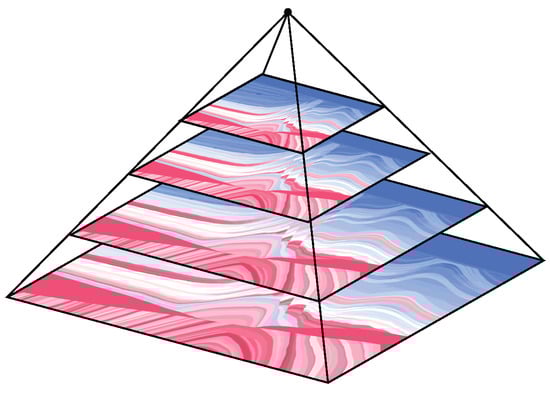
Figure 1.
Image pyramid. From up to down, the resolution is lower than the next layer.
This paper utilized three available synthetic impedance models with consistent density. To overcome the problem of insufficient data, the models with different resolutions could be sampled by the image pyramid, which is a window with a fixed shape of the models that is used to reduce the many impedance profiles. These profiles were gathered in the labeled dataset.
2.1.3. Neural Network
The neural network method is one type of iterative method and is based on backpropagation. By forwarding the calculation and gradient backpropagation, each parameter of a neuron is updated to decrease the loss value and give a fitting solution of inversion.
The self-attention U-Net is shown in Figure 2 which consists of an encoder, a decoder, and the corresponding shortcuts. The classic 2D U-Net [] is used in this paper. There are four convolutional layers with ReLU for encoders, where the kernel size is and channel size is , and means the layer depth of the encoder. The decoder has a symmetrical structure, so convolutional layers are replaced by the transposed convolutional ones.
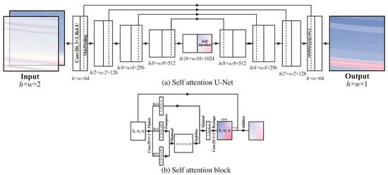
Figure 2.
Neural network architecture, (a) self-attention U-Net, (b) self-attention block. The input data with two channels (first for seismic imaging profile, second for background impedance profile) will be convoluted by four layers. Each layer has double kernels, the following activation function ReLU, and a max-pooling operation. The height and width would be cut in half, but the number of channels would be double after being convoluted by each layer. Before transpose convolution, the data is processed by a self-attention block, which is shown in (b). It gave a weighted metric to the feature map. To recover features from the high-dimension maps, there are four corresponding transposed convolutional layers. Each layer has a shortcut to concatenate features with different receptive fields. After that, the shape of the output would be the same as the input.
Different from the classic U-Net, there is a self-attention block added before the transposed convolution to be the center layer. As shown in Figure 2b, the self-attention block calculates the correlation for the feature maps of one layer output, which could provide a weight matrix and avoid the gradient of target feature vanishing. Additionally, performance has been improved. This trick is based on auto-correlation and behaved as if attention is focused on target information, so-called self-attention.
The input uses two channels. The seismic imaging profile including the location of reflective interfaces is in the first channel, and the background impedance profile blurred by the Gaussian filter is in the second channel to improve the reliability of inversion.
In fact, a fixed shape of input data is hardly useful in field cases. A self-attention U-Net without a full connection layer is more flexible and not limited by input shape. Application on global cases of different shapes is the objective of this paper after training dataset patches of different geological resolutions.
2.1.4. Evaluation
- Loss function: There is a mean absolute error (MAE) loss function in Ref. [] defined by (6). It values the sum of absolute error between label and the predicted profile .The parameters () of self-attention U-Net () are updated according to (7) in the iterations.
- Pearson correlation coefficient (PCC)Measuring the linear correlation between predicted and label profile. The value of (8) is closer to 1, the stronger linear correlation. and stand for elements of label and the predicted profile . n is the number of elements.
- R-square coefficient (R): In linear regression, the ratio of the regression sum of squares to the sum of squares of the total deviation is equal to the square of the correlation coefficient. When measuring the goodness of fit of the predicted profile, e.g., the closer (9) is to 1, the better the fit. The variables are the same as (8), and n is the number of elements.
- Structure similarity index (SSIM): The structural similarity was calculated by normalizing the amplitude to the image grey levels to quantify the similarity between the predicted and label profiles from the image perspective. and are the average of and (n is the number of profiles). , , and are the variance of , the variance of , and the covariance of and , respectively. and are constants to keep robust.
- Peak signal to noise ratio (PSNR): The original amplitude of the profile is normalized to the image grey level to calculate the peak signal-to-noise ratio, which could characterize the quality of the predicted profile from an image perspective. The unit is dB. n is the number of profiles.The complete workflow would follow Figure 3. Creating a sufficient dataset is the first step. Data augmentation aims to generate impedance profiles with different resolutions. According to seismic convolutional theory, seismic imaging profiles could be synthesized by forward simulation. The second step is training the self-attention U-Net by minimizing loss. We could predict impedance by blurred imaging profiles by using the well-trained network. After that, the results estimated by contrast methods are given in the third step. We can finally evaluate these results using four kinds of indexes.
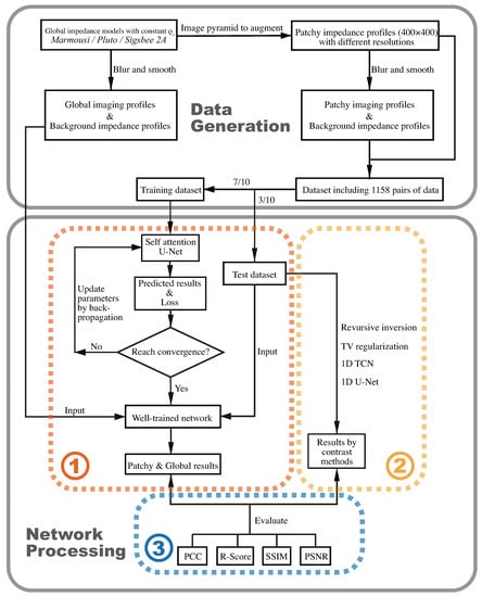 Figure 3. Complete workflow: Including two parts, data generation, and network processing. Network processing has three steps: training, validating, and evaluating.
3. Experiments
3.1. Dataset
3.1.1. Data Augment
First, the impedance profiles with consistent density but different resolutions are obtained by the pyramid method. Second, a square window strides on these profiles to crop, and patches with local or global impedance features but the same shape are obtained. The Marmousi, Pluto, and Sigsbee 2A [,,] profiles with P-wave speed and consistent density shaped by (2801, 13,601), (1201, 6960), and (1201, 3201), respectively, are resampled to (400, 400). Finally, there are 1158 profiles with P-wave speed and consistent density in this paper. A profile is shown in Figure 4a.
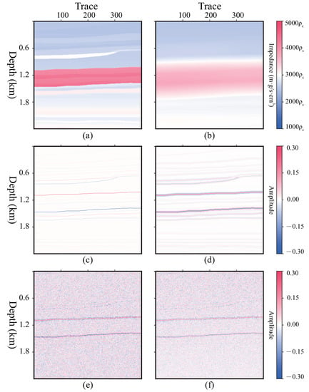
Figure 4.
Dataset generation. (a) Impedance profile with constant density , (b) background impedance , (c) reflection coefficient profile , (d) seismic profile with convolution by K = 0.030, P = 0 Ricker wavelet, (e) seismic profile with = −5.00dB, (f) seismic profile with linear attenuation.
3.1.2. Background Impedance Profile
Smoothing each impedance profile by Gaussian filter with kernel size as 100 aims to generate the background impedance profile , shown in Figure 4b.
3.1.3. Seismic Profile
According to (1) and an impedance profile in Figure 4a, the reflection coefficient profile (Figure 4c) in the spatial vertical direction can be calculated from . The Ricker wavelet in the spatial domain with a random phase P ranged [−60, 60] and a random wave number K in the range of [10, 40]∗10 (m) is convolved with to obtain profile (Figure 4d), i.e., wavelet fuzzification. To simulate the field survey, random noise has been added to and the noisy profile (Figure 4e) is available for our further tests. Making the signal-to-noise ratio () of all conform to the positive-skewed distribution with a skewness coefficient is about 0.075. The distributions of these three factors are shown in Figure 5. Considering the energy attenuation since seismic wave propagation, the amplitude of attenuates with depth linearly. The amplitude of the deepest layer is 0.5 times the original amplitude. Finally, the seismic profile shown in Figure 4f is generated.
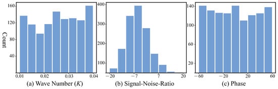
Figure 5.
Distributions of wavelet factors, (a) K conform to a uniform distribution, (b) conform to positive-skewed distribution because the energy of the noise is commonly stronger than the signal in the field cases, (c) P conform to a uniform distribution.
Each impedance profile calculates a background impedance profile and a seismic profile . is label data, and are channel 1st and 2nd of input data, respectively. Such corresponding , and is a pair of data. The dataset has a total of 1158 pairs in this paper, which is divided into the training dataset and the test dataset by 7:3 and no cross-validation, i.e., the test dataset absolutely does not contribute to training.
3.2. Convergence
Training is terminated after 300 epochs (i.e., 1158 × 0.7 × 300 = 243,300 iterations), and the convergent curve of loss value is shown in Figure 6. To validate this method concretely, Figure 7 validates convergence by outputs at different epochs. From Figure 6 and Figure 7d, the loss is relatively low at 50 epochs, but the impedance profile is blurry at details of high frequency. With more training epochs, the network could predict the wide-band impedance profile shown in Figure 7e, which is close to the label shown in Figure 7f.
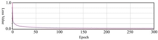
Figure 6.
Loss curve in training. It illustrates that the loss was gradually minimized by training and became stable after 50 epochs. It basically got convergence after 300 epochs.
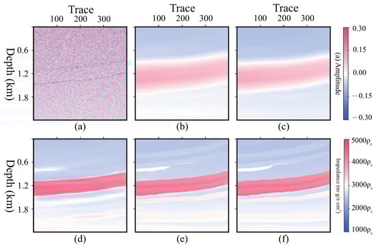
Figure 7.
Predicted profiles at different epochs. (a) , channel 1 of input data, (b) , channel 2 of input data, (c) predicted profile at 10 epoch, (d) predicted profile at 50 epoch, (e) predicted profile at 300 epoch, (f) label profile .
4. Results
4.1. Patchy Profiles
The test dataset includes a total of 347 profiles; 2 of the test results and their wavenumber spectrums are shown in Figure 8, Figure 9, Figure 10 and Figure 11. It is a part of Marmousi, including shallow horizontal layers and deep faults. To validate that this network could extend the band of wavenumber, we utilized Fourier transform to test the results to obtain the wavenumber spectrums, which are given in Figure 9 and Figure 11.
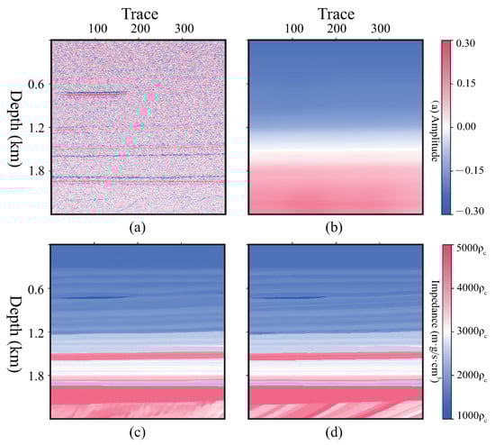
Figure 8.
A profile from the test dataset. (a) , channel 1 of input data, K = 0.015, = −4.72 dB, P = 10, (b) , channel 2 of input data, (c) predicted profile , PCC = 0.9924, R = 0.8393, SSIM = 0.8984, PSNR = 27.71 dB. (d) label profile .
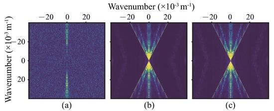
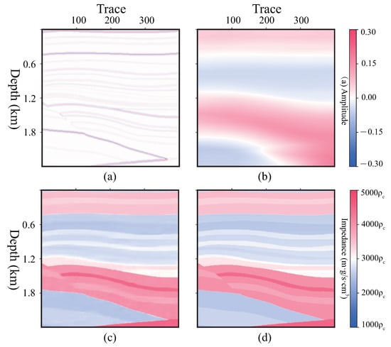
Figure 10.
A profile from the test dataset. (a) , channel 1 of input data, K = 0.027, = 3.57 dB, P = −11 , (b) , channel 2 of input data, (c) predicted profile , PCC = 0.9935, R = 0.9427, SSIM = 0.9536, PSNR = 28.04 dB. (d) label profile .
4.2. Global Profiles
4.2.1. Standard Seismic Models
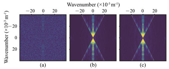
As introduced above, the network in this paper is flexible and not limited by the shape of inputs. It is trained by patchy profiles and is able to process a whole profile that has different shapes from patches. Figure 12, Figure 13 and Figure 14 show the test results of the global profiles, Marmousi, Pluto, and Sigsbee 2A respectively, and illustrate that this method is effective for predicting accurate impedance from a seismic profile and background impedance profile. We selected three single traces, No. 3500, 8680, and 12,200, from Marmousi. The black lines stand for label data and the red stand for our results in Figure 15.
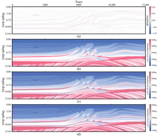
Figure 12.
Test result of the Marmousi profile, (a) , K = 0.034, = 5.00 dB, P = −9, channel 1 of input data, (b) , channel 2 of input data, (c) predicted profile , PCC = 0.9813, R = 0.7994, SSIM = 0.9081, PSNR = 23.96 dB. (d) label profile .
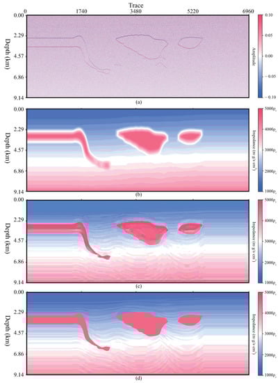
Figure 13.
Test result of the Pluto profile, (a) , K = 0.039, = −5.00 dB, P = 50, channel 1 of input data, (b) , channel 2 of input data, (c) predicted profile , PCC = 0.9678, R = 0.7717, SSIM = 0.8972, PSNR = 22.03 dB. (d) label profile .
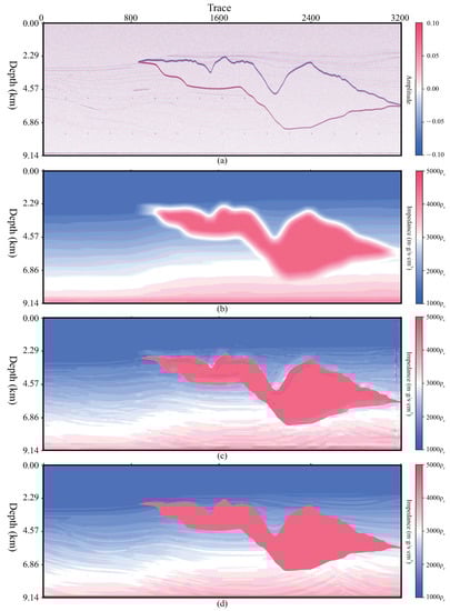
Figure 14.
Test result of the Sigsbee 2A profile, (a) , K = 0.017, = 0.00 dB, P = 41, channel 1 of input data, (b) , channel 2 of input data, (c) predicted profile , PCC = 0.9684, R = 0.8703, SSIM = 0.7286, PSNR = 21.11 dB. (d) label profile .
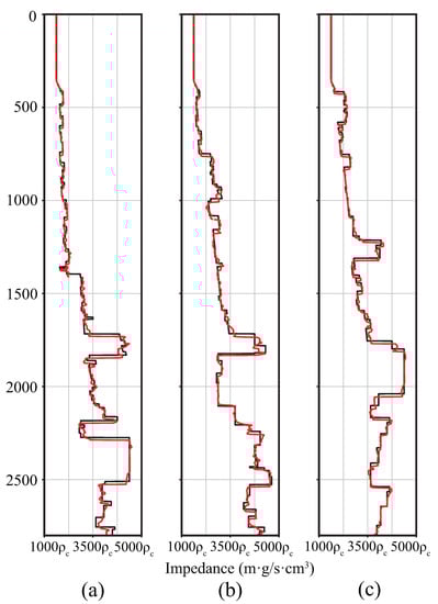
Figure 15.
The predicted (red) and true (black) impedance of a single trace (a) No. 3500, (b) 8680, and (c) 12,200, from Marmousi.
4.2.2. Field Case: EPP 39 and EPP40 Ceduna Survey
To illustrate the generalization of self-attention U-Net, a further experiment is performed on a 3D field dataset [] without any labels. This dataset is from Equinor, which is the sole titleholder of exploration permit 39 (EPP39). As part of the permit commitment, Equinor plans to drill the Stromlo-1 exploration well. The well is located in the Ceduna sub-basin off southern Australia, which is approximately 400 km southwest of Ceduna and 476 km west of Port Lincoln, at a water depth of 2240 m. Equinor Australia B.V. shares the 3D migration velocity and migrations dataset []. The size of the dataset is 1201 (depth) × 1007 (crossline) × 1481 (inline). The spacing interval of the depth is 10 m. Two slices in inline are given in Figure 16 and Figure 17, respectively. The input of this case is the migration slice (a) as channel 1 and velocity slice (b) as channel 2. The corresponding outputs by the network are shown in (c). In order to illustrate the details of the structure, (d)–(f) display the corresponding magnified area, which are marked by white dashed boxes in (a)–(c), respectively.
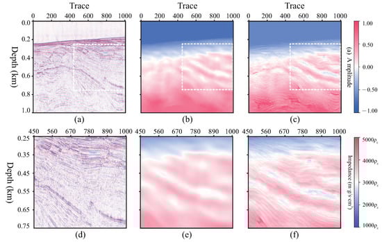
Figure 16.
Result of inline No.550 slice. (a) The migrations. (b) The background impedance with constant density. (c) The prediction by self-attention U-Net. (d–f) The zoomed-in area of (a–c).
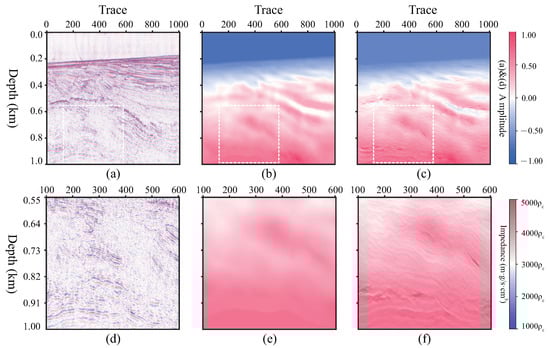
Figure 17.
Result of inline No.750 slice. (a) The migrations. (b) The background impedance. (c) The prediction. (d–f) The zoomed-in area of (a–c).
5. Discussion
5.1. Analysis of the Results
Combining Figure 8c,d and Figure 10c,d, the method in this paper can predict accurate impedance with blurred seismic profile and background impedance. The edges and faults in subfigure (c) are smoother than subfigure (d) because of optimization. From wavenumber spectrums, Figure 10a and Figure 11a, the input data are band-limited and contaminated by noise. The spectrums of the predicted profiles, Figure 10b and Figure 11b, are much clearer than the input and close to the spectrums of the labels. It validates that our method can predict impedance rationally and broadens the wavenumber band.
Index changes before (X-axis) and after (Y-axis) processed by self-attention U-Net are shown in Figure 18. The index values located above the Y = X lines are marked by grey lines in these subfigures. This illustrates that our method works effectively.
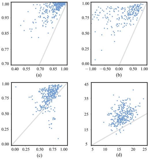
Figure 18.
Index values before (X-axis) and after (Y-axis) processed by self-attention U-Net. (a) PCC, (b) R, (c) SSIM, (d) PSNR.
For the results of standard seismic models, Figure 12, Figure 13, Figure 14 and Figure 15 illustrate that our method could predict impedance accurately from both phase and amplitude. Not only the bone of the low wavenumber but also the details of the high wavenumber are recovered by the proposed network.
For the results of the field dataset, Figure 16 and Figure 17 demonstrate the correctness and effectiveness of the proposed method in recovering the stratigraphic details. As seen in Figure 17f, even for some deep areas, the network can predict a clear and reasonable impedance profile. On account of having no accurate impedance model of the target area, this paper could only give some subjective and abstract analysis of these results. As we could see from the comparisons in Figure 16 and Figure 17, our proposed training strategy demonstrates its potential to deal with field datasets without any labels in advance. This is because the image pyramid could augment the impedance dataset, which is beneficial to network training. In addition, the Pluto and the Sigsbee models enrich the generalization ability of our network.
5.2. Self-Attention Analysis
To validate the self-attention block, it is helpful to improve the predicted result by U-Net. Figure 19 shows the loss curves. It illustrates that U-Net tends to become convergent by less training epoch than with the self-attention block. The predicted profiles are shown in Figure 20. It obviously illustrates that the self-attention U-Net recovered a low-speed body, which is marked by white dashed boxes. Subfigure (b) shows the higher values of all indices, which prove that the result obtained by self-attention U-Net is more similar to the label and has less noise than the one without the self-attention block.
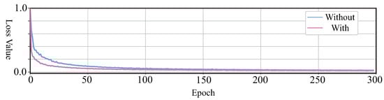
Figure 19.
Loss curve in training with and without the self-attention block.
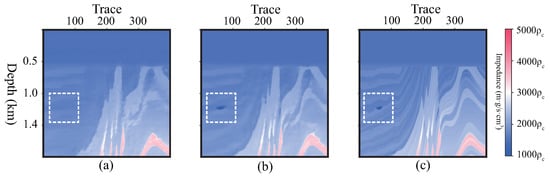
Figure 20.
Self-attention contrast. (a) The result processed without the self-attention block, PCC = 0.9787, R = 0.9004, SSIM = 0.4375 PSNR = 14.99 dB. (b) The result processed with the self-attention block, PCC = 0.9867, R = 0.9376, SSIM = 0.8589, PSNR = 30.06 dB. (c) The label data.
5.3. Comparative Analysis
5.3.1. Deconvolution and Recursive Inversion
A result of deconvolution and recursive inversion is shown in Figure 21. This method requires a seismic imaging profile and seismic wavelet. The predicted profile is shown in subfigure (b), and errors are generated. It is absolutely inaccurate in the following integration to calculate the impedance profile. There is a problem regarding the energetic imbalance for 1D inversion.
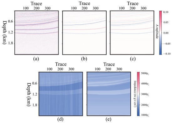
Figure 21.
Profiles of deconvolution and recursive inversion. (a) Seismic profile , (b) profile by deconvolution, (c) profile, (d) profile by recursive inversion, (e) profile.
5.3.2. TV Regularization Inversion
A result of TV regulation is shown in Figure 22. This method needs a seismic profile, initial (background) impedance profile, and a seismic wavelet. It is affected by the quality of the initial impedance. Subfigure (b) is the initial impedance, subfigure (c) is noisy and does not sharpen the edges. Subfigure (e) is the initial impedance and subfigure (f) is clearer and sharper. However, field surveys hardly have such accurate background impedance.
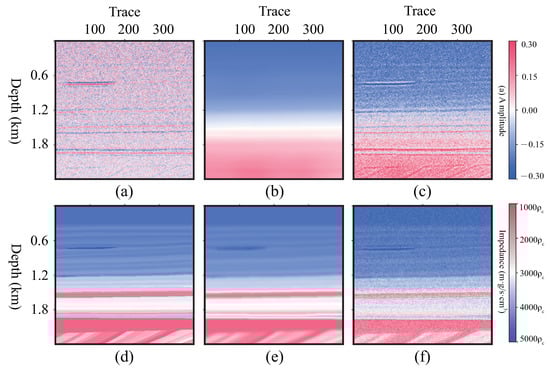
Figure 22.
Profiles of TV regularization. (a) , seismic profile, (b) , background impedance profile, smooth filter size = 100, (c) predicted profile by (a,b), (d) label profile , (e) , background impedance profile, smooth filter size = 10, (c) predicted profile by (a,e). (f) predicted profile by (a,e).
5.3.3. 1D Neural Network
We selected a case, as shown in Figure 23, to illustrate that our method is better than conventional methods and 1D network methods. These are the results of TCN [13] and 1D U-Net in Figure 23e,f. It failed to accurately recover the impedance value by recursive inversion in subfigure (c). TV regularization in subfigure (d) cannot give accurate locations of interfaces TCN, and can only capture the background impedance in subfigure (e). 1D U-Net generated some errors in subfigure (f). The profile in subfigure (g) that is predicted by the self-attention U-Net is clear and close to the label data in subfigure (h).
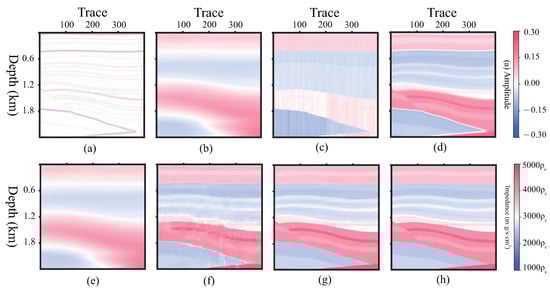
Figure 23.
Profiles. (a) , seismic profile, (b) , background impedance profile, (c) predicted by deconvolution and recursive inversion, (d) predicted by TV regularization, (e) predicted by TCN, (f) predicted by 1D U-Net, (g) predicted by self-attention U-Net, (h) label profile .
6. Conclusions
This research combined U-Net with self-attention and mapped the characters from a seismic imaging profile to an impedance profile. Based on the image pyramid used to augment the label data, and the seismic convolution model used to generate the input data, 1158 pairs of patchy imaging profiles were used for training and testing. After about 300 epoch iterations, the network reached convergence and predicted the accurate impedance profiles. We valued the output’s quality by four indexes, PCC, R, SSIM and PSNR. It proved that this method is effective and reasonable.
In contrast, the self-attention block did improve the predicted results. Compared with deconvolution with recursive inversion, regularization and 1D network method, the 2D neural network shows better spatial continuity and accurate value of impedance.
Furthermore, tests on complete global seismic profiles are effective since the self-attention U-Net is a fully convolutional network. The predictions of field data illustrate that the network can be generalized from a synthetic dataset to a field dataset without labels. It proves the potentiality of this strategy, which could be extended to scenarios of field surveys.
Author Contributions
Conceptualization, methodology, resources, and formal analysis, L.T., H.R. and Z.G.; software, validation, and data curation, L.T. and Z.G.; writing—original draft preparation, L.T.; writing—review and editing, Z.G. and H.R.; visualization, L.T.; supervision, H.R.; project administration, L.T. and H.R.; funding acquisition, H.R. All authors have read and agreed to the published version of the manuscript.
Funding
This research was funded by the National Natural Science Foundation of China grant No. 42074135 and 41874164; by the Project of Sanya Yazhou Bay Science and Technology City grant No. SCKJ-JYRC-2022-45 and SCKJ-JYRC-2022-46.
Data Availability Statement
Not applicable.
Conflicts of Interest
The authors declare no conflict of interest. The funders had no role in the design of the study; in the collection, analyses, or interpretation of data; in the writing of the manuscript; or in the decision to publish the results.
References
- Cooke, D.A.; Schneider, W.A. Generalized linear inversion of reflection seismic data. Geophysics 1983, 48, 665–676. [Google Scholar] [CrossRef]
- Connolly, P. Elastic impedance. Lead. Edge 1999, 18, 438–452. [Google Scholar] [CrossRef]
- Shuey, R.T. A simplification of the Zoeppritz equations. Geophysics 1985, 50, 609–614. [Google Scholar] [CrossRef]
- Gholami, A. Nonlinear multichannel impedance inversion by total-variation regularization. Geophysics 2015, 80, R217–R224. [Google Scholar] [CrossRef]
- Dossal, C.; Mallat, S. Sparse spike deconvolution with minimum scale. Proc. Signal Process. Adapt. Sparse Struct. Represent. 2005, 4, 4–7. [Google Scholar]
- Luo, Y.; Schuster, G.T. Wave-equation traveltime inversion. Geophysics 2015, 56, 645–653. [Google Scholar] [CrossRef]
- Jiang, J.; Ren, H.; Zhang, M. A Convolutional Autoencoder Method for Simultaneous Seismic Data Reconstruction and Denoising. IEEE GRSL 2022, 19, 1–5. [Google Scholar] [CrossRef]
- Tao, L.; Ren, H.; Ye, Y.; Jiang, J. Seismic Surface-Related Multiples Suppression Based on SAGAN. IEEE GRSL 2022, 19, 3006605. [Google Scholar] [CrossRef]
- He, X.; Zhou, Y.; Zhao, J.; Zhang, D.; Yao, R.; Xue, Y. Swin Transformer Embedding UNet for Remote Sensing Image Semantic Segmentation. IEEE TGRS 2022, 60, 1–15. [Google Scholar] [CrossRef]
- Cui, S.; Ma, A.; Zhang, L.; Xu, M.; Zhong, Y. MAP-Net: SAR and Optical Image Matching via Image-Based Convolutional Network With Attention Mechanism and Spatial Pyramid Aggregated Pooling. IEEE TGRS 2022, 60, 1–13. [Google Scholar] [CrossRef]
- Gadylshin, K.; Vishnevsky, D.; Gadylshina, K. Numerical dispersion mitigation neural network for seismic modeling. Geophysics 2022, 87, T237–T249. [Google Scholar] [CrossRef]
- Das, V.; Pollack, A. Convolutional neural network for seismic impedance inversion. Geophysics 2019, 84, R869–R880. [Google Scholar] [CrossRef]
- Mustafa, A.; Alfarraj, M.; AlRegib, G. Estimation of Acoustic Impedance from Seismic Data using Temporal Convolutional Network. In Expanded Abstracts of the SEG Annual Meeting; Society of Exploration Geophysicists: Houston, TX, USA, 2019; pp. 15–20. [Google Scholar]
- Wang, Y.; Wang, Q.; Lu, W.; Li, H. Physics-Constrained Seismic Impedance Inversion Based on Deep Learning. IEEE GRSL 2022, 19, 7503305. [Google Scholar] [CrossRef]
- Gao, Z.; Yang, W.; Tian, Y.; Li, C.; Jiang, X.; Gao, J.; Xu, Z. Global optimization with deep-learning-based acceleration surrogate for large-scale seismic acoustic-impedance inversion. Geophysics 2022, 87, R35–R51. [Google Scholar] [CrossRef]
- Wu, X.; Yan, S.; Bi, Z.; Zhang, S.; Si, H. Deep learning for multidimensional seismic impedance inversion. Geophysics 2021, 86, R735–R745. [Google Scholar] [CrossRef]
- Yuan, S.; Wang, S.; Luo, Y.; Wei, W.; Wang, G. Impedance inversion by using the low-frequency full-waveform inversion result as an a priori model. Geophysics 2019, 82, R149–R164. [Google Scholar] [CrossRef]
- Wu, B.; Meng, D.; Wang, L.; Liu, N.; Wang, Y. Seismic impedance inversion using fully convolutional residual network and transfer learning. IEEE GRSL 2020, 17, 2140–2144. [Google Scholar] [CrossRef]
- Sun, J.; Innanen, K.A.; Huang, C. Physics-guided deep learning for seismic inversion with hybrid training and uncertainty analysis. Geophysics 2021, 86, R303–R317. [Google Scholar] [CrossRef]
- Wang, L.; Meng, D.; Wu, B. Seismic inversion via closed-loop fully convolutional residual network and transfer learning. Geophysics 2021, 86, R671–R683. [Google Scholar] [CrossRef]
- Wu, B.; Meng, D.; Zhao, H. Semi-supervised learning for seismic impedance inversion using generative adversarial networks. Remote Sens. 2021, 13, 909. [Google Scholar] [CrossRef]
- Aleardi, M.; Salusti, A. Elastic prestack seismic inversion through discrete cosine transform reparameterization and convolutional neural networksDCT-CNN prestack elastic inversion. Geophysics 2021, 86, R129–R146. [Google Scholar] [CrossRef]
- Jaderberg, M.; Simonyan, K.; Zisserman, A.; Kavukcuoglu, K. Spatial transformer networks. In Proceedings of the 28th International Conference on Neural Information Processing Systems, Montreal, QC, Canada, 5–12 December 2015; Volume 2, pp. 2017–2025. [Google Scholar]
- Ronneberger, O.; Fischer, P.; Brox, T. U-Net: Convolutional Networks for Biomedical Image Segmentation. MICCAI 2015, 9351, 234–241. [Google Scholar]
- Gary, S.M.; Robert, W.; Kurt, J.M. Marmousi2: An elastic upgrade for Marmousi. Lead. Edge 2006, 25, 156–166. [Google Scholar]
- Wu, B.; Xie, Q.; Wu, B. Seismic Impedance Inversion Based on Residual Attention Network. IEEE Trans. Geosci. Remote Sens. 2022, 60, 1–17. [Google Scholar] [CrossRef]
- Sigsbee2 Models. Available online: https://reproducibility.org/RSF/book/data/sigsbee/paper.pdf (accessed on 26 April 2022).
- Released Documents of NOPIMS. Available online: https://nopims.dmp.wa.gov.au/Nopims/Search/ReleasedDocuments (accessed on 24 November 2022).
- Information about Stromlo-1 Exploration Drilling Program. Available online: https://info.nopsema.gov.au/environment_plans/463/show_public (accessed on 24 November 2022).
Disclaimer/Publisher’s Note: The statements, opinions and data contained in all publications are solely those of the individual author(s) and contributor(s) and not of MDPI and/or the editor(s). MDPI and/or the editor(s) disclaim responsibility for any injury to people or property resulting from any ideas, methods, instructions or products referred to in the content. |
© 2023 by the authors. Licensee MDPI, Basel, Switzerland. This article is an open access article distributed under the terms and conditions of the Creative Commons Attribution (CC BY) license (https://creativecommons.org/licenses/by/4.0/).