Biases’ Characteristics Assessment of the HY-2B Scanning Microwave Radiometer (SMR)’s Observations

Abstract

The second Chinese ocean dynamic environment satellite Haiyang-2B (HY-2B), carrying a scanning microwave radiometer (SMR) to provide information on the ocean and atmosphere, was successfully launched on 25 October 2018. Before the data assimilation, it is necessary to characterize and evaluate the biases of the HY-2B SMR observations. This study is the first to conduct a systematic assessment of the SMR radiance data based on observation minus background simulation (O-B). Three types of numerical weather prediction (NWP) datasets, including ECMWF Reanalysis v5 (ERA5), the analysis fields from the NCEP Global Forecast System (NCEP-GFS), and the analysis fields from the Global Regional Assimilation and Prediction System-Global Forecast System (GRAPES-GFS), were used as input information for RTTOV v12.3 to simulate the SMR’s observed brightness temperature (TB) under clear-sky conditions. Study results showed that the O-B biases and IQR of the SMR for most channels were within −2.5–0.4 K and smaller than 4 K, respectively. The SMR observations were generally consistent with the RTTOV simulations, even based on the different NWP fields. These results indicate a good prospect for the assimilated application of HY-2B SMR radiance data. However, due to the impact of RFI, the SMR’s descending data for two 10.7 GHz channels showed some significant positive biases larger than 50 K over the seas of the European region. In addition, it seems that the bias characteristics of the SMR’s ascending data were obviously different from those of the descending data. It was also found that the variation trend of scan-position-dependent bias was generally stable for the SMR’s ascending data but fluctuates significantly for the descending data, with a maximum amplitude greater than 0.7 K for some channels.

1. Introduction

Satellite radiance observations have become the dominant sources of ocean, land, and atmospheric information in both regional and global numerical weather prediction (NWP) systems [1]. Most global NWP systems rely on satellite radiance data assimilation to depict the best initial value of the model [2,3,4]. Recent studies have shown that the observations from microwave imagers show great potential to improve the analysis of atmospheric information and the forecasts of micro-scale weather systems [5,6,7]. For instance, the assimilation of Feng Yun-3C (FY-3C) Microwave Radiation Imager (MWRI) radiance data had a positive effect on the geopotential height and humidity analysis in the Global Regional Assimilation and Prediction System-Global Forecast System (GRAPES-GFS), leading, for example, to improvements in the forecasts of Typhoon Shanshan’s track [8]. Kazumori et al. [9] evaluated the observations from three microwave imagers in terms of Advanced Microwave Scanning Radiometer-2 (AMSR2), Special Sensor Microwave Imager/Sounder (SSMIS), and TRMM Microwave Imager (TMI) in the ECMWF system. It was also proven that the humidity, temperature, and surface wind could be adjusted by all of these microwave imagers’ observations. Similarly, more precise information on the geopotential height could be provided by the GPM microwave imager (GMI), which is essential for the forecasts of Typhoon “Chan-Hom” [10].

The second Chinese ocean dynamic environment satellite, Haiyang-2B (HY-2B), was successfully launched on 25 October 2018. The HY-2B satellite is operated at a 967 km altitude sun-synchronous orbit with a local equator crossing time (LECT) of 6:00 A.M. (descending) [11]. HY-2B is equipped with four microwave instruments: a scanning microwave radiometer (SMR), a microwave scatterometer (SCA), a dual-frequency radar altimeter (ALT), and a calibration microwave radiometer (CMR) [11]. Currently, the HY-2B SMR has become the only microwave imager to operate in the early morning (EM) orbit for civil use. It is worth mentioning that polar-orbiting satellites can be classified into three types according to their different LECTs in the descending orbit, including morning satellites (at around 10 LECT), afternoon satellites (at around 14 LECT), and early morning satellites (at around 6 LECT) [12]. As shown in Figure 1, over seventy percent of the global coverage could be achieved every 6 h by the HY-2B SMR jointed with MWRIs onboard the FY-3C/D satellites. Furthermore, some efforts have been made on radiometric calibration [13], the initial evaluation of early in-orbit performance [14,15], and the assessments of retrieval products [16,17], demonstrating that the high-quality SMR radiance data are made available for weather monitoring. The assimilation of the SMR radiance data has the potential capability to provide a better analysis and forecast of atmospheric variables.

Data assimilation systems are developed based on the assumption of unbiased Gaussian observational errors. Therefore, assessing the biases of satellite radiance data is a crucial prerequisite for data assimilation [18]. A widely adopted approach for the instrumental bias estimate is to quantify the departures between the observed and simulated brightness temperature (O-B). Lawrence et al. [19] analyzed the O-B statistics to characterize the biases of FY-3C MWRI and found an ascending-minus-descending (AD) bias around 2 K in both the ECMWF and Met Office systems. These AD biases could be effectively modified by the physical-based correction algorithm proposed by Xie et al. [20]. Based on the above achievements, the FY3-C/D MWRIs’ observations have been directly assimilated into the Met Office and CMA assimilation systems [8,21]. A similar approach was also applied for the evaluation of AMSR2 observations. It was proven that the low-frequency channels of AMSR2 are affected by sun glint in some areas [9]. In addition, the assessment of DMSP F-18 SSMIS observations demonstrated that the large biases of lower atmospheric sounding channels are dependent on the swaths, seasons, and latitudes [22]. However, there is still less research concerning the assessment of bias characteristics for SMR radiance data. In fact, the SMR bias characteristics depicted by the different NWP fields have not yet been researched.

This study is the first attempt to evaluate the bias characteristics of HY-2B SMR observations based on O-B. Moreover, different bias characteristics of SMR are discussed based on the three NWP fields in terms of the ECMWF Reanalysis v5 (ERA5), the analysis fields from the NCEP Global Forecast System (NCEP-GFS), and the analysis fields from the Global Regional Assimilation and Prediction System-Global Forecast System (GRAPES-GFS).

The remainder of this paper is organized as follows. Section 2 introduces the instrumental details of the SMR, the datasets used in this study, the fast radiative transfer models for SMR simulations, as well as the quality control method. Section 3 presents the results of the SMR’s systematic evaluation. Finally, the discussion and conclusions are summarized in Section 4.

2. Materials and Methods

2.1. HY-2B SMR Characteristic

As a 9-channel conical-scanning radiometer, the HY-2B SMR scans the earth over a swath width of 1600 km with a scan angle of 53.15°. Excluding 23.8 GHz, the other four frequencies of SMR have vertical and horizontal polarization channels. The footprint sizes of each frequency differ from one another, and the higher the frequency, the smaller the footprint (

Table 1. Instrument specifications of SMR.

Center Frequency (GHz)	Band Width (MHz)	Polarization	Footprint Sizes (km × km)	NEDT (K)	Main Application
6.925	350	V\H	73 × 109	≤0.5	Sea surface temperature
10.7	100	V\H	55 × 82	≤0.6	Sea surface wind speed
18.7	200	V\H	33 × 55	≤0.5	Ocean rain
23.8	400	V	28 × 47	≤0.5	Atmospheric water vapour
37.0	1000	V\H	19 × 31	≤0.8	Cloud liquid water

). Figure 2 shows the weighting functions and humidity Jacobian functions of all SMR channels calculated by RTTOV with the American Standard atmosphere profile as input. It can be seen that the channels at 6.925 GHz and 10.7 GHz are more transparent to the atmosphere (Figure 2a). Thus, these channels are typically used to detect surface variables, such as the sea surface temperature and sea surface wind speed. The other five channels, ranging from 18.7 GHz to 37 GHz, are sensitive to low-level humidity, with a peak located at around 800–900 hPa (Figure 2b). Additionally, the 18.7 GHz and 37 GHz channels also involve the retrieval applications of ocean rain and cloud liquid water content, respectively.

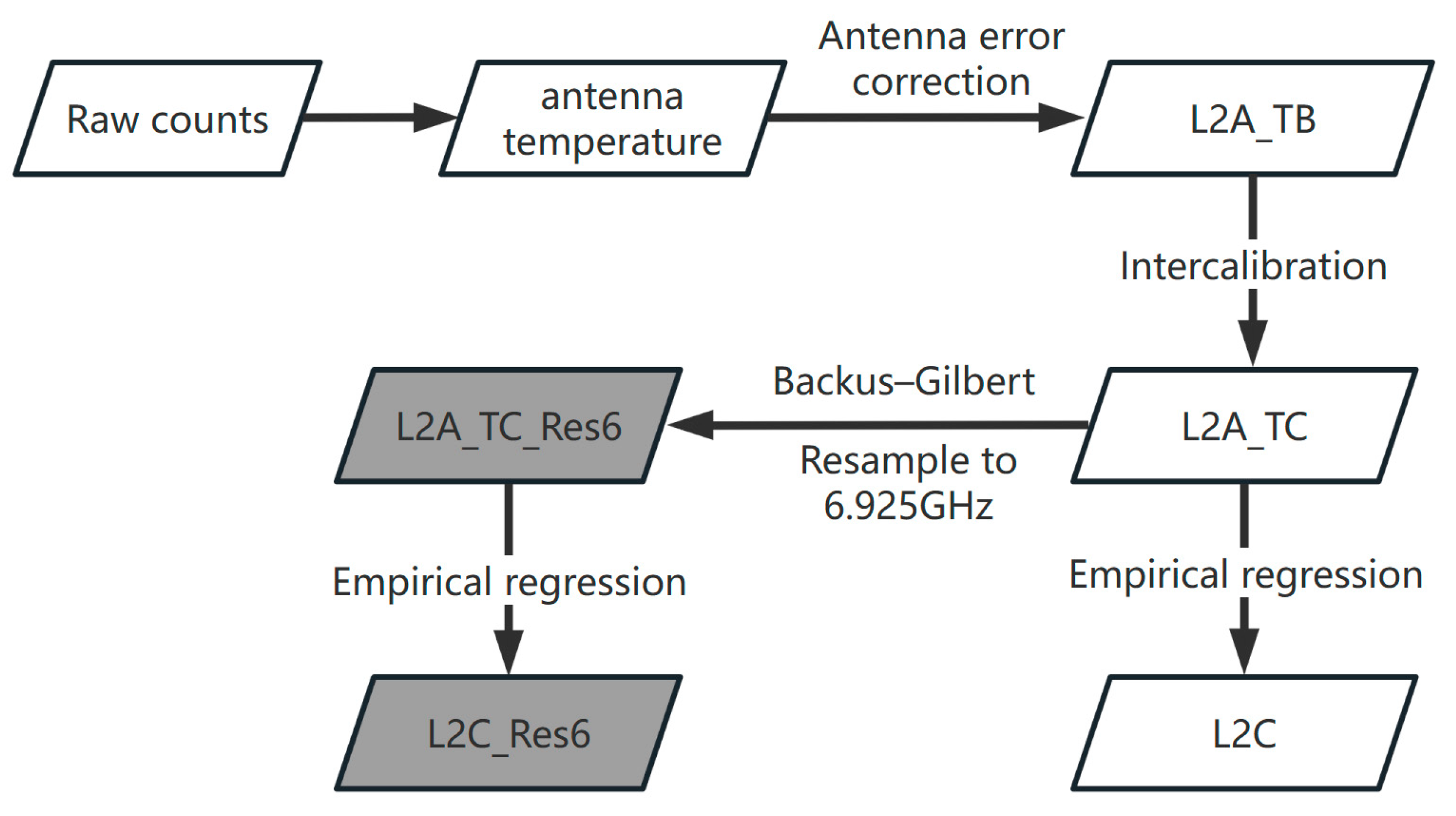
2.2. HY-2B SMR Radiance Data

Figure 3 shows the basic flowchart of data processing for HY-2B SMR. The raw counts observed by SMR are converted into antenna temperatures, which are then converted to brightness temperature (TB) through some necessary corrections, such as antenna error correction. This level of SMR data is called L2A_TB. Then, the National Satellite Ocean Application Service (NSOAS) data processing center uses L2A_TB datasets to conduct inter-calibration with other microwave imager observations [23,24] and model-calculated results [25]. These product results are called L2A_TC, which have a smaller annual drift and better stability compared with the L2A_TB datasets, with annual drifts of TBs less than 0.1 K per year [26]. Moreover, in order to retrieve the precise geophysical parameters from multi-frequency TBs, the original resolution of radiance datasets (L2A_TC_Res0) was spatially resampled to the resolution of 6.925 GHz (L2A_TC_Res6) based on the Backus–Gilbert (BG) method. The L2A_TC_Res6 swath archive datasets are half-orbital (ascending/descending separated), time-ordered, and geolocated; they contain the resampled TBs, full geolocation information, and satellite observation geometry. In this study, the HY-2B L2A_TC_Res6 swath datasets offered by the NSOAS are used to evaluate the SMR observations from 10 July 2021 to 10 August 2021. Additionally, one-month datasets of L2A_TC_Res6 from 10 January 2021 to 10 February 2021 have been applied to evaluate the seasonal variation in SMR AD bias. The corresponding retrieved product, named L2C_Res6, was also applied for the data quality control (QC) procedures.

2.3. Radiative Transfer Model and Ocean Emissivity Model

In this study, the RTTOV v12.3 supported by the EUMETSAT NWP Satellite Application Facility (NWP SAF) was adopted as a forward radiative transfer model to simulate the SMR-observed TB values under clear-sky conditions.

Table 2. Input parameters of RTTOV.

Category	Parameter	Unit	Data Resource
Atmosphere profiles	Pressure	hPa	NWP fields
	Temperature	K
	Specific humidity	kg/kg
Surface variables	Surface temperature	K	NWP fields
	Surface pressure	hPa
	2 m temperature	K
	2 m specific humidity	kg/kg
	10-m u component	m/s
	10-m v component	m/s
	Land–sea mask	-	Satellite
	Ocean surface emissivity	-	Fastem-6
Geometry	Latitude	Degrees	Satellite
	Longitude	Degrees
	Satellite zenith angle	Degrees
	Satellite azimuth angle	Degrees
	Terrestrial elevation	m	0 for ocean

summarizes the detailed description of the input variables for RTTOV.

The ocean surface emissivity was calculated by the Fast Emissivity Modeling (FASTEM) version 6. Currently, Fastem-6 is applied for major NWP centers up to 200 GHz and yields realistic estimates of the sea surface emissivities [27,28].

2.4. Quality Control Procedures

Data quality control (QC) procedures should be carried out before the instrument performance assessments and the applications. The data of no interest, such as cloud-polluted data or questionable data, should be effectively filtered by QC procedures [29]. The QC procedures for SMR radiance data consist of six steps, as follows:

• An abnormal value check, which deletes observations with TB < 50 or >350 K.
• A surface-type check. Data over land are discarded because of the uncertainties of land surface emissivity.
• A latitude check, keeping only data between 50°N and 50°S to avoid including the pixels over sea ice.
• Cloud detection. Only clear sky pixels are retained due to the uncertainty arising from the known deficiencies of the radiance transfer model (RTM) in the cloud/precipitation regions as well as the inaccurate location of the hydrometeors. Three processes are used here to reject the cloudy affected pixels:

  1.

  The observation is retained only if $T{B}_V^{37}-T{B}_H^{37}>50\mathrm{K}$ [8].

  2.

  Data are rejected if the cloud liquid water path (CLWP) values in the L2C_Res6 products are larger than 0.05 kg/m².

  3.

  The observation is retained only if $C_{37}^o<0.05$ [19]. The observation cloud amount $C_{37}^o$ is calculated as follows:

  $$P_{37}^o=(T{B}_V^o-T{B}_H^o)/(T{B}_{\mathrm{V}}^b-T{B}_H^b),$$

  (1)

  $$C_{37}^o=1-P_{37}^o,$$

  (2)

  where $P_{37}^o$ is the normalized polarization difference at 37 GHz channels. $T{B}_V^o$ and $T{B}_H^o$ are the 37 GHz V and H polarization observations, respectively. $T{B}_{\mathrm{V}}^b$ and $T{B}_H^b$ are the simulated TBs for these channels.

5.

A rain rate check. Rain is assumed if the data meet any of the following conditions [30,31]:

$$T{B}_{\mathrm{V}}^{37}-0.979T{B}_{\mathrm{H}}^{37}<55\mathrm{K},$$

(3)

$$1.175T{B}_{\mathrm{V}}^{18.7}-30>T{B}_{\mathrm{V}}^{37},$$

(4)

$$T{B}_{\mathrm{H}}^{18.7}>170\mathrm{K},$$

(5)

$$T{B}_{\mathrm{H}}^{37}>210\mathrm{K}.$$

(6)

6.

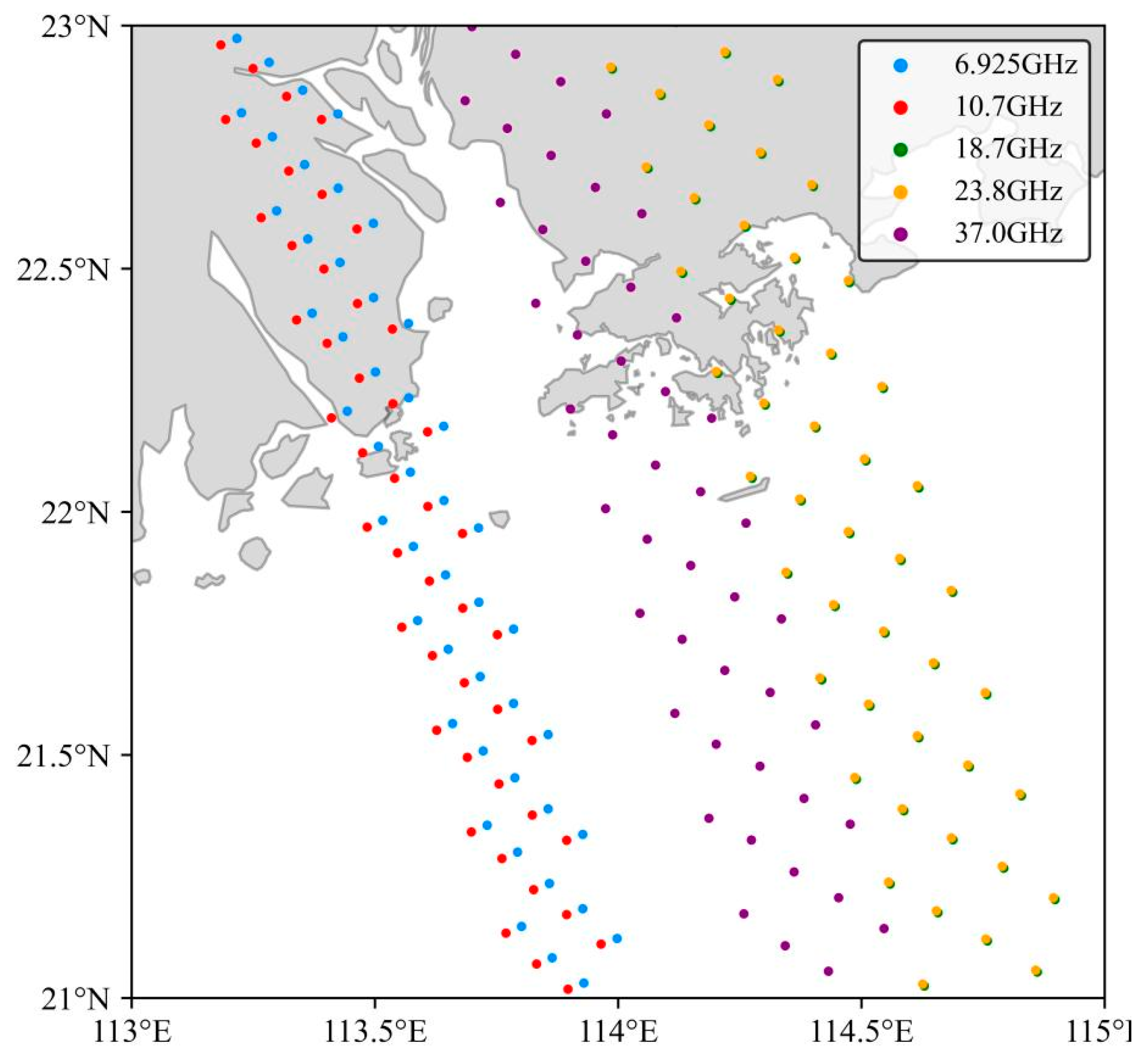
A scan position check. Figure 4 shows the spatial distribution of the first five pixels of the SMR between different frequencies ranging from 6.925 GHz to 37 GHz. It can be seen that there are significant discrepancies in the distribution of pixels between the different frequencies (Figure 4), which is mainly due to the SMR using three feedhorns to receive radiation signals ranging from 6.925 GHz to 37 GHz. Due to this difference in the location of each frequency’s pixel, some of the SMR pixels would be lost after resampling to the resolution of 6.925 GHz, and the available pixels are not consistent between different frequencies (

Table 3. Threshold of CLWP and available pixels after resampling to 6.925 GHz.

Frequency (GHz)	Available Pixels
6.925	1–150
10.7	6–145
18.7	18–150
23.8	18–150
37.0	14–150

). In order to equalize the number of SMR pixels with different frequencies, the first 17 pixels and the last 5 pixels for all channels of the SMR are discarded.

Figure 5 shows the probability density function (PDF) of O-B for the 37 V SMR channel before and after the QC procedures. The O-B statistics here were calculated based on the GRAPES-GFS datasets. Before the QC procedures, the O-B PDF distribution for the 37 V SMR channel yielded a long tail on the positive side, with large values of O-B bias exceeding 20 K. This positive skewness of O-B probably corresponds to the SMR pixels affected by the land surface, sea ice, or clouds/precipitation. On the other hand, the PDF of O-B after QC was approaching the Gauss distribution. The mean bias of the 37 V SMR channel was 1.81 K before the QC, then decreased to around −1.05 K after the QC. The corresponding standard deviation values decreased from 7.51 K to 2.20 K before and after the QC. These results indicate the reliability of the QC procedures used in this study.

2.5. NWP Background Datasets and Method

The O-B biases are not only related to inaccurate instrument calibration or anomalies in the instrument’s operation, but also to the biases in the RTM model and in the NWP fields [32]. Three types of NWP fields, including the ERA5, NCEP-GFS, and GRAPES-GFS, are used as the input information for RTTOV. The NWP fields used in this study have the same horizontal resolution of 0.25° × 0.25° and the same time resolution of 6 h. However, the vertical resolutions are different between the three NWP fields. The ERA5, NCEP-GFS, and GRAPES-GFS have 37, 33, and 87 pressure levels in the vertical direction, respectively.

The basic flowchart for the simulation of the SMR observation based on the coupling of the RTTOV and NWP fields is illustrated in Figure 6. First, we use bilinear interpolation in order to match the horizontal grid of the NWP fields to the observation pixels. Then, the atmospheric information from NWP fields and geometry variables from the satellite are transformed into the simulated TBs by the RTTOV model. The bias characteristics of SMR can be assessed by comparing the differences between the simulated TBs and observed TBs.

3. Results

3.1. SMR Overall Bias

The biases of all SMR channels are evaluated based on the one-month O-B statistics after QC procedures. It can be seen from Figure 7 that the distributions of O-B biases show some differences between the three NWP fields’ simulations. The bias of O-B^GRAPES presents larger negative values than that of O-B^NCEP and O-B^ERA5 for most channels, implying that the low-level humidity for GRAPES-GFS is probably systematically underestimated. Furthermore, the interquartile range (IQR) of O-B^ERA5 is generally smaller than that of O-B^NCEP and O-B^GRAPES, especially for the humidity sensitivity channels, which may indicate that the ERA5, as reanalysis data, have a better performance than NCEP-GFS and GRAPES-GFS. On the other hand, there are fewer discrepancies between the different NWP fields’ simulations for the 6.925 GHz and 10.7 GHz SMR channels, which are more transparent to the atmosphere.

Despite the differences, the positive and negative bias trends of each channel are overall consistent between the different NWP fields’ simulations. The median O-B values of all SMR channels are concentrated between −2.5 and 0.4 K. Meanwhile, the IQRs of O-B for all channels are within 4 K, except for the 37 H channel, which has the largest IQR between 4.1 K and 5.4 K. The small bias and IQR demonstrate the reliable quality of the SMR observations. The 37 H channel has the most spread-out O-B values, which may be attributed to the high cloud sensitivity for this channel and the residual clouds left behind by insufficient cloud screening. Moreover, it can be found that the O-B distributions for the SMR horizontally polarized channels are generally more dispersed than those of the vertically polarized channels, which is consistent with the results of other microwave imager assessments [21,32].

3.2. Anomalies of 10.7 GHz SMR Channels

Figure 8 shows the spatial distribution of O-B for the SMR 10.7 GHz channels. After applying the QC procedures described in Section 2.4, all O-B statistics were averaged within 1° × 1° grid boxes. As shown in Figure 8, the biases of the SMR 10.7 GHz channels tend to decrease gradually from ~0.5 K in the mid latitude of the southern hemisphere to ~−2 K in the low latitude of the northern hemisphere. These bias patterns are similar between the different NWP field simulations, showing an apparent geographically dependent behavior. Moreover, there are significant positive O-B biases greater than 20 K around Europe. Conversely, the biases in other areas are generally within 2 K. To further characterize and analyze this anomaly, the one-day O-B and observed TB spatial distributions for the 10.7 GHz SMR channels are illustrated in Figure 9 and Figure 10 as follows. Note that the latitude check in the QC procedure was not considered here in order to confirm whether this abnormal bias characteristic exists in the high-latitude area of Europe.

As shown in Figure 9, the SMR’s ascending data do not exhibit such an anomaly as mentioned above at the two 10.7 GHz channels. The ascending data only have some warm biases around the coastline, which are mainly due to the land contamination caused by the large footprint size of the 10.7 GHz channels. However, the SMR’s descending data have some large biases larger than 50 K over Europe. Similarly, those abnormal positive biases could also be seen in the spatial distribution of the observed TB values for the SMR’s descending data at the two 10.7 GHz channels. As shown in Figure 10, the abnormal TB values are mainly concentrated on parts of the swaths, distributed in the strips parallel to the satellite’s flight direction. In the center of the anomaly regions, the observed TB values could reach 218 K for the 10.7 V channel and 165 K for the 10.7 H channel, respectively. On the contrary, these extremely high observed TBs do not appear over the land. One possible reason for these abnormal biases is the radio-frequency interference (RFI) from certain geostationary communication satellites, which emit signals around 10.7 GHz to the European region. The geostationary broadcasting signals reflect off the Earth’s ocean surface into the field of view of the SMR at a specific angle, causing the anomaly in the observed TBs over the ocean around Europe. The problem of reflected RFI has been getting more and more serious during the last decades [33], and it now affects many operational microwave radiometers, such as ASMR2 [9] and GMI [34].

3.3. Ascending-Minus-Descending Bias for SMR

Figure 11 presents the AD biases and AD standard deviations of O-B for all SMR channels, which are obtained from the averaged one-month O-B statistics after QC. As shown in Figure 11a, all SMR channels show positive AD biases, with a range of 0.3–0.7 K. The variation trends of the AD bias are generally similar between the different NWP field simulations, and the AD bias of O-B^GRAPES is slightly larger than that of O-B^NCEP and O-B^ERA5. As shown in Figure 11b, the AD standard deviations are within 0.3 K for most channels. However, the AD standard deviations of 10.7 GHz SMR channels are conspicuously larger than those of other channels. This is mainly due to the descending data of the 10.7 GHz channels being strongly affected by RFI, thus having a much larger standard deviation than ascending data.

In order to illustrate the spatial distribution characteristics of the AD bias, the O-B datasets for the 37 V SMR channel are grouped by the ascending orbit and the descending orbit, and additional one-month datasets in the winter are used to evaluate the seasonal variation of the AD bias. As shown in Figure 12, the spatial distributions of O-B bias for the three NWP fields appear quite different for this channel. The possible reason for this is the discrepancies in the humidity values between different NWP fields. Compared with O-B^NCEP and O-B^GRAPES, the spatial distribution of O-B^ERA5 is more homogeneous, indicating that the standard deviation of O-B^ERA5 is the smallest at this channel. Despite this difference, it is found that the spatial distribution of O-B for the ascending data is generally warmer than that of the descending data in the southern hemisphere and cooler than that of the descending data in the mid-latitude area of the northern hemisphere. The AD biases are around 1–2 K between 20 and 50°S, gradually decrease to the north, and reach around −1 K in the low-latitude area of the northern hemisphere. As shown in Figure 13, in the southern hemisphere, there are positive AD biases in both winter and in summer. Nevertheless, the AD biases in winter are significantly cooler than those in summer. In summer, the large AD biases are mainly in the distribution of most of the southern hemisphere and extend to the northern hemisphere. In winter, the small AD biases within 1 K are confined to a small part of the area of the southern hemisphere.

This characteristic of AD bias may be related to the solar heating of the main reflector, which is not perfectly reflective [35]. In addition, the difference in solar position between winter and summer may have contributed to the apparent seasonal variation in AD bias. Similar phenomena were also found for previous microwave imagers, e.g., DMSP F-18 SSMIS [36] and FY-3C MWRI [37].

3.4. Scan-Position-Dependent Bias for SMR

Unlike the cross-track scanning instrument, conical-scanning radiometers have a constant Earth incidental zenith angle at each scan position. Thus, the O-B bias should be consistent along the scan position. However, due to intrusions by the spacecraft or other payloads, the scan-position-dependent biases have appeared in several microwave imagers, such as in the SSMIS onboard DMSP satellites [38]. In order to illustrate the characteristics of the scan-position-dependent bias for SMR, the variation curves of the O-B bias along the scan-position for each channel are presented in Figure 14. The x-axis contains the instrument’s scan-position numbers. Due to resampling issues, the observations of the first 17 scan positions and the last 5 scan positions have been discarded.

Overall, the variation trends of the scan-position-dependent bias for all SMR channels are generally similar, even those based on the different NWP fields. The scan-position-dependent bias of the SMR’s ascending data is warmer than that of the descending data, which is consistent with the previous conclusions shown in Figure 11. Furthermore, it can be seen that the scan bias for the SMR’s descending data is considerably smoother. The variation range of scan bias for the SMR’s descending data is generally within 0.2 K, whereas the O-B bias along with the scan position for the SMR’s ascending data fluctuates significantly, with a maximum along-scan variation of more than 0.7 K for some channels. Moreover, the scan-position-dependent bias of the SMR’s ascending data has similar characteristics for some channels. To be specific, the scan biases for the 6.925 V and 10.7 V channels both decrease sharply from scan positions 18–39 and ascend between scan positions 40–95. In addition, the scan biases for the 18.7 V and 37 V channels increase sharply around the 85th scan position. The O-B bias variation curves of the 6.925 H and 10.7 H channels first show a rapid falloff of more than 0.6 K, then continue to descend slowly and have a noticeable protrusion near the 98th scan position.

4. Conclusions

The second Chinese ocean dynamic environment satellite HY-2B operates in the EM orbit with a local equator crossing time of 6:00 a.m. (descending). The SMR onboard HY-2B is a nine-channel conical-scanning radiometer; it is currently the only microwave imager operating in the EM orbit for civil use. In the NWP systems, the data assimilation effect of the SMR is strongly related to its bias characteristics. Therefore, it is necessary to evaluate the quality and bias characteristics of SMR observations before data assimilation. In this study, the bias of the HY-2B SMR’s radiance data is characterized and analyzed based on the O-B. Three types of NWP fields are used as the input information of RTTOV to simulate the SMR observations under clear-sky conditions. In addition, strict QC procedures were utilized to eliminate the pixels affected by the land surface, sea ice, or clouds/precipitation.

The results show that the SMR observations are in good agreement with the model simulation, even those based on the different NWP fields. The O-B biases of the SMR are generally between −2.5 K and 0.4 K at each channel, and the O-B standard deviations for most channels are smaller than 4 K. These results indicate the good quality of the SMR observations, which could effectively complement the shortage of microwave imager observations in EM orbit, and their assimilation is expected to further improve the quality of the initial field and the prediction accuracy of NWP.

However, there are also some deficiencies in the SMR radiance data. First, in the SMR’s descending orbit, some significant positive biases were found around Europe for the 10.7 GHz channels. This bias pattern may be caused by the RFI from geostationary communication satellites. In addition, the discrepancies between the ascending and descending data have been investigated. All SMR channels show systematic positive AD biases, with a range of 0.3–0.7 K, and the spatial distribution of the O-B bias shows some differences between the ascending and descending data. The O-B bias of the ascending data is warmer than the descending data in the southern hemisphere and cooler than the descending data in the mid-latitude area of the northern hemisphere. Moreover, the AD bias in summer is obviously warmer than in winter. This spatial distribution characteristics and seasonal variation of the AD bias suggest that this might be related to the effects of solar heating on the satellite or the emissions of the main reflector. Finally, the character of the scan-position-dependent bias was also evaluated for each channel. It can be seen that the scan-position-dependent bias is considerably smoother for the descending data, with a variation of less than 0.2 K. On the contrary, the scan-position-dependent bias of the ascending data fluctuates significantly, with a maximum along-scan variation of more than 0.7 K for some channels. Furthermore, the scan-position-dependent bias of the ascending data shows similar variation characteristics between some channels.

There are still some aspects that need to be further improved. For example, the specific reasons for the SMR scan bias need further research. Moreover, future studies are needed to focus on the RFI detection method as well as the bias correction schemes for AD bias and scan bias to successfully assimilate these data. In addition, microwave imaging instruments will be on board subsequent satellites, such as HY-2E, which is scheduled to be launched in 2024. Bias characterization studies on HY-2B SMR data will be helpful for future applications of follow-up microwave imagers on board the HY-2 series satellites.

References

1. Eyre, J.R.; English, S.J.; Forsythe, M. Assimilation of satellite data in numerical weather prediction. Part I: The early years. Q. J. R. Meteor. Soc. 2020, 146, 49–68. [Google Scholar] [CrossRef]
2. Kazumori, M. Satellite radiance assimilation in the JMA operational mesoscale 4DVAR system. Mon. Weather Rev. 2014, 142, 1361–1381. [Google Scholar] [CrossRef]
3. Zhu, G.; Xue, J.; Zhang, H.; Liu, Z.; Zhuang, S.; Huang, L.; Dong, P. Direct assimilation of satellite radiance data in GRAPES variational assimilation system. Chin. Sci. Bull. 2008, 53, 3465–3469. [Google Scholar] [CrossRef]
4. Joo, S.; Eyre, J.; Marriott, R. The impact of MetOp and other satellite data within the Met Office global NWP system using an adjoint-based sensitivity method. Mon. Weather Rev. 2013, 141, 3331–3342. [Google Scholar] [CrossRef]
5. Eyre, J.R.; Bell, W.; Cotton, J.; English, S.J.; Forsythe, M.; Healy, S.B.; Pavelin, E.G. Assimilation of satellite data in numerical weather prediction. Part II: Recent years. Q. J. R. Meteorl. Soc. 2022, 148, 521–556. [Google Scholar] [CrossRef]
6. Kazumori, M.; Liu, Q.; Treadon, R.; Derber, J.C. Impact study of AMSR-E radiances in the NCEP global data assimilation system. Mon. Weather Rev. 2008, 136, 541–559. [Google Scholar] [CrossRef]
7. Yang, C.; Liu, Z.; Bresch, J.; Rizvi, S.R.; Huang, X.; Min, J. AMSR2 all-sky radiance assimilation and its impact on the analysis and forecast of Hurricane Sandy with a limited-area data assimilation system. Tellus A Dyn. Meteorol. Oceanogr. 2016, 68, 30917. [Google Scholar] [CrossRef]
8. Xiao, H.; Han, W.; Wang, H.; Wang, J.; Liu, G.; Xu, C. Impact of FY-3D MWRI Radiance Assimilation in GRAPES 4DVar on Forecasts of Typhoon Shanshan. J. Meteorol. Res. 2020, 34, 836–850. [Google Scholar] [CrossRef]
9. Kazumori, M.; Geer, A.J.; English, S.J. Effects of All-sky Assimilation of GCOM-WI/AMSR2 Radiances in the ECMWF System: European Centre for Medium-Range Weather Forecasts. Q. J. R. Meteorol. Soc. 2016, 142, 721–737. [Google Scholar] [CrossRef]
10. Xu, D.; Shu, A.; Shen, F. Effects of Clear-Sky Assimilation of GPM Microwave Imager on the Analysis and Forecast of Typhoon “Chan-Hom”. Sensors 2020, 20, 2674. [Google Scholar] [CrossRef]
11. Yu, R.; Lu, H.; Li, S.; Zhu, D.; Zhou, W.; Dang, P.; Wang, C.; Jin, X.; Lv, R.; Li, H. Instrument Design and Early In-Orbit Performance of HY-2B Scanning Microwave Radiometer. IEEE Trans. Geosci. Remote Sens. 2022, 60, 5301213. [Google Scholar] [CrossRef]
12. Zhang, P.; Hu, X.; Lu, Q.; Zhu, A.; Lin, M.; Sun, L.; Chen, L.; Xu, N. FY-3E: The first operational meteorological satellite mission in an early morning orbit. Adv. Atmos. Sci. 2021, 39, 1–13. [Google Scholar] [CrossRef]
13. Jin, X.; Liu, S.; Dang, P.; Yu, R.; Dang, H.; Tan, X. Correction for calibration error in HY-2B scanning microwave radiometer. In Proceedings of the IGARSS 2019-2019 IEEE International Geoscience and Remote Sensing Symposium, Yokohama, Japan, 28 July–2 August 2019; pp. 8951–8984. [Google Scholar]
14. Liu, S.; Jin, X.; Zhou, W.; Wang, X.; Yv, R.; Li, Y.; Dang, H.; Tan, X. Initial performance of the HaiYang-2B scanning microwave radiometer. In Proceedings of the IGARSS 2019—2019 IEEE International Geoscience and Remote Sensing Symposium, Yokohama, Japan, 28 July–2 August 2019; pp. 8917–8920. [Google Scholar]
15. Ma, C.; Zhou, W.; Yin, X.; Yu, R.; Diao, N.; Wang, S. Comparisons between HY-2B SMR and GMI Brightness Temperature from 6 To 37GHz Over the Ocean. In Proceedings of the IGARSS 2019—2019 IEEE International Geoscience and Remote Sensing Symposium, Yokohama, Japan, 28 July–2 August 2019; pp. 8455–8458. [Google Scholar]
16. Liu, S.; Cui, X.; Li, Y.; Jin, X.; Zhou, W.; Dang, H.; Li, H. Retrieval of sea surface temperature from the scanning microwave radiometer aboard HY-2B. Int. J. Remote Sens. 2021, 42, 4621–4643. [Google Scholar] [CrossRef]
17. Zhou, W.; Lin, M.; Yin, X.; Ma, X.; Huang, L.; Wang, S.; Ma, C.; Zhang, Y. Preliminary estimate of sea surface temperature from the scanning microwave radiometer onboard HY-2B satellite. In Proceedings of the IGARSS 2019—2019 IEEE International Geoscience and Remote Sensing Symposium, Yokohama, Japan, 28 July–2 August 2019; pp. 8173–8176. [Google Scholar]
18. Li, X.; Zou, X. Bias characterization of CrIS radiances at 399 selected channels with respect to NWP model simulations. Atmos. Res. 2017, 196, 164–181. [Google Scholar] [CrossRef]
19. Lawrence, H.; Carminati, F.; Bell, W.; Bormann, N.; Newman, S.; Atkinson, N.; Geer, A.J.; Migliorini, S.; Lu, Q.; Chen, K. An Evaluation of FY-3C MWRI and Assessment of the Long-Term Quality of FY-3C MWHS-2 at ECMWF and the Met Office; European Centre for Medium-Range Weather Forecasts: Reading, UK, 2017; Available online: https://www.ecmwf.int/sites/default/files/elibrary/2017/17206-evaluation-fy-3c-mwri-and-assessment-long-term-qualityfy-3c-mwhs-2-ecmwf-and-met-office.pdf (accessed on 23 January 2022).
20. Xie, X.; Wu, S.; Xu, H.; Yu, W.; He, J.; Gu, S. Ascending–Descending Bias Correction of Microwave Radiation Imager on Board FengYun-3C. IEEE Trans. Geosci. Remote Sens. 2019, 57, 3126–3134. [Google Scholar] [CrossRef]
21. Carminati, F.; Atkinson, N.; Candy, B.; Lu, Q. Insights into the Microwave Instruments Onboard the Fengyun 3D Satellite: Data Quality and Assimilation in the Met Office NWP System. Adv. Atmos. Sci. 2020, 38, 1379–1396. [Google Scholar] [CrossRef]
22. Liang, D.; Weng, F.; Chen, Y.; Zhu, T. Assessments of F18 special sensor microwave imager/sounder measurements for weather and climate applications. In Proceedings of the IGARSS 2012—2012 IEEE International Geoscience and Remote Sensing Symposium, Munich, Germany, 22–27 July 2012; pp. 875–878. [Google Scholar]
23. Draper, D.W.; Newell, D.A.; Wentz, F.J.; Krimchansky, S.; Skofronick-Jackson, G.M. The global precipitation measurement (GPM) microwave imager (GMI): Instrument overview and early on-orbit performance. IEEE J.-Stars 2015, 8, 3452–3462. [Google Scholar] [CrossRef]
24. Gaiser, P.W.; St Germain, K.M.; Twarog, E.M.; Poe, G.A.; Purdy, W.; Richardson, D.; Grossman, W.; Jones, W.L.; Spencer, D.; Golba, G. The WindSat spaceborne polarimetric microwave radiometer: Sensor description and early orbit performance. IEEE Trans. Geosci. Remote Sens. 2004, 42, 2347–2361. [Google Scholar] [CrossRef]
25. Wentz, F.J.; Ashcroft, P.; Gentemann, C. Post-launch calibration of the TRMM microwave imager. IEEE Trans. Geosci. Remote Sens. 2001, 39, 415–422. [Google Scholar] [CrossRef]
26. Wang, S.; Zhou, W.; Yin, X.; Li, Y.; Wang, X.; Li, H. Stability of the HY-2B Scanning Microwave Radiometer (SMR) Brightness Temperature Using a Modified Vicarious Cold Reference. IEEE Trans. Geosci. Remote Sens. 2022, 60, 5303916. [Google Scholar] [CrossRef]
27. English, S.J.; Hewison, T.J. Fast generic millimeter-wave emissivity model. In Microwave Remote Sensing of the Atmosphere and Environment; SPIE: Bellingham, WA, USA, 1998; Volume 3503. [Google Scholar]
28. Liu, Q.; Weng, F.; English, S.J. An improved fast microwave water emissivity model. IEEE Trans. Geosci. Remote Sens. 2010, 49, 1238–1250. [Google Scholar] [CrossRef]
29. Li, X.; Wu, C.; Lu, Q.; Liu, H.; Liu, R. Data quality control with multi-source information for FY-3 microwave sounder observations. In Remote Sensing of Clouds and the Atmosphere XXIV; SPIE: Bellingham, WA, USA, 2019; Volume 11152. [Google Scholar]
30. Bettenhausen, M.H.; Smith, C.; Bevilacqua, R. A nonlinear optimization algorithm for WindSat wind vector retrievals. IEEE Trans. Geosci. Remote Sens. 2006, 44, 597–610. [Google Scholar] [CrossRef]
31. Guo, L.; Sheng, H.; Wang, J. Retrieving near sea surface air temperature by AMSR2 radiometer. Adv. Mar. Sci. 2017, 35, 124–130. [Google Scholar]
32. Lu, Q.; Hu, J.; Wu, C.; Qi, C.; Wu, S.; Xu, N.; Sun, L.; Li, X.; Liu, H.; Guo, Y. Monitoring the performance of the Fengyun satellite instruments using radiative transfer models and NWP fields. J. Quant. Spectrosc. Radiat. Transf. 2020, 255, 107239. [Google Scholar] [CrossRef]
33. Zabolotskikh, E.V.; Mitnik, L.M.; Chapron, B. Radio-frequency interference identification over oceans for C-and X-band AMSR2 channels. IEEE Geosci. Remote Sens. Lett. 2015, 12, 1705–1709. [Google Scholar] [CrossRef]
34. Draper, D.; Newell, D. An assessment of radio frequency interference using the GPM Microwave Imager. In Proceedings of the 2015 IEEE International Geoscience and Remote Sensing Symposium, Milano, Italy, 26–31 July 2015; pp. 5170–5173. [Google Scholar]
35. Geer, A.J.; Bauer, P.; Bormann, N. Solar biases in microwave imager observations assimilated at ECMWF. IEEE Trans. Geosci. Remote Sens. 2010, 48, 2660–2669. [Google Scholar] [CrossRef]
36. Booton, A.; Bell, W.; Atkinson, N. An improved bias correction for SSMIS. In Proceedings of the 19th International TOVS Study Conferences, Jeju Island, Republic of Korea, 26 March–1 April 2014; pp. 1–8. [Google Scholar]
37. Zhang, M.; Lu, Q.; Songyan, G.; Hu, X.; Wu, S. Analysis and correction of the difference between the ascending and descending orbits of the FY-3C microwave imager. In Proceedings of the AGU Fall Meeting Abstracts, Washington, DC, USA, 10–14 December 2018. [Google Scholar]
38. Fennig, K.; Schröder, M.; Andersson, A.; Hollmann, R. A fundamental climate data record of SMMR, SSM/I, and SSMIS brightness temperatures. Earth Syst. Sci. Data 2020, 12, 647–681. [Google Scholar] [CrossRef] [Green Version]
Figure 1. Observations of the three microwave imagers, including the SMR onboard HY-2B (green), the MWRI onboard FY-3C (yellow), and the MWRI onboard FY-3D (red) in the 6 h observation assimilation window at 1200 UTC.
Remotesensing 15 00889 g001
Figure 2. (a) Weighting functions and (b) humidity Jacobian functions for HY-2B SMR. The atmospheric profile comes from the U.S. standard atmosphere. The adopted rapid radiative transfer model is the Radiative Transfer for TOVS (RTTOV) ver.12.3.
Remotesensing 15 00889 g002
Figure 3. The flowchart of data processing for HY-2B SMR.
Remotesensing 15 00889 g003
Figure 4. The spatial distribution of the HY-2B SMR’s first 5 pixels between different frequency channels.
Remotesensing 15 00889 g004
Figure 5. O-B probability density function (PDF) profiles of the 37 V SMR channel. The O-B statistics are based on GRAPES-GFS from 10 to 24 July 2021. The red/blue bars correspond to the PDF of the O-B before/after the QC procedures, respectively.
Remotesensing 15 00889 g005
Figure 6. The flowchart for the coupling of the NWP fields and the RTTOV model used to simulate the HY-2B SMR observations for bias assessment.
Remotesensing 15 00889 g006
Figure 7. Boxplots of O-B for all SMR channels from 10 July 2021 to 10 August 2021. All statistics are conducted after applying the QC procedure described in Section 2.4. The green box represents the O-B statistics based on ERA5 (O-BERA5), the blue box represents the O-B statistics based on NCEP-GFS (O-BNCEP), and the red box represents the O-B statistics based on GRAPES-GFS (O-BGRAPES). The horizontal bars in the boxplots show the five-number summaries of a distribution (namely, minimum, first quartile, median, third quartile, and maximum).
Remotesensing 15 00889 g007
Figure 8. Spatial distribution of O-B over one month (from 10 July 2021 to 10 August 2021) for (a) GRAPES-GFS, SMR 10.7 V channel, (b) GRAPES-GFS, SMR 10.7 H channel, (c) NCEP-GFS, SMR 10.7 V channel, (d) NCEP-GFS, SMR 10.7 H channel, (e) ERA5, SMR 10.7 V channel, (f) ERA5, SMR 10.7 H channel. All statistics were calculated after applying the QC procedures described in Section 2.4.
Remotesensing 15 00889 g008
Figure 9. The spatial distribution of O-B for the SMR 10.7 GHz channels from 1200 UTC 10 July 2021 to 1200 UTC 11 July 2021, for (a) SMR 10.7 V channel, ascending data only, (b) SMR 10.7 V channel, descending data only, (c) SMR 10.7 H channel, ascending data only, and (d) SMR 10.7 H channel, descending data only. O-B statistics are based on NCEP-GFS, and the latitude check was not considered here.
Remotesensing 15 00889 g009
Figure 10. The spatial distribution of observed TBs for the SMR 10.7 GHz channels from 1200 UTC 10 July 2021 to 1200 UTC 11 July 2021 for (a) the 10.7 V channel, ascending data, (b) the 10.7 V channel, descending data, (c) the 10.7 H channel, ascending data, and (d) the 10.7 H channel, descending data. Two different colored bars are used for the observed TBs over ocean and over land, respectively.
Remotesensing 15 00889 g010
Figure 11. The HY-2B SMR ascending data statistics minus equivalent statistics for descending data: (a) the AD biases for all channels; (b) the AD standard deviations for all channels. Statistics are from 10 July 2021 to 10 August 2021 after applying the QC procedure described in Section 2.4. The green line represents the O-B statistics based on ERA5, the blue line represents the O-B statistics based on NCEP-GFS, and the red line represents the O-B statistics based on GRAPES-GFS.
Remotesensing 15 00889 g011
Figure 12. Spatial distribution of O-B over one month (from 10 July 2021 to 10 August 2021) shown for (a) GRAPES-GFS, SMR 37 V channel ascending data only, (b) GRAPES-GFS, SMR 37 V channel descending data only, (c) NCEP-GFS, SMR 37 V channel ascending data only, (d) NCEP-GFS, SMR 37 V channel descending data only, (e) ERA5, SMR 37 V channel ascending data only, and (f) ERA5, SMR 37 V channel descending data only. All statistics are given after applying the QC procedures described in Section 2.4.
Remotesensing 15 00889 g012
Figure 13. Spatial distribution of AD bias, shown for (a) SMR 37 V summer statistics (from 10 July 2021 to 10 August 2021), (b) SMR 37 V winter statistics (from 10 January 2021 to 10 February 2021). The simulation is based on ERA5, and all statistics are given after applying the QC procedures described in Section 2.4.
Remotesensing 15 00889 g013
Figure 14. Variations in the average of O-B with the scan positions for each channel (solid line: ascending data; dashed line: descending data). All statistics are given after applying the QC procedures described in Section 2.4.
Remotesensing 15 00889 g014