Article

Spatiotemporal Patterns and Regional Differences in Soil Thermal Conductivity on the Qinghai–Tibet Plateau

1
Cryosphere Research Station on the Qinghai-Tibet Plateau, State Key Laboratory of Cryospheric Science, Northwest Institute of Eco-Environment and Resources, Chinese Academy of Sciences, Lanzhou 730000, China
2
University of Chinese Academy of Sciences, Beijing 100049, China
3
PetroChina Research Institute of Petroleum Exploration and Development-Northwest, Lanzhou 730020, China
4
School of Geographical Sciences, Nanjing University of Information Science & Technology, Nanjing 210044, China
*
Author to whom correspondence should be addressed.
Remote Sens. 2023, 15(4), 1168; https://doi.org/10.3390/rs15041168
Submission received: 20 January 2023 / Revised: 15 February 2023 / Accepted: 17 February 2023 / Published: 20 February 2023
(This article belongs to the Special Issue Remote Sensing and Land Surface Process Models for Permafrost Studies)

Abstract

:
The Qinghai–Tibet Plateau is an area known to be sensitive to global climate change, and the problems caused by permafrost degradation in the context of climate warming potentially have far-reaching effects on regional hydrogeological processes, ecosystem functions, and engineering safety. Soil thermal conductivity (STC) is a key input parameter for temperature and surface energy simulations of the permafrost active layer. Therefore, understanding the spatial distribution patterns and variation characteristics of STC is important for accurate simulation and future predictions of permafrost on the Qinghai–Tibet Plateau. However, no systematic research has been conducted on this topic. In this study, based on a dataset of 2972 STC measurements, we simulated the spatial distribution patterns and spatiotemporal variation of STC in the shallow layer (5 cm) of the Qinghai–Tibet Plateau and the permafrost area using a machine learning model. The monthly analysis results showed that the STC was high from May to August and low from January to April and from September to December. In addition, the mean STC in the permafrost region of the Qinghai–Tibet Plateau was higher during the thawing period than during the freezing period, while the STC in the eastern and southeastern regions is generally higher than that in the western and northwestern regions. From 2005 to 2018, the difference between the STC in the permafrost region during the thawing and freezing periods gradually decreased, with a slight difference in the western hinterland region and a large difference in the eastern region. In areas with specific landforms such as basins and mountainous areas, the changes in the STC during the thawing and freezing periods were different or even opposite. The STC of alpine meadow was found to be most sensitive to the changes during the thawing and freezing periods within the permafrost zone, while the STC for bare land, alpine desert, and alpine swamp meadow decreased overall between 2005 and 2018. The results of this study provide important baseline data for the subsequent analysis and simulation of the permafrost on the Qinghai–Tibet Plateau.

Graphical Abstract

1. Introduction

The Qinghai–Tibet Plateau, which has been variously referred to as the “Third Pole”, the “Roof of the World”, and the “Water Tower of Asia”, is known as an early-warning area that is sensitive to global climate change, making it an important component in the analysis of the climate at global and regional scales, including permafrost research in the northern hemisphere [1,2,3]. The Qinghai–Tibet Plateau reaches the open atmosphere and is a source of dynamic and thermally forced disturbances that have important implications for circulation patterns and climate change over the plateau itself, in East Asia, and globally [4,5]. The Qinghai–Tibet Plateau is exceptionally sensitive to global warming [4,5], as the warming process melts the permafrost on the plateau, releasing large amounts of organic carbon and affecting regional hydrogeological processes; ecosystem functions; and the water, soil, and air biota. This also has far-reaching implications for engineering safety, infrastructure, and carbon cycling [6,7,8,9].
The active layer of permafrost acts as an important buffer zone for the interaction between the atmosphere and the permafrost as a whole, with energy and water being exchanged between the two in this layer. The active layer freezes during the cold season and thaws during the warm season, and the phase state and ice–water ratio in the active layer change dramatically at different stages of the freeze–thaw cycle, leading to changes and anomalies in the characteristics of the water–heat exchange between the ground and the air, which indirectly affects atmospheric circulation and thus has an important influence on the climate system [10,11]. Therefore, an accurate understanding of the hydrothermal properties of the permafrost active layer and its physical transport mechanisms on the Qinghai–Tibet Plateau is crucial for monitoring of current changes, making future predictions, and conducting related field analysis of permafrost in the context of global warming.
Soil thermal conductivity (STC) is a key input parameter for simulations of the temperature and surface energy of the permafrost active layer because it controls the transport and storage of heat within the active layer and influences processes such as hydrothermal salt coupling [12,13,14]. Land surface process model simulations are currently an important tool for research on hydrothermal processes in the active layer of the permafrost [15,16], and the accurate calculation of the STC is necessary to improve the accuracy of these models for hydrothermal simulations within the permafrost active layer and ensure the reliability of Earth system simulations [17,18,19,20,21].
In the permafrost region of the Qinghai–Tibet Plateau, due to the complexity of thermodynamic and hydrodynamic processes, a lack of understanding of their related mechanisms, and the lack of basic STC data, current hydrothermal transport schemes cannot accurately capture the dynamic hydrothermal changes that occur during the freeze–thaw cycle of the active layer, and current calculations of the STC do not allow for the accurate simulation of land surface models, resulting in large errors in the simulation of land surface processes for permafrost, thereby exaggerating the surface temperature variability [11,22,23,24,25,26]. The cold bias observed in the results of different models simulating the surface temperature during the freezing period directly affects the accuracy of future permafrost predictions and the analysis of its interaction with the climate system [24,27,28,29]. In addition, parameterization schemes based on single sites and small-scale regional development take different forms, have high data-collection requirements for the input parameters, cannot be easily extended to the large-scale simulation of complex environments, and still produce significant uncertainty in the simulation results [11,30]. Another complicating factor is that, due to natural conditions, basic observational data on soil hydrothermal properties on the Qinghai–Tibet Plateau are lacking, and many areas have not been monitored yet, which severely limits the depth of research on the mechanisms underlying the hydrothermal processes in the permafrost active layer based on model simulations; accordingly, the spatial characteristics of the thermal conductivity of the permafrost on the Qinghai–Tibet Plateau require more attention [11]. Therefore, basic data for the STC in the permafrost active layer on the Qinghai–Tibet Plateau, where in situ monitoring data are scarce, can be used to determine the characteristics of its spatial distribution, which is important for analyzing the ground–air interaction of the permafrost, including an analysis of the current situation and future simulation-based predictions.
Although many methods are available to measure the actual STC, they are limited by a combination of many internal and external factors, such as the mineral composition of the soil (especially the quartz content), salinity, freeze–thaw cycles, and the soil temperature [14,31,32]. In addition, it is difficult for experimental measurements to fully control all variables, making it time-consuming and costly to conduct large-scale STC measurements in practice. Therefore, the rapid and accurate estimation of STC has attracted a lot of attention from international scholars, with the introduction of parametric, semiparametric, and other schemes [20,33,34,35,36,37,38,39,40]. However, no single scheme has been developed that can be applied to all soil types, and no single parameterization scheme can be employed to ensure the accurate simulation of land surface processes in all regions [11,20,21,39]. Of particular concern for the Qinghai–Tibet Plateau is that its complex natural environment and diverse range of substratum types and soil characteristics may cause many current schemes to produce inaccurate simulation results for the permafrost zone [11,24,41,42]. Another problem is that previous research has mainly focused on single sites and small regional scales, and the simulation results obtained using a single parameterization scheme differ significantly from the real situation in most areas and produce the opposite trends at different stages of the freeze–thaw cycle in the permafrost region [11]. In addition, there are few publicly available data products for the Tibetan Plateau as a whole, which has limited the number of large-scale studies there and hindered the prediction and simulation of regional differences and future scenarios for permafrost in high-altitude/high-latitude regions such as the Tibetan Plateau and the Arctic. Therefore, there is an urgent need to develop STC data products for surface-scale studies of the entire Tibetan Plateau.
In recent years, machine learning methods have been widely used to develop large-scale data products for a variety of applications, including regional soil moisture and carbon pool analysis [43,44,45]. A number of these methods have also been successfully applied to STC simulations, including artificial neural networks (ANNs), linear regression (MLR), multiple LR (MLR), deep neural networks (DNNs), support vector machines (SVMs), and group method of data handling (GMDH) [46,47,48,49,50,51,52], highlighting their stability and high generalization ability compared to traditional parameterization schemes [48,49,52,53,54,55]. However, these studies often suffer from a lack of data and little in-depth investigation of the key stress factors associated with thermal conductivity. In addition, none of these studies have applied their simulation results to the development and implementation of data products for special study areas such as the Tibetan Plateau, which greatly restricts their initial goal of promoting the use of machine learning methods.
Given these requirements, the present study aims to establish a measured STC dataset of sufficient size, determine the optimal approach to STC simulation for the active layer in the permafrost zone of the Tibetan Plateau, analyze the spatial distribution and spatiotemporal variation of the STC, and explore its variation for different sub-bedding surfaces. The results of these research objectives will provide important basic data for research on and the simulation of the STC on the Qinghai–Tibet Plateau.

2. Data and Methods

2.1. Data

2.1.1. STC Dataset

Based on a systematic review of previous studies [38,56], a dataset of 2972 STC measurements (λ) was constructed in the present study (Table 1). These data represented empirical measurements taken from 270 soils worldwide, mostly using single-probe or dual-probe heat-pulse methods. Most of the measurements were derived from the published data for the original studies. The STC is determined by many factors, and these must be fully considered when conducting STC analysis [31,32]. Based on the consistency and accessibility of the data, 10 parameters closely related to STC that were present in this dataset were evaluated: the content of clay (Clay %), chalk (Silt %), sand (Sand %), and quartz (Qtz %); the solid thermal conductivity (λs); soil grain density (ρs); bulk weight (ρb); porosity (n); volumetric water content (θw); and saturation (Sr). To ensure the completeness of the dataset, some of the missing data were imputed using Equations (1)–(4).
Q t z % = 1 2   Sand %
Quartz content has an important effect on thermal conductivity. To reflect the typical features of the Tibetan Plateau, this paper uses a previously recommended imputation method, as shown in Equation (1) [40,57,58,59].
λ s = λ q Q tz λ o 1 Q tz
where λq is the thermal conductivity of quartz (7.7 W m−1 K−1), λo is the thermal conductivity of other minerals, and λo = 2.0 W m−1 K−1 when Qtz % > 20% (otherwise, λo = 3.0 W m−1 K−1) [14,34].
n = 1 ρ b ρ s
If ρs was also missing, then 2.65 g·cm−3 was used.
θ w = n S r
The characteristics of specific soils were also calculated, resulting in a comprehensive STC dataset consisting of 2972 × 11 entries. This multisource and multidimensional dataset was used to develop a reliable simulation model with greater generalization ability. The eigenvalues of the dataset are shown in Table 2.
This study analyzed the Spearman correlation between the 10 individual parameters; the STC measurements in the dataset were then analyzed (Figure 1). Soil saturation (0.67) had the highest correlation with STC. The correlation between the soil moisture content and STC was also very high (0.47); however, given the high correlation between soil moisture and saturation (0.92), only one factor needed to be considered in the STC simulations when data measurement was difficult. The other factors, ranked in order of importance, were ρb > λs > Qtz % > Sand % > Silt % > Clay % > ρs. The above factors have obvious positive and negative correlations with thermal conductivity, which have important relationships with the physical mechanism of soil thermal conductivity.

2.1.2. Soil Characteristics

Details of the simulation analysis using soil moisture, soil texture, permafrost extent, and vegetation subsurface data are presented in Table 3. All of these data were obtained from the National Tibetan Plateau/Third Pole Environment Data Center (TPDC, China; https://data.tpdc.ac.cn/ (accessed on 20 November 2022)). Given that the STC in the shallow soil layer (5 cm) was the target of the present study, daily surface water data with higher accuracy (0.01° × 0.01°) were employed for the model. For the soil texture data, digital soil mapping products for the Qinghai–Tibet Plateau (2015–2024) with a resolution of 1 km were used. The data were integrated with an advanced ensemble machine learning method to generate a three-dimensional raster distribution map of the soil attributes (sand, silt, clay, etc.) within the Tibetan Plateau region, which better characterizes their spatial variability. The permafrost data were adopted from Zou et al. (2017) [90], while the vegetation map for the perennial permafrost on the Tibetan Plateau was adopted from Wang et al. (2016) [91]. All data were resampled to 1 km before use.

2.2. Methodology

2.2.1. Classical Parameterization Schemes

A large volume of research investigating simulation methods for thermal conductivity has been conducted in recent years, leading to a large number of parametric calculation schemes being proposed based on a range of physical mechanisms [33,34,35,36,37,38,39]. In this study, the two widely used computational schemes presented by Johansen (1975) [34] and Côté and Konrad (2005) [36] were employed (abbreviated as JO (1975) and CK (2005), respectively).

Johansen (1975) Scheme

Johansen’s (1975) [34] scheme was a pioneering calculation approach for STC analysis. Although it has some shortcomings, it has become the basis for many subsequent STC schemes [20,35,36,37,57]. In particular, subsequent research has modified it by incorporating multiple types of soil components (e.g., minerals [35,37,38,57], organic matter [12,57,94,95], and gravel) in different study areas, and different derivation schemes have been proposed.
Johansen (1975) [34] proposed a model for normalized thermal conductivity by introducing the dimensionless Kersten coefficient (Ke). The models can be expressed as Equations (5)–(8):
λ = K e × λ sat   λ dry   + λ dry  
K e = 0.7 l g S r + 1.0 ,   S r > 0.05 l g S r + 1.0 ,   S r > 0.1
λ sat = λ w n λ s 1 n
where the thermal conductivity of water (λw) is taken to be 0.598 W m−1 K−1. λs is obtained from Equation (2).
λ dry = 0.135 ρ b + 64.7 / ρ s 0.947 ρ b ± 20 %

Côté and Konrad (2005) Scheme

Côté and Konrad (2005) [36] improved the scheme proposed by Johansen (1975) [34] by introducing k to account for the effect of different soil types on Ke and proposed a new formula for calculating Ke − Sr
K e = k S r 1 + k 1 S r
The scheme considers the influence of several typical soil types (gravel, sand, loam, clay, and organic matter) on thermal conductivity and can therefore be applied to multiple soil types, providing more accurate estimates of thermal conductivity with a simpler calculation. The values of k for normal-temperature soils are 4.6 for gravel and coarse sand, 3.55 for medium and fine sand, 1.9 for chalk and clay, and 0.60 for organic matter.
λ dry   = χ × 10 η n
where χ and η are parameters related to particle shape. Gravel and crushed sand have values of 1.7 and 1.8, respectively; fine-grain soil and natural sand have values of 0.75 and 1.2, respectively; and organic peat has values of 0.30 and 0.87. λsat is calculated using Equation (7).

2.2.2. Machine Learning Methods

In this study, four machine learning methods were selected for the simulation of the STC: K-nearest neighbors (KNN), an extreme learning machine (ELM), Random forest (RF), and extreme gradient boosting (XGBoost).

KNN Method

The KNN algorithm is a simple machine learning algorithm that can be used for both classification and regression. It performs classification by measuring the distance between different feature values and is particularly useful because it does not have a learning process in the general sense. It works by dividing the feature vector space by the training data and using the division result as the final algorithmic model. The KNN algorithm has high accuracy, is not sensitive to outliers, and does not require data input assumptions; however, it is disadvantaged by its high computational and spatial complexity. Zhao et al. (2022) [96] recently incorporated a KNN algorithm into an STC simulation study.

ELM Method

ELMs represent a machine learning method built on a feedforward neural network (FNN) for supervised and unsupervised learning problems. Unlike the traditional SLFN training algorithm, an ELM randomly selects the input layer weights and the hidden layer bias, and the output layer weights are calculated by minimizing the loss function consisting of the training error term and the regular term for the output layer weight parametrization based on Moore–Penrose (MP) generalized inverse matrix theory. In recent years, the theory and application of ELMs have been widely studied, demonstrating the advantages of requiring few training parameters, offering a fast learning speed, and exhibiting a high generalization ability [97,98,99].

RF Method

RF is a bagging algorithm that uses decision trees as estimators. The random forest algorithm combines multiple decision trees, and each time the dataset is selected randomly with put-back, while some features are selected randomly as input. RF has many advantages; for example, for many kinds of information, it can produce highly accurate classifiers. It can handle a large number of input variables. The importance of variables can be evaluated when deciding on categories. When constructing a forest, it is possible to produce unbiased estimates internally for the error after generalization. RF has been widely used in research in several fields of earth sciences [100,101].

XGBoost Method

XGBoost is an algorithm or engineering implementation based on GBDT that was formally proposed by Chen and Guestrin (2016) [102]. The basic idea of XGBoost is the same as that of GBDT but with some modifications, such as second-order derivatives to make the loss function more accurate, regular terms to avoid tree overfitting, and block storage to allow parallel computation. XGBoost is efficient, flexible, and lightweight and has been widely used in data mining, recommendation systems, and other fields [103,104].

2.3. Model Performance Evaluation Parameters

In this study, a total of seven metrics were used to evaluate the performance of the machine learning and traditional parameterized models: coefficient of determination (R2), adjusted R2 (Adj. R2), correlation coefficient (R), root mean squared error (RMSE), mean absolute error (MAE), mean squared error (MSE), and standard deviation (σ). When calculating these metrics, λ i represents the measured value, and λ ^ i represents the predicted value.
R 2 = i = 1 n λ i λ i   mean 2 i = 1 n λ i λ ^ i 2 i = 1 n λ i λ i   mean 2
Adj .   R 2 = 1 n 1 n p 1 1 R 2
R = i = 1 n λ i λ i   mean λ ^ i λ ^ i   mean i = 1 n λ i λ i   mean λ ^ i λ ^ i   mean
RMSE = 1 n i = 1 n λ i λ ^ i 2
MAE = 1 n i = 1 n λ ^ i λ i
MSE = 1 n i = 1 n λ i λ ^ i 2
σ = i = 1 n λ ^ i λ i   mean 2 n 1

3. Results and Discussion

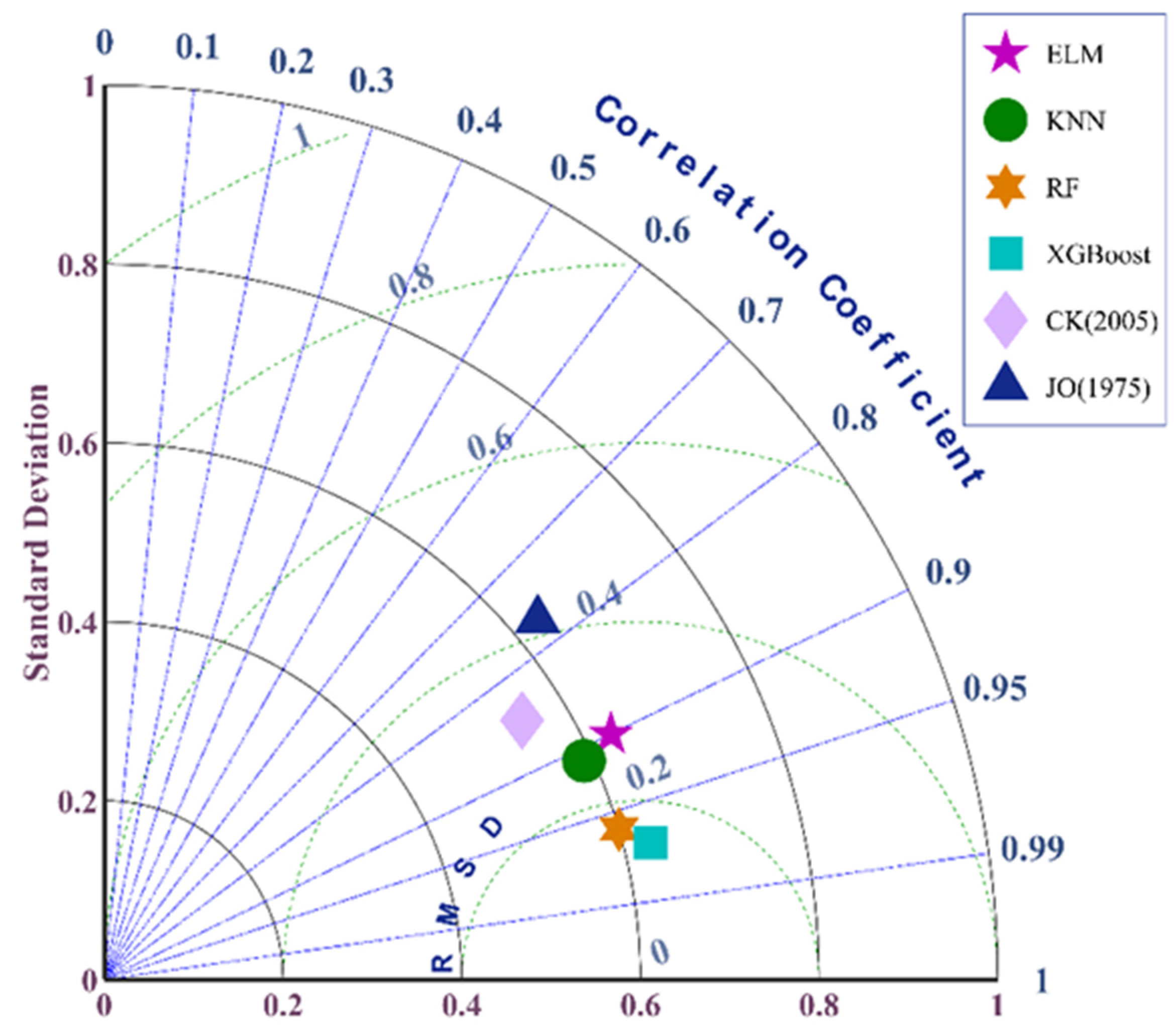
3.1. Optimal Model for Thermal Conductivity Simulations

To evaluate the generalization ability of the models, 70% of the thermal conductivity dataset was randomly selected for model simulation, and the remaining 30% was used for training. The hyperparameters for all models were determined using trial and error. The simulation and training results are presented in Figure 2 and Figure 3, respectively.
During training, all four machine learning models produced a good simulation performance, and the correlation coefficient (R) for the simulation and measured results were all above 0.91, with those for RF and XGBoost reaching 0.99. ELM had the weakest performance of the four models. The scatter plot of the training results shows that the measured and predicted results for RF and XGBoost were closely clustered around the 1:1 line. The fitted line for RF was below the 1:1 line with a lower slope, indicating that it underestimated the actual values, while the fitted line for XGBoost mostly overlapped the 1:1 line. In contrast, the scatter plots for the KNN and ELM methods were more scattered, with lower slopes and greater underestimation.
The simulation results for the four models using the test data were also generally reliable (Figure 3), with R > 0.9 and a ranking of XGBoost > RF > KNN > ELM. The accuracy of XGBoost therefore remained the highest, with the simulated scatter distribution closer to the 1:1 reference line. Overall, XGBoost and RF were the most reliable models for STC simulations.
Table 4 presents the performance evaluation data for the two traditional parametric models and the four machine learning model simulations. The simulation accuracy of the machine learning algorithms was generally higher than that of the traditional algorithms. XGBoost had a high R2 of 0.94 and an RMSE of 0.17, followed by the RF model (R2 = 0.93 and RSME = 0.18). The ELM had the lowest R2 of the four machine learning models (0.8), but it still outperformed the Côté and Konrad (2005) [36] and Johansen (1975) [34] models. The Adj. R2, R, MAE, and MSE metrics also suggested that XGBoost was the optimal simulation model. Figure 4 shows that XGBoost and RF were closer to the ideal reference point (RMSE = 0, R = 1, σ = 0.6), with lower σ values. In addition, for the prevalent underestimation problem (Figure 3), we made appropriate adjustments to some of the simulation parameters in practice, making the simulation results more reliable and close to the real situation.
In summary, among the six simulation methods considered in this study, the XGBoost model was identified as the ideal method for STC simulations on the Tibetan Plateau. The RF model was also found to be a reliable approach for this purpose. Compared with the machine learning models, the traditional parametric models were relatively weak in terms of their simulation accuracy and reliability. Therefore, the XGBoost model was employed for all subsequent STC simulations in the present study.

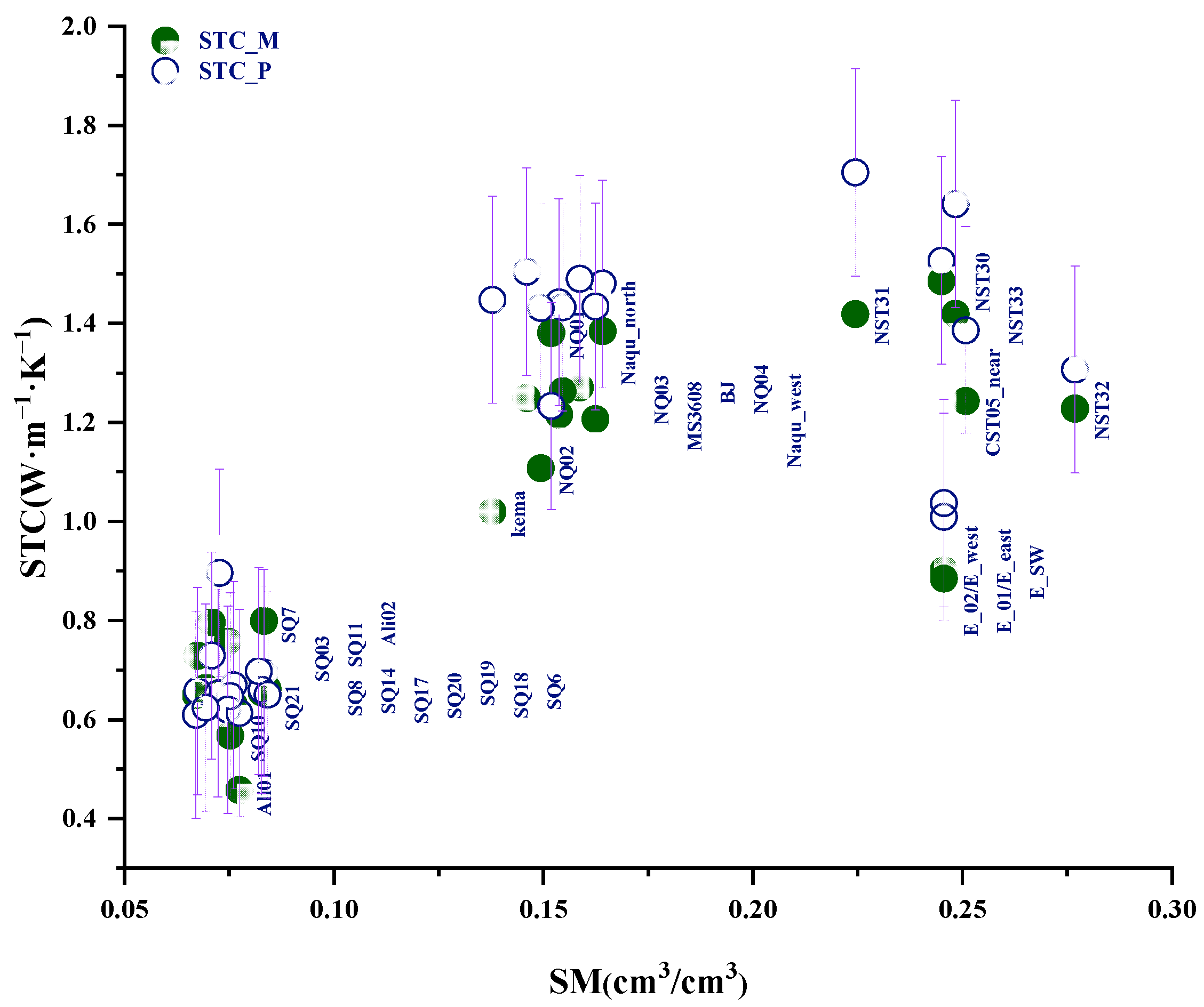
3.2. Verification of Product Reliability

Given the scarcity and limited spatial extent of the empirical thermal conductivity data for the plateau, this paper uses the in situ empirical measurements published by Zhao et al. (2018) [85] for the Maqu, Naqu, and Ngari regions in 2016. We used these data to validate the reliability of the 2015 products employed in our analysis. The locations of the field sites are shown in Figure 5. The Maqu sites include E02, E01, E_SW, CST05, NST30, NST31, NST32, and NST33; the Naqu sites include MS3608, BJ, Naqu_north, Naqu_west, NQ02, NQ03, NQ04, and NQ01; and the Ngari sites include Ali02, SQ17, SQ18, SQ21, SQ03, SQ10, SQ20, and SQ7. More details about each site can be found in the original paper [85].
Because soil moisture has a strong influence on the STC [11], the present study first analyzed the soil surface moisture data from the 2015 product and the in situ measurements from Zhao et al. (2018) [85] (Figure 6). The 2015 moisture data were in good agreement with the 2016 empirical measurements, with an absolute error of 0.015 cm3/cm3, a relative error of 11.4%, and a standard deviation of 0.03.
Based on these results and the assumption that the soil texture does not change dramatically in the short term, validation of the STC was subsequently conducted based on these two sets of data under different moisture conditions (Figure 7 and Figure 8).
The product data from August 2015 were in good agreement with the empirical STC measurements from August 2016, but the characteristics differed depending on the moisture content. At moisture levels lower than 0.1 cm3/cm3, the simulation results had very high accuracy. In particular, the absolute error for the predicted and measured results was 0.07 W m−1 K−1, the relative error was 11.5%, and the standard deviation was 0.07. However, for moisture levels of around 0.15 cm3/cm3, the difference between predicted and actual data was higher, with an absolute error of 0.23 W m−1 K−1, a relative error of 19.8%, and a standard deviation of 0.29. For moisture levels of around 0.25 cm3/cm3, the standard deviation for the simulation results was even larger (0.36), but the absolute and relative errors were lower, at 0.14 W m−1 K−1 and 12.5%, respectively. Given that the machine learning method used in the present study had a standard deviation of between 0.15 and 0.2 W m−1 K−1 (RSME = 0.17), the products employed in this study at different moisture contents can be considered relatively reliable.
It can also be observed from Figure 8 that the higher the soil moisture (i.e., the larger the circle), the higher the STC, highlighting the importance of soil moisture in predicting the STC. However, although the STC increased continuously with increasing total water content, the rate of this increase varied. In particular, for the thawing period in August, the STC initially increased linearly with higher moisture levels before gradually slowing down when the water content reached a certain level. The physical mechanism that explains this is that when the water content is lower than the maximum molecular water content, gases with lower thermal conductivity are present in the soil pores; as the water content increases, the gas content decreases, and the connection between the particle skeletons increases, reducing the contact thermal resistance between the particles. In addition, because the thermal conductivity of water is higher than that of gas, the STC increases rapidly [105,106]. When the water content in the soil is between the maximum molecular water content and the liquid limit water content, the thermal conductivity of the solid particles gradually becomes dominated by the water, and the water-induced bonding between the particle skeletons of the soil becomes secondary, thereby slowing the increase in the STC. When the water content is higher than the liquid limit, the water gradually begins to play a dominant role in the STC, which gradually approaches a fixed value. As such, the STC is related to both the water content and the nature and proportion of the solid soil particles [37,107].
Overall, STC is controlled by a combination of many internal and external factors, such as the mineral composition (especially the quartz content), salinity, soil freeze–thaw cycles, and the soil temperature; however, the soil moisture is its most critical factor. Given the shortcomings of machine learning, the lack of actual measurement data for STC, and the results of the validation process described above, it can be concluded that the proposed simulation methods, data products, and simulation results accurately reflect the general characteristics of the STC on the Tibetan Plateau. Although the present study sought to obtain highly accurate thermal conductivity products, there are still very few in situ observations available for the Tibetan Plateau, especially its vast western region, due to the harsh natural environment. Therefore, it was not possible to obtain a large amount of actual measured data to systematically evaluate of the model results for all of the data products used in this study. This remains an important consideration for future research.

3.3. Spatiotemporal Variation in the Thermal Conductivity by Month

In the present study, monthly data products from 2018 were used to analyze the monthly spatial distribution of the STC on the Tibetan Plateau to understand the trends in the STC at both monthly and macro scales.

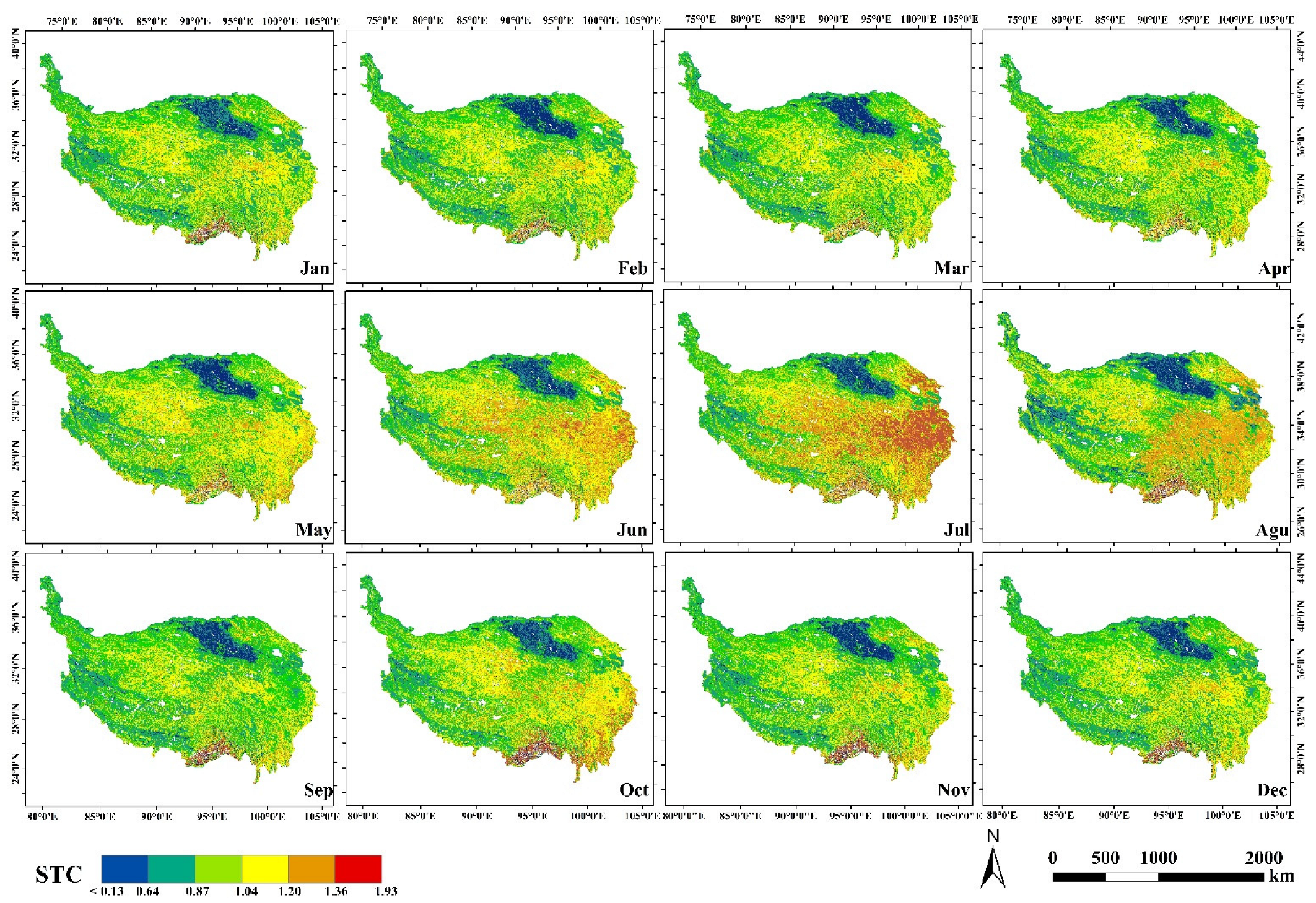
3.3.1. Temporal Variation in the STC

As shown in Figure 9, the monthly variation in the STC in 2018 on the Tibetan Plateau ranged from 0.13 to 1.93 W m−1 K−1 (±0.17). The highest STC values were 1.93 W m−1 K−1 and 1.91 W m−1 K−1 in June and July, respectively, followed by 1.87 W m−1 K−1 in September. The lowest STC values were observed in January and December (1.79 W m−1 K−1) and in February–April and October/November (1.85 W m−1 K−1). The highest values were found in July (1.1 W m−1 K−1), followed by June (1.05 W m−1 K−1), October (1.02 W m−1 K−1), and May (1.01 W m−1 K−1). The STC values for the remaining months were lower than 1 W m−1 K−1, with the lowest values in March, September, November, and December. Therefore, the maximum and average STC indicate that the conductivity was lower in months with colder temperatures.

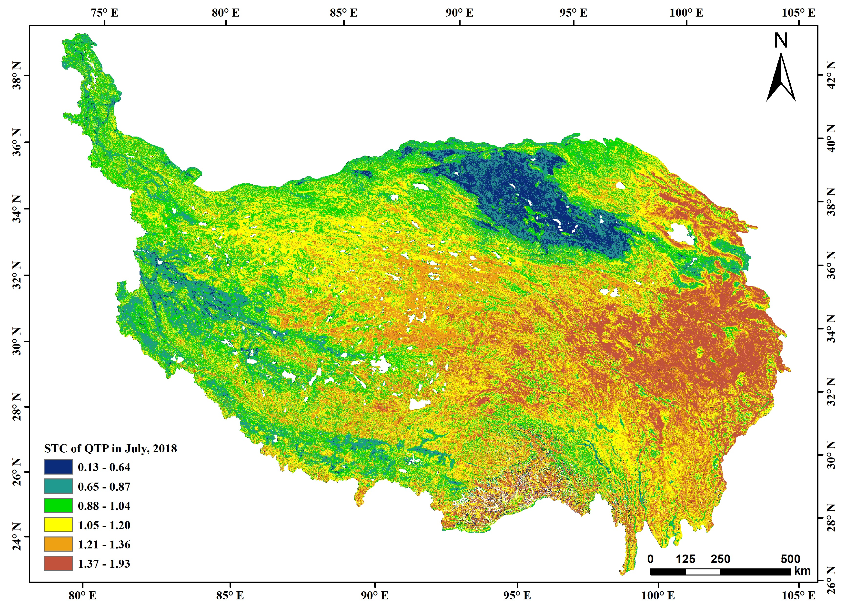
3.3.2. Spatial Variation in the STC in Different Months

Figure 10 shows that the spatial distribution of the STC in different months had significant seasonal differences. Throughout the whole plateau, the STC was high in the eastern and southeastern regions and low in the western and northwestern regions, with the lowest values observed in the Qaidam Basin and its northern area. In addition, the southern mountainous region had a high STC for a long time. In terms of monthly changes, from January to April, the STC gradually increased from the central to the eastern region and from the eastern fringe to the south. However, January to April is the freezing period, and the overall moisture levels in the active layer are low, so the overall STC was relatively low during this period. During the thawing period from May to August, the STC rapidly increased across the plateau, most obviously in the central and eastern regions, exceeding 1.36 W m−1 K−1 in July in several areas and reaching 1.93 W m−1 K−1 in some typical regions. In addition, in the northeastern part of the plateau north of Qinghai Lake, the STC in the Qilian Mountains increased dramatically during this period, with higher values than in other areas. However, a rapid decrease in the STC occurred in September in several areas, with a lower STC than in October in some areas. This was directly related to the soil surface moisture in September of that year. As the temperature decreases in October, soil freezing occurs in many parts of the plateau, and this ice–water phase change may occur in the shallow soil layer, leading to an increase in the STC. From October to December, the entire plateau enters the freezing period, and it was found that the STC as a whole decreased from east to west and from south to north (especially in the northwestern region), falling to below 1.2 W m−1 K−1 within a range of 0.64–1.20 W m−1 K−1 in most areas.
Overall, as shown by the monthly spatial distribution characteristics of the STC on the Tibetan Plateau in 2018, the STC was highest from May to August and lowest from January to April and from September to December, while the STC was generally higher in the central, central–eastern, and northeastern regions and lower in the Qaidam Basin and on the northern Tibetan Plateau.

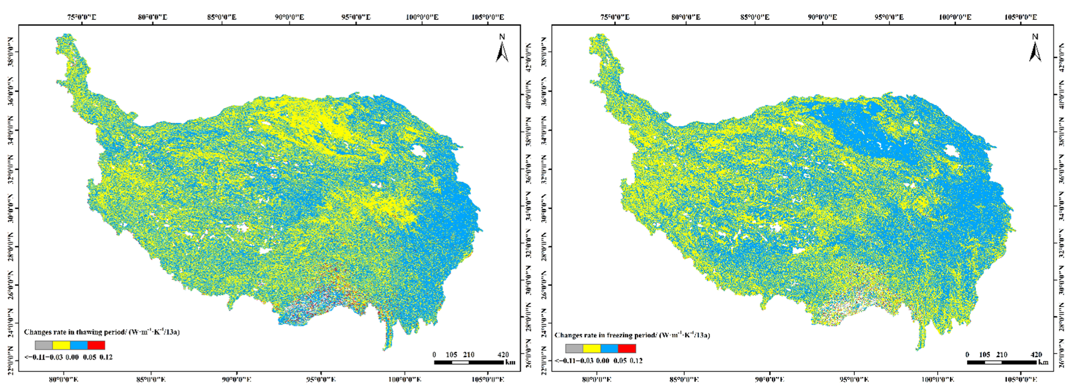
3.4. Spatiotemporal Variation in the Thermal Conductivity during the Freezing and Thawing Periods

In order to study the spatial distribution of STC during the thawing (May–September) and freezing (January–April and October–December) periods on the Tibetan Plateau and in the permafrost area, the mean soil moisture for the corresponding months during the two periods was calculated, based on which the STC for the two periods was calculated (Figure 11).
Across the entire Tibetan Plateau region, the STC during the thawing period (Figure 11a) was generally higher than that during the freezing period (Figure 11b), and the size of the area with an STC higher than 1.15 W m−1 K−1 during the thawing period was significantly larger than that during the freezing period.In terms of spatial distribution, the central–eastern region had a high STC during both periods, but the STC in the central part of the plateau, the northern Tibetan Plateau region, and the Qilian Mountains in the northern part of Qinghai Lake was higher during the thawing period, with some areas with a thermal conductivity above 2.0 W m−1 K−1, while the STC in the northwestern Kunlun Mountains region was also higher during the thawing period than during the freezing period as a whole.
For the permafrost zone of the Qinghai–Tibet Plateau, the STC pattern of high values in the east and low values in the west was similar to that of the plateau as a whole. In particular, during the thawing period (Figure 11c), the STC was higher in the central part of the permafrost, the central–eastern boundary area, and the eastern part of the Qilian Mountains permafrost zone in the northeast, with areas exceeding 1.32 W m−1 K−1, accounting for more than half of the entire permafrost zone. In the western and northwestern areas of the permafrost zone, the STC was above 0.98 W m−1 K−1, and only in some border areas in the north and southwest was the STC within the range of 0.78–0.98, with very few areas below 0.78 W m−1 K−1.
However, the spatial characteristics during the freezing period were quite different (Figure 11d). Specifically, the total STC in the eastern boundary of the permafrost during the freezing period was above 1.15 W m−1 K−1, while the STC in the rest of the western hinterland during the freezing period ranged from 0.78 to 1.15 W m−1 K−1, showing a clear pattern of spread from the center of the northern Tibetan Plateau to the west, northwest, and northeast. In the boundary zone of the permafrost in the western and southwestern parts of the plateau, the STC ranged from 0.47 to 0.98 W m−1 K−1, with very few areas exceeding 0.98 W m−1 K−1 (i.e., less than 1% of the total permafrost area). Therefore, in the permafrost area of the Tibetan Plateau, the STC is higher overall during the thawing period than during the freezing period, and higher in the eastern and southeastern regions than in the western and northwestern regions during these periods.

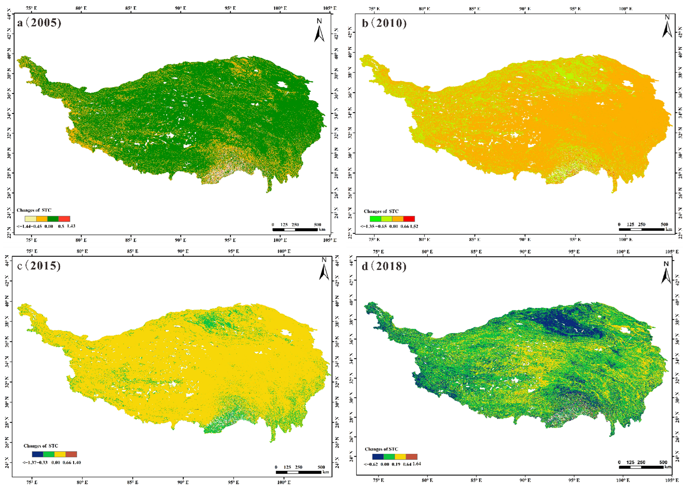
3.5. Interannual Variation in the Thermal Conductivity during the Freezing and Thawing Periods from 2005 to 2018

In order to macroscopically understand the long-term interannual spatiotemporal variation in the STC during the thawing and freezing periods on the Qinghai–Tibet Plateau and in the permafrost region, this study calculated the difference between the variation in the STC during the thawing and freezing periods for four periods (2005, 2010, 2015, and 2018; Figure 12, Figure 13 and Figure 14).
(1) Interannual changes in the spatial distribution of the thermal conductivity during the thawing and freezing periods
Throughout the study period from 2005 to 2018, the difference in the STC changes on the Tibetan Plateau clearly shows that the STC during the thawing period was higher than that during the freezing period as a whole (Figure 12a–d).
The range of the difference between the two periods in 2005 was between −1.44 and 1.43 W m−1 K−1, although in most areas, the difference was around 0–0.50 W m−1 K−1. The difference between the western border, the southern mountainous area, and some areas in the north range between −0.45 and 0 W m−1 K−1.
In 2010, the difference between the thawing and freezing period ranged between −1.35 and 1.52 W m−1 K−1, with most of the areas between −0.65 and 0.66 W m−1 K−1. Compared with 2005, the range of areas with a negative difference increased, especially in the western and northwestern regions, while the central and most of the eastern part maintained the trend of the STC being higher during the thawing period than during the freezing period.
In 2015, the difference between the thawing and freezing period decreased to within the range of −1.37 to 1.40 W m−1 K−1, and the negative range of their differences also decreased, gradually returning to southern and southeastern mountainous areas and the northern basin areas, with values between −0.33 and 0 W m−1 K−1. Some areas on the central plateau and the southern Tibetan Plateau in the west also had STC values below 0. With the exception of or these areas, the thermal conductivity of the thawing period was higher than that of the freezing period in most areas on the plateau, with a range concentrated between 0 and 0.66 W m−1 K−1.
In 2018, the range of STC differences between the thawing and freezing periods decreased compared with the previous three periods, ranging from −0.62 to 1.64 W m−1 K−1. There was an increase in the range of higher STC values during the thawing period than during the freezing period. The positive difference ranged from 0.19 to 0.64 W m−1 K−1 in the central and eastern regions of the plateau, and the difference was around 0 to 0.19 W m−1 K−1 in most of the remaining regions. In contrast, the areas with negative differences were still concentrated in the Qaidam Basin and its northern, southern mountainous, and southwestern marginal areas, with differences ranging from −0.62 to 0 W m−1 K−1.
(2) Spatial distribution of changes in the thermal conductivity during the thawing and freezing periods in the permafrost zone
The overall STC for the thawing period in the permafrost region of the Qinghai–Tibet Plateau from 2005 to 2018 was also higher than that for the freezing period, as indicated by the fact that the range of positive values for the difference between the two was significantly larger than the range of negative values.
In 2005, the difference between the thawing and freezing periods in the permafrost region ranged from −1.35 to 1.33 W m−1 K−1 (Figure 13a). The difference in the STC in the hinterland region had a range of 0–0.51 W m−1 K−1, while in the peripheral, western, and southern regions, the STC during the freezing period was higher than that during the thawing period, with a difference ranging from −0.45 to 0 W m−1 K−1. According to the in situ observations conducted by Li et al. (2019) at the Tanggula Station on the Qinghai–Tibet Plateau (E 91.86, N32.58, H 5100 m) from 2004 to 2008, the average annual thermal conductivity during the melting period was 1.56 W m−1 K−1, while the freezing thermal conductivity was 1.39 W m−1 K−1, and the difference between the two was about 0.18 W m−1 K−1. The difference in thermal conductivity between the melting period and the freezing period in 2005 was 0.26 W m−1 K−1, which is consistent with the conclusion of this study.
In 2010, the difference in the STC between the thawing and freezing periods in the permafrost region ranged from −1.27 to 1.52 W m−1 K−1 (Figure 13b). There was a gradual increase in the STC on the northern Tibet Plateau, and in the western region as a whole, the STC during the thawing period was higher than that during the freezing period, with values ranging from 0 to 0.18 W m−1 K−1. However, in some regions and permafrost boundary areas, the STC during the freezing period was higher than that during the thawing period (–1.27 to 0 W m−1 K−1). Toward the central and eastern border areas and the northeastern region, the STC during the thawing period was significantly higher than that during the freezing period, with values ranging from 0.18 to 0.61 W m−1 K−1. In the eastern and southeastern boundary areas of permafrost, the difference in the STC was 0.61–1.52 W m−1 K−1
In 2015, the difference between the thawing and freezing periods in the permafrost area ranged from −1.21 to 1.39 W m−1 K−1 (Figure 13c). Overall, the difference in STC in the permafrost hinterland area was positive, ranging from 0 to 1.39 W m−1 K−1, and from the central to the peripheral areas, the difference in the STC gradually decreased in the permafrost boundary area; the difference exhibited a decreasing trend, with values ranging from 0 to 0.24 W m−1 K−1. In the southern, southwestern, and northeastern marginal areas, the STC during the freezing period was higher than that during the thawing period, but the difference was not large (–0.04 to 0 W m−1 K−1).
In 2018, the difference between the thawing and freezing periods in the permafrost area ranged from −0.48 to 1.56 W m−1 K−1 (Figure 13d). Overall, the values were higher in the hinterland and central parts of the permafrost zone, with the difference ranging from 0 to 0.59 W m−1 K−1. However, in the southeastern, eastern, western, and northeastern border areas, the STC during the freezing period was higher than that during the thawing period, with a difference ranging from −0.48 to 0 W m−1 K−1.
(3) Annual variability and spatial distribution of differences in the thermal conductivity between the thawing and freezing periods from 2005 to 2018
The annual variation in the STC and its spatial distribution across the Tibetan Plateau during the 13-year period from 2005 to 2018 were investigated separately for the thawing and freezing periods (Figure 14).
During the thawing period, the variability in the STC on the plateau ranged from −0.11 to 0.12 W m−1 K−1 over the 13 years, with low variability in the east, high variability in the central and northern areas, and scattered variability in the west. The variability in the northeastern and eastern parts of the Tibetan Plateau was positive, ranging from 0 to 0.65 W m−1 K−1, while the STC in the southern mountainous areas ranged from 0.05 to 0.12 W m−1 K−1. In the northern, central–eastern, southern, and most of the western parts of the plateau, the annual variability in the STC was negative, ranging from −0.03 to 0 W m−1 K−1. During the freezing period, the variability in the eastern and northeastern parts of the plateau was positive, while the southern parts exhibited scattered high values ranging from 0.05 to 0.12 W m−1 K−1. In the hinterland of the plateau, both positive and negative values were present, and in the western region, the negative range in the STC variability was relatively wide. This interannual variation is consistent with the actual in situ observations. The 5-year observations (2004–2008) of Li et al. (2019) [11] on the soil thermal conductivity in the TGL permafrost region showed that the soil thermal conductivity of the site is gradually decreasing at a rate of 0.037 per year. This change may be related to the change in soil water content caused by the thickening of the layer.

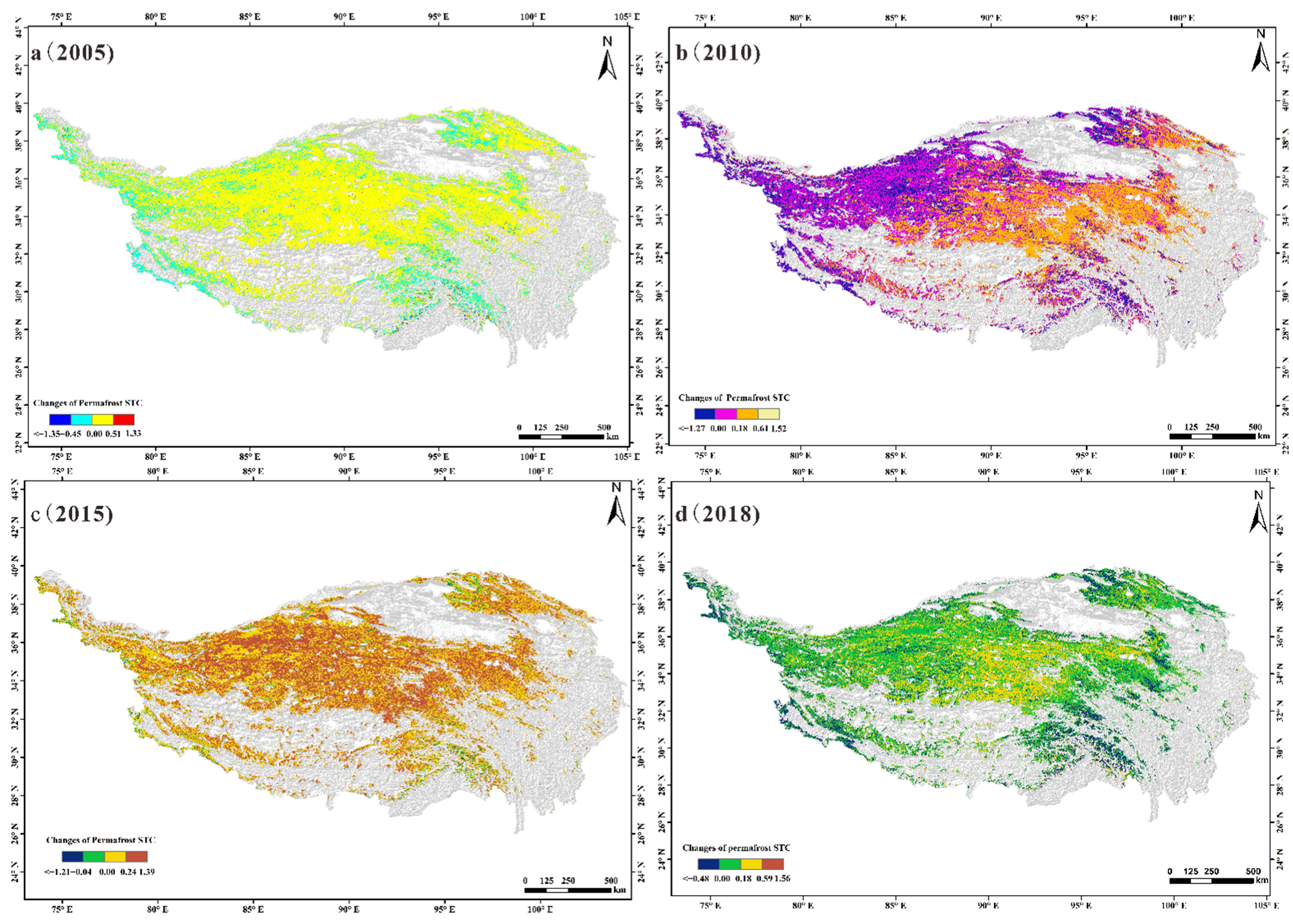
3.6. Distribution and Variation in the Thermal Conductivity of Different Underlying Surfaces in the Permafrost Zone

There are five main types of substratum in the permafrost area of the Qinghai–Tibet Plateau: bare land, alpine swamp meadow, alpine meadow, alpine steppe, and alpine desert. Of these, alpine meadow, alpine swamp meadow, alpine steppe, and alpine desert account for 48.59%, 4.18%, 27.69%, and 19.54% of the permafrost area, respectively [91]. Different substrates form an ecological equilibrium with the development of permafrost, and the growth and development of different types of vegetation are also key indicators of regional permafrost hydrothermal processes, climate, and precipitation [16,108]. In order to analyze the difference in the STC between the substrata, regional statistical analysis of the microscopic and macroscopic variation in the STC in the permafrost zone of the Qinghai–Tibet Plateau was conducted for the thawing and freezing periods based on the vegetation cover. The maximum, mean, variance, and variation range for the STC for the different vegetation types (Figure 15a) and the cumulative variation in the STC in different vegetation zones (Figure 15b) were determined.
The interannual variability of the STC for the 13 years from 2005 to 2018 (Figure 15a) shows that the maximum variability of the STC in the alpine meadow region was the largest during the thawing period, with the sum of the maximum and minimum values of the variability being 0.16 W m−1 K−1, followed by the alpine desert and alpine steppe, with 0.14 W m−1 K−1 and 0.13 W m−1 K−1, respectively. The variability in the STC in the alpine meadow region (0.21 W m−1 K−1) remained the largest during the freezing period, followed by the alpine desert (0.183 W m−1 K−1) and the alpine steppe (0.18 W m−1 K−1). The cumulative change in the STC over the 13-year period was negative during the thawing period for all vegetation types except alpine meadow and alpine steppe, indicating an overall decrease in the STC during the thawing period (Figure 15b). The magnitude of the cumulative value for the alpine desert and alpine swamp meadow was the highest, indicating a greater decrease in the STC in these substratum areas.
In contrast, the cumulative value for the STC in all vegetation areas was negative during the freezing period, indicating an overall decrease in the STC. For example, the negative cumulative value for the bare ground was −40.7 W m−1 K−1, which was the most variable type of the five sub-bedding areas, indicating that the STC of the bare ground during the freezing period was characterized by a negative increase during the 13 years from 2005 to 2018. The cumulative value of the STC in the alpine meadow and alpine steppe also showed a negative trend during this period.
Overall, from a microscopic perspective, the interannual variability in the STC showed that alpine meadows were the most sensitive to changes in the STC during the permafrost thawing and freezing periods. From a macroscopic perspective, the cumulative change in the interannual scale revealed that all vegetation types, except alpine meadows and alpine steppes, showed an overall decreasing trend in the STC over the 13-year period. In particular, bare land, alpine desert, and alpine swamp meadow areas were characterized by the most pronounced negative changes in the cumulative STC.

4. Discussion

4.1. Soil Moisture Is the Most Important Factor for the Spatial Difference of STC

4.1.1. Precipitation Determines the Monthly Variation of STC

The monthly STC data for 2018 show that STC is the highest from May to August and the lowest from January to April and September to December. This spatiotemporal variation in the monthly STC is, to some extent, the intuitive result of the combined influence of various factors, with soil moisture as the main controlling factor. In this regard, precipitation on the Tibetan Plateau was the main driving factor controlling the variation of the soil moisture levels at the soil surface and in the shallow layer (5 cm). In addition, the shallow soil layer, which is a sensitive zone for water–heat and energy interactions, is also strongly affected by temperature, surface stability, and solar radiation [109,110]. Differences in the effects of these factors between months, regions, and subsurface contexts are directly responsible for the variation in the monthly STC.

4.1.2. Spatial Differences in Moisture and Heat Determine the Spatial Distribution Pattern of STC during the Thawing and Freezing Periods

This regional variation in the STC on the Qinghai–Tibet Plateau and in the extensive permafrost areas during the thawing and freezing periods is affected by a number of factors, such as the climate, precipitation, topography, soil texture, and vegetation characteristics of the substratum [108,111]. In general, the thawing period is the period of the year during which the temperature is the highest and precipitation, under the influence of summer winds, is the greatest, so that the water in the soil is mainly in a liquid form and at higher levels [112], which directly leads to an increase in the STC across the plateau and permafrost areas. In contrast, the freezing period is characterized by a rapid decrease in the temperature (and solar radiation) and reduced precipitation, leading to a sharp decrease in liquid water content and an increase in the solid ice content. The spatial differences in moisture and heat between the two periods therefore determine the spatial distribution patterns of the STC.

4.1.3. Precipitation Causes a Gradual Decrease in the STC Difference between the Thawing and Freezing Periods in the Permafrost Zone

Comparing the spatial distribution of changes in the thermal conductivity during the thawing and freezing periods in the permafrost zone, we can find that the difference between the thawing and freezing periods in the permafrost region has been gradually decreasing, although it varies by region. In the hinterland of permafrost area, small changes in the western region and large changes in the eastern region were observed. In the eastern, southeastern, northwestern, and some small marginal areas in the west of the permafrost, the STC during the thawing period was lower than that during the freezing period; this trend is consistent with the characteristics of the whole plateau. The most important driver of these patterns was soil moisture, particularly the surface water and shallow soil moisture, which are controlled by precipitation [113,114]. In recent years, the permafrost region of the Tibetan Plateau has been characterized by warming and increased precipitation [108,115,116,117]. Except for the southeastern region, where annual precipitation has decreased significantly, precipitation has increased in most regions of the Tibetan Plateau, especially in the central and western areas and in the arid northwestern region. The annual precipitation in the arid northwestern permafrost region is the highest. In addition, the soil water levels in the permafrost region increased overall, with a slight decrease in areas with a high soil water content in the northeastern part of the Tibetan Plateau and an increase in the southwestern part of the Tibetan Plateau and most of the hinterland. These regional differences in precipitation and soil water content, as well as the processes associated with the ice–water phase change during the thawing and freezing periods, directly lead to interannual variation in the STC in the permafrost region during these two periods.

4.2. The Interannual Spatial Distribution Variation of STC from 2005 to 2018 Is Macroscopically Similar and Microscopically Homogeneous

The spatial patterns in the STC difference between the thawing and freezing periods over the years had similarities at the macroscopic scale. For example, in the northern and southern mountainous areas and around the basin of the whole plateau, the STC during the freezing period was more likely to be higher than that during the thawing period, possibly because the complex geomorphology, rich vegetation system, and higher soil moisture content at the beginning of the freezing period, as well as other favorable factors in these regions, influence the key physical processes associated with the change in the STC, resulting in the STC remaining high or decreasing more slowly during the freezing period. As a result, a negative difference between the freezing and thawing periods was observed in these areas.
In terms of microphysical mechanisms, the coarser soil texture and lower water-holding capacity of the soil on the Tibetan Plateau [118], coupled with its location in an arid and semiarid climate zone with low precipitation recharge, results in generally low water content in the surface soil. Regional precipitation recharge increases during the summer, resulting in relatively high soil water content during the thawing period, while at the beginning of freezing, precipitation on the plateau decreases significantly, and the surface soil water content becomes lower than a critical value, meaning that the thermal conductivity of the permafrost is lower than that of the thawing ground [11]. In contrast, in the mountainous regions and basins, where the soil texture is influenced by the topography, the moisture conditions are different from those of other regions, so the water content at the beginning of the freezing period may be above the critical level, resulting in a higher thermal conductivity during the freezing period than during the thawing period. However, this critical value may vary regionally due to factors such as the soil texture and composition [11,113,114,118]. Together, these microscopic mechanisms are responsible for the spatial distribution patterns of the STC on the Tibetan Plateau during the thawing and freezing periods.

4.3. The Reasons for the Differences in STC Variation Trends in Areas with Special Landforms during the Thawing and Freezing Periods Are Complex

The annual variability characteristics of the STC difference value during the thawing and freezing periods of the Qinghai–Tibet Plateau from 2005 to 2018 show that the STC of the whole plateau changed during the 13-year period, but the range of this change was limited. However, the spatial distribution showed significant differences. In areas with complex geomorphology such as basins and mountains, the change in the STC during the thawing and freezing periods exhibited different or even opposite trends. The reasons for these differences are complicated. In these areas, the weathering and cumulative precipitation of the soil are more intense, and the soil itself is subject to greater environmental influence, which may lead to changes in the soil texture and other factors in the soil that affect the STC, such as the levels of organic matter, quartz, gravel, and other components. Secondly, in these areas, local climatic zones are more likely to form, creating unique climatic phenomena such as extreme precipitation and drought that have a strong effects on the regional surface and subsurface shallow moisture. This results in different patterns in the STC in such areas with complex landforms.

5. Conclusions

In order to understand the spatiotemporal variation in the STC on the Tibetan Plateau and permafrost areas, this study established a thermal conductivity dataset consisting of 2972 measurements and employed an optimal machine learning method to investigate the monthly spatiotemporal variation in the STC during the freezing and thawing periods, the interannual variation in the STC during the freezing and thawing periods from 2005 to 2018, and the spatiotemporal variation in the STC on different substrates. The main conclusions of the present study are as follows.
First, by comparing the models proposed by Johansen (1975) and by Côté and Konrad (2005) and four machine learning models (ANN, KNN, ELM, and XGBoost), it was found that XGBoost is the optimal machine learning model for STC simulations, with the highest simulation accuracy. Using this method, STC data were obtained for the Qinghai–Tibet Plateau and permafrost. Data products for the STC of this region from 2005 to 2018 were obtained based on this method.
Second, the STC of the Qinghai–Tibet Plateau shows the following characteristics in terms of temporal variation and spatial distribution: (i) The results of the monthly STC analysis in 2018 showed that the STC was high from May to August and low from January to April and September to December. (ii) In terms of spatial differences, the STC was high in the central, central–eastern, and northeastern regions and low in the Qaidam Basin and the northern Tibetan Plateau. (iii) The mean STC during the thawing period was higher than that during the freezing period in the permafrost region as a whole, and the difference between the STC during the thawing and freezing periods gradually decreased in the eastern and southeastern regions relative to the western and northwestern regions. (iv) During the 13-year period from 2005 to 2018, the difference in the STC between the thawing and freezing periods in the permafrost region gradually decreased, and this change was smaller in the western part of the central region and larger in the eastern area; for the whole Tibetan Plateau, although the change in the STC was limited in its range, there were large differences in its spatial distribution, especially in the basin, mountainous areas, and other areas with complex landforms, where the trend of changes in STC during the thawing and freezing periods was different from that in other regions. (v) The STC in the alpine meadows was most sensitive to the changes in the thawing and freezing periods in the permafrost areas, while the STC in bare land, alpine desert, and alpine swamp meadow areas showed an overall decrease between 2005 and 2018.
Finally, the main reason for the spatiotemporal patterns in the STC on the Qinghai–Tibet Plateau and permafrost areas was the complex combination of climate, precipitation, topography, geomorphology, soil texture, and vegetation on the substrata, with precipitation-dominated differences in regional soil moisture being the key factor affecting the spatial distribution of the STC.
Outlook for this research: It should be pointed out that the thermal conductivity of soil varies greatly under different soil types and regional backgrounds. This study is the latest soil thermal conductivity data product in such a large-scale area of the Qinghai–Tibet Plateau. Although we evaluated the reliability of the data as much as possible from according to the aspects of data, methods, result verification, and comparative analysis, such unified data products still have inevitable limitations. For example, in terms of the base data, thousands of scales STC measurements were collected as far as possible in this study, but the number of these points distributed on the Tibetan Plateau still cannot meet the demand for more accurate simulations, and the representativeness of the points needs to be enhanced. In addition, the simulation is based on 10 influencing factors, and the problem of homogeneity and variability among different influencing factors needs to be further properly addressed. Finally, in the face of such a large area of the Tibetan Plateau, the use of a single model and data combination to carry out multiple types of STC simulations is bound to have large errors, especially the shallow depth of 5 cm carried out in this study is often affected by rainfall, snow, freeze-thaw and other types of influences, and the soil properties are easily affected, and the changes of related factors on STC deserve further attention. The mechanisms of unfrozen water and ice content, soil microstructure changes and other factors on STC under multiple freeze-thaw cycles also need to be further investigated. Therefore, this study concluded that carrying out the simulation combination of soil thermal conductivity calculation schemes according to different regional characteristics to meet the thermal conductivity modeling needs of different types of soil regions should be the focus of future attention in this field. The influence mechanism of various factors, including unfrozen water and ice content and soil microstructure changes under multiple freeze–thaw cycles, on soil thermal conductivity also needs to be further elucidated. The resolution of these problems will provide more reliable basic mechanistic support for more accurate simulation of thermal conductivity in permafrost regions.

Author Contributions

Conceptualization, W.L., R.L., T.W., and L.Z.; methodology, W.L., G.H., S.W., D.Z., and J.C.; software, D.W., X.Z., J.S., and J.M.; validation, X.S., X.W., Y.J., and J.Y.; formal analysis, W.L., Y.X., and R.L.; investigation, S.W., J.M., X.Z., J.C., and Y.Q.; resources, T.W., L.Z., X.W., J.S. and Y.Q.; data curation, W.L. and J.S.; writing—original draft preparation, W.L. and R.L.; funding acquisition, R.L., T.W., X.W., L.Z., and W.L. All authors have read and agreed to the published version of the manuscript.

Funding

This work was financially supported by the National Key Research and Development Program of China (No. 2020YFA0608502), the National Natural Science Foundation of China (42071093), the National Key Research and Development Program of China (No. 2020YFA0608500), the State Key Laboratory of Cryospheric Science (SKLCSZZ-2022), the National Natural Science Foundation of China (41961144021, 41941015, 32061143032, 41671070), the Youth Science and Technology Fund Plan of Gansu Province (21JR7RA063), and the Gansu Province Science and Technology Plan Project (22JR5RA061).

Data Availability Statement

Not applicable.

Acknowledgments

The dataset of soil moisture, soil texture, and permafrost distribution data was provided by the National Tibetan Plateau Data Center (http://data.tpdc.ac.cn (accessed on 20 November 2022)). Thanks to all the authors of the STC field study.

Conflicts of Interest

The authors declare no conflict of interest.

References

  1. Serikova, S.; Pokrovsky, O.S.; Laudon, H.; Krickov, I.V.; Lim, A.G.; Manasypov, R.M.; Karlsson, J. High Carbon Emissions from Thermokarst Lakes of Western Siberia. Nat. Commun. 2019, 10, 1552. [Google Scholar] [CrossRef] [Green Version]
  2. Song, C.; Wang, G.; Mao, T.; Dai, J.; Yang, D. Linkage between Permafrost Distribution and River Runoff Changes across the Arctic and the Tibetan Plateau. Sci. China Earth Sci. 2020, 63, 292–302. [Google Scholar] [CrossRef]
  3. You, Q.; Cai, Z.; Pepin, N.; Chen, D.; Ahrens, B.; Jiang, Z.; Wu, F.; Kang, S.; Zhang, R.; Wu, T. Warming Amplification over the Arctic Pole and Third Pole: Trends, Mechanisms and Consequences. Earth-Sci. Rev. 2021, 217, 103625. [Google Scholar] [CrossRef]
  4. Pörtner, H.-O.; Roberts, D.C.; Masson-Delmotte, V.; Zhai, P.; Tignor, M.; Poloczanska, E.; Mintenbeck, K.; Nicolai, M.; Okem, A.; Petzold, J. IPCC Special Report on the Ocean and Cryosphere in a Changing Climate; IPCC Intergovernmental Panel on Climate Change: Geneva, Switzerland, 2019; Volume 1. [Google Scholar]
  5. Bowen, J.C.; Ward, C.P.; Kling, G.W.; Cory, R.M. Arctic Amplification of Global Warming Strengthened by Sunlight Oxidation of Permafrost Carbon to CO2. Geophys. Res. Lett. 2020, 47, e2020GL087085. [Google Scholar] [CrossRef]
  6. Cheng, G.; Wu, T. Responses of Permafrost to Climate Change and Their Environmental Significance, Qinghai-Tibet Plateau. J. Geophys. Res. Earth Surf. 2007, 112, F02S03. [Google Scholar] [CrossRef] [Green Version]
  7. Miner, K.R.; Turetsky, M.R.; Malina, E.; Bartsch, A.; Tamminen, J.; McGuire, A.D.; Fix, A.; Sweeney, C.; Elder, C.D.; Miller, C.E. Permafrost Carbon Emissions in a Changing Arctic. Nat. Rev. Earth Environ. 2022, 3, 55–67. [Google Scholar] [CrossRef]
  8. Smith, S.L.; O’Neill, H.B.; Isaksen, K.; Noetzli, J.; Romanovsky, V.E. The Changing Thermal State of Permafrost. Nat. Rev. Earth Environ. 2022, 3, 10–23. [Google Scholar] [CrossRef]
  9. Hjort, J.; Streletskiy, D.; Doré, G.; Wu, Q.; Bjella, K.; Luoto, M. Impacts of Permafrost Degradation on Infrastructure. Nat. Rev. Earth Environ. 2022, 3, 24–38. [Google Scholar] [CrossRef]
  10. Ma, J.; Li, R.; Huang, Z.; Wu, T.; Wu, X.; Zhao, L.; Liu, H.; Hu, G.; Xiao, Y.; Du, Y. Evaluation and Spatio-Temporal Analysis of Surface Energy Flux in Permafrost Regions over the Qinghai-Tibet Plateau and Arctic Using CMIP6 Models. Int. J. Digit. Earth 2022, 15, 1948–1966. [Google Scholar] [CrossRef]
  11. Li, R.; Zhao, L.; Wu, T.; Wang, Q.; Ding, Y.; Yao, J.; Wu, X.; Hu, G.; Xiao, Y.; Du, Y. Soil Thermal Conductivity and Its Influencing Factors at the Tanggula Permafrost Region on the Qinghai–Tibet Plateau. Agric. For. Meteorol. 2019, 264, 235–246. [Google Scholar] [CrossRef]
  12. Lawrence, D.M.; Slater, A.G. Incorporating Organic Soil into a Global Climate Model. Clim. Dyn. 2008, 30, 145–160. [Google Scholar] [CrossRef]
  13. Tarnawski, V.R.; Leong, W.H. Advanced Geometric Mean Model for Predicting Thermal Conductivity of Unsaturated Soils. Int. J. Thermophys. 2016, 37, 18. [Google Scholar] [CrossRef]
  14. He, H.; He, D.; Jin, J.; Smits, K.M.; Dyck, M.; Wu, Q.; Si, B.; Lv, J. Room for Improvement: A Review and Evaluation of 24 Soil Thermal Conductivity Parameterization Schemes Commonly Used in Land-Surface, Hydrological, and Soil-Vegetation-Atmosphere Transfer Models. Earth-Sci. Rev. 2020, 211, 103419. [Google Scholar] [CrossRef]
  15. Comyn-Platt, E.; Hayman, G.; Huntingford, C.; Chadburn, S.E.; Burke, E.J.; Harper, A.B.; Collins, W.J.; Webber, C.P.; Powell, T.; Cox, P.M. Carbon Budgets for 1.5 and 2 C Targets Lowered by Natural Wetland and Permafrost Feedbacks. Nat. Geosci. 2018, 11, 568–573. [Google Scholar] [CrossRef] [Green Version]
  16. Niu, X.; Tang, J.; Chen, D.; Wang, S.; Ou, T. Elevation-dependent Warming over the Tibetan Plateau from an Ensemble of CORDEX-EA Regional Climate Simulations. J. Geophys. Res. Atmos. 2021, 126, e2020JD033997. [Google Scholar] [CrossRef]
  17. Slater, A.G.; Lawrence, D.M. Diagnosing Present and Future Permafrost from Climate Models. J. Clim. 2013, 26, 5608–5623. [Google Scholar] [CrossRef] [Green Version]
  18. Wang, C.; Wu, D.; Kong, Y.; Li, R.; Shi, H. Changes of Soil Thermal and Hydraulic Regimes in Northern Hemisphere Permafrost Regions over the 21st Century. Arct. Antarct. Alp. Res. 2017, 49, 305–319. [Google Scholar] [CrossRef] [Green Version]
  19. Wang, C.; Yang, K. A New Scheme for Considering Soil Water-heat Transport Coupling Based on Community Land Model: Model Description and Preliminary Validation. J. Adv. Model. Earth Syst. 2018, 10, 927–950. [Google Scholar] [CrossRef] [Green Version]
  20. Dai, Y.; Wei, N.; Yuan, H.; Zhang, S.; Shangguan, W.; Liu, S.; Lu, X.; Xin, Y. Evaluation of Soil Thermal Conductivity Schemes for Use in Land Surface Modeling. J. Adv. Model. Earth Syst. 2019, 11, 3454–3473. [Google Scholar] [CrossRef]
  21. Yang, S.; Li, R.; Wu, T.; Wu, X.; Zhao, L.; Hu, G.; Zhu, X.; Du, Y.; Xiao, Y.; Zhang, Y. Evaluation of Soil Thermal Conductivity Schemes Incorporated into CLM5. 0 in Permafrost Regions on the Tibetan Plateau. Geoderma 2021, 401, 115330. [Google Scholar] [CrossRef]
  22. Poutou, E.; Krinner, G.; Genthon, C.; de Noblet-Ducoudré, N. Role of Soil Freezing in Future Boreal Climate Change. Clim. Dyn. 2004, 23, 621–639. [Google Scholar] [CrossRef]
  23. Zhang, X.; Gao, Z.; Wei, D. The Sensitivity of Ground Surface Temperature Prediction to Soil Thermal Properties Using the Simple Biosphere Model (SiB2). Adv. Atmos. Sci. 2012, 29, 623–634. [Google Scholar] [CrossRef]
  24. Su, F.; Duan, X.; Chen, D.; Hao, Z.; Cuo, L. Evaluation of the Global Climate Models in the CMIP5 over the Tibetan Plateau. J. Clim. 2013, 26, 3187–3208. [Google Scholar] [CrossRef] [Green Version]
  25. Luo, S.; Fang, X.; Lyu, S.; Zhang, Y.; Chen, B. Improving CLM4. 5 Simulations of Land–Atmosphere Exchange during Freeze–Thaw Processes on the Tibetan Plateau. J. Meteorol. Res. 2017, 31, 916–930. [Google Scholar] [CrossRef]
  26. Zhu, D.; Ciais, P.; Krinner, G.; Maignan, F.; Jornet Puig, A.; Hugelius, G. Controls of Soil Organic Matter on Soil Thermal Dynamics in the Northern High Latitudes. Nat. Commun. 2019, 10, 3172. [Google Scholar] [CrossRef] [Green Version]
  27. Xiao, Y.; Zhao, L.; Dai, Y.; Li, R.; Pang, Q.; Yao, J. Representing Permafrost Properties in CoLM for the Qinghai–Xizang (Tibetan) Plateau. Cold Reg. Sci. Technol. 2013, 87, 68–77. [Google Scholar] [CrossRef]
  28. Hu, G.; Zhao, L.; Wu, X.; Li, R.; Wu, T.; Xie, C.; Pang, Q.; Xiao, Y.; Li, W.; Qiao, Y. Modeling Permafrost Properties in the Qinghai-Xizang (Tibet) Plateau. Sci. China Earth Sci. 2015, 58, 2309–2326. [Google Scholar] [CrossRef]
  29. Melton, J.R.; Arora, V.K.; Wisernig-Cojoc, E.; Seiler, C.; Fortier, M.; Chan, E.; Teckentrup, L. CLASSIC v1. 0: The Open-Source Community Successor to the Canadian Land Surface Scheme (CLASS) and the Canadian Terrestrial Ecosystem Model (CTEM)–Part 1: Model Framework and Site-Level Performance. Geosci. Model Dev. 2020, 13, 2825–2850. [Google Scholar] [CrossRef]
  30. Li, R.; Wu, T.H.; Zhao, L.; Xie, C.; Xiao, Y.; Hu, G.; Du, Y. Investigation on the Soil Thermal Conductivity of Different Land Surface Patterns in the Northern Qinghai-Tibetan Plateau, China. GEO Que. 2015, 548, 1–7. [Google Scholar]
  31. Zhang, N.; Wang, Z. Review of Soil Thermal Conductivity and Predictive Models. Int. J. Therm. Sci. 2017, 117, 172–183. [Google Scholar] [CrossRef]
  32. Malek, K.; Malek, K.; Khanmohammadi, F. Response of Soil Thermal Conductivity to Various Soil Properties. Int. Commun. Heat Mass Transf. 2021, 127, 105516. [Google Scholar] [CrossRef]
  33. De Vries, D.A. Thermal Properties of Soils. Phys. Plant Environ. 1963, 210–235. [Google Scholar]
  34. Johansen, O. Thermal Conductivity of Soils. Ph.D. Thesis, Trondheim University, Trondheim, Norway, 1975. [Google Scholar]
  35. Farouki, O.T. The Thermal Properties of Soils in Cold Regions. Cold Reg. Sci. Technol. 1981, 5, 67–75. [Google Scholar] [CrossRef]
  36. Côté, J.; Konrad, J.-M. A Generalized Thermal Conductivity Model for Soils and Construction Materials. Can. Geotech. J. 2005, 42, 443–458. [Google Scholar] [CrossRef]
  37. Lu, S.; Ren, T.; Gong, Y.; Horton, R. An Improved Model for Predicting Soil Thermal Conductivity from Water Content at Room Temperature. Soil Sci. Soc. Am. J. 2007, 71, 8–14. [Google Scholar] [CrossRef]
  38. He, H.; Zhao, Y.; Dyck, M.F.; Si, B.; Jin, H.; Lv, J.; Wang, J. A Modified Normalized Model for Predicting Effective Soil Thermal Conductivity. Acta Geotech. 2017, 12, 1281–1300. [Google Scholar] [CrossRef]
  39. He, H.; Flerchinger, G.N.; Kojima, Y.; He, D.; Hardegree, S.P.; Dyck, M.F.; Horton, R.; Wu, Q.; Si, B.; Lv, J. Evaluation of 14 Frozen Soil Thermal Conductivity Models with Observations and SHAW Model Simulations. Geoderma 2021, 403, 115207. [Google Scholar] [CrossRef]
  40. Du, Y.; Li, R.; Wu, T.; Yang, C.; Zhao, L.; Hu, G.; Xiao, Y.; Yang, S.; Ni, J.; Ma, J. A New Model for Predicting Soil Thermal Conductivity for Dry Soils. Int. J. Therm. Sci. 2022, 176, 107487. [Google Scholar] [CrossRef]
  41. Cuo, L.; Zhang, Y.; Bohn, T.J.; Zhao, L.; Li, J.; Liu, Q.; Zhou, B. Frozen Soil Degradation and Its Effects on Surface Hydrology in the Northern Tibetan Plateau. J. Geophys. Res. Atmos. 2015, 120, 8276–8298. [Google Scholar] [CrossRef] [Green Version]
  42. Wang, K.; Wang, P.; Liu, J.; Sparrow, M.; Haginoya, S.; Zhou, X. Variation of Surface Albedo and Soil Thermal Parameters with Soil Moisture Content at a Semi-Desert Site on the Western Tibetan Plateau. Bound.-Layer Meteorol. 2005, 116, 117–129. [Google Scholar] [CrossRef]
  43. Wang, D.; Wu, T.; Zhao, L.; Mu, C.; Li, R.; Wei, X.; Hu, G.; Zou, D.; Zhu, X.; Chen, J. A 1 Km Resolution Soil Organic Carbon Dataset for Frozen Ground in the Third Pole. Earth Syst. Sci. Data 2021, 13, 3453–3465. [Google Scholar] [CrossRef]
  44. Cao, X.; Tian, F.; Li, K.; Ni, J.; Yu, X.; Liu, L.; Wang, N. Lake Surface Sediment Pollen Dataset for the Alpine Meadow Vegetation Type from the Eastern Tibetan Plateau and Its Potential in Past Climate Reconstructions. Earth Syst. Sci. Data 2021, 13, 3525–3537. [Google Scholar] [CrossRef]
  45. Rao, P.; Wang, Y.; Wang, F.; Liu, Y.; Wang, X.; Wang, Z. Daily Soil Moisture Mapping at 1 Km Resolution Based on SMAP Data for Desertification Areas in Northern China. Earth Syst. Sci. Data 2022, 14, 3053–3073. [Google Scholar] [CrossRef]
  46. Zhang, Y.; Zhou, L.; Hu, Z.; Yu, Z.; Hao, S.; Lei, Z.; Xie, Y. Prediction of Layered Thermal Conductivity Using Artificial Neural Network in Order to Have Better Design of Ground Source Heat Pump System. Energies 2018, 11, 1896. [Google Scholar] [CrossRef] [Green Version]
  47. Rizvi, Z.H.; Husain, S.M.B.; Haider, H.; Wuttke, F. Effective Thermal Conductivity of Sands Estimated by Group Method of Data Handling (GMDH). Mater. Today Proc. 2020, 26, 2103–2107. [Google Scholar] [CrossRef]
  48. Rizvi, Z.H.; Zaidi, H.H.; Akhtar, S.J.; Sattari, A.S.; Wuttke, F. Soft and Hard Computation Methods for Estimation of the Effective Thermal Conductivity of Sands. Heat Mass Transf. 2020, 56, 1947–1959. [Google Scholar] [CrossRef]
  49. Zhang, T.; Wang, C.; Liu, S.; Zhang, N.; Zhang, T. Assessment of Soil Thermal Conduction Using Artificial Neural Network Models. Cold Reg. Sci. Technol. 2020, 169, 102907. [Google Scholar] [CrossRef]
  50. Wen, H.; Bi, J.; Guo, D. Calculation of the Thermal Conductivities of Fine-textured Soils Based on Multiple Linear Regression and Artificial Neural Networks. Eur. J. Soil Sci. 2020, 71, 568–579. [Google Scholar] [CrossRef]
  51. Fei, W.; Narsilio, G.A.; Disfani, M.M. Predicting Effective Thermal Conductivity in Sands Using an Artificial Neural Network with Multiscale Microstructural Parameters. Int. J. Heat Mass Transf. 2021, 170, 120997. [Google Scholar] [CrossRef]
  52. Bayat, H.; Ebrahimzadeh, G.; Mohanty, B.P. Investigating the Capability of Estimating Soil Thermal Conductivity Using Topographical Attributes for the Southern Great Plains, USA. Soil Tillage Res. 2021, 206, 104811. [Google Scholar] [CrossRef]
  53. Zhang, R.; Xue, X. A New Model for Prediction of Soil Thermal Conductivity. Int. Commun. Heat Mass Transf. 2021, 129, 105661. [Google Scholar] [CrossRef]
  54. Zhu, C.-Y.; He, Z.-Y.; Du, M.; Gong, L.; Wang, X. Predicting the Effective Thermal Conductivity of Unfrozen Soils with Various Water Contents Based on Artificial Neural Network. Nanotechnology 2021, 33, 065408. [Google Scholar] [CrossRef] [PubMed]
  55. Orakoglu Firat, M.E.; Atila, O. Investigation of the Thermal Conductivity of Soil Subjected to Freeze–Thaw Cycles Using the Artificial Neural Network Model. J. Therm. Anal. Calorim. 2022, 147, 8077–8093. [Google Scholar] [CrossRef]
  56. Li, K.-Q.; Kang, Q.; Nie, J.-Y.; Huang, X.-W. Artificial Neural Network for Predicting the Thermal Conductivity of Soils Based on a Systematic Database. Geothermics 2022, 103, 102416. [Google Scholar] [CrossRef]
  57. Chen, Y.; Yang, K.; Tang, W.; Qin, J.; Zhao, L. Parameterizing Soil Organic Carbon’s Impacts on Soil Porosity and Thermal Parameters for Eastern Tibet Grasslands. Sci. China Earth Sci. 2012, 55, 1001–1011. [Google Scholar] [CrossRef]
  58. Wang, X.; Yang, M.; Pang, G.; Wan, G.; Chen, X. Simulation and Improvement of Land Surface Processes in Nameqie, Central Tibetan Plateau, Using the Community Land Model (CLM3. 5). Environ. Earth Sci. 2015, 73, 7343–7357. [Google Scholar] [CrossRef]
  59. Hu, G.; Zhao, L.; Wu, X.; Li, R.; Wu, T.; Xie, C.; Pang, Q.; Zou, D. Comparison of the Thermal Conductivity Parameterizations for a Freeze-Thaw Algorithm with a Multi-Layered Soil in Permafrost Regions. Catena 2017, 156, 244–251. [Google Scholar] [CrossRef]
  60. Chen, S.X. Thermal Conductivity of Sands. Heat Mass Transf. 2008, 44, 1241–1246. [Google Scholar] [CrossRef]
  61. Hopmans, J.W.; Dane, J.H. Thermal Conductivity of Two Porous Media as a Function of Water Content, Temperature, and Density. Soil Sci. 1986, 142, 187–195. [Google Scholar] [CrossRef]
  62. Kasubuchi, T.; Momose, T.; Tsuchiya, F.; Tarnawski, V.R. Normalized Thermal Conductivity Model for Three Japanese Soils. Trans. Jpn. Soc. Irrig. Drain. Rural Eng. (Jpn.) 2007, 251, 53–57. [Google Scholar]
  63. McCombie, M.L.; Tarnawski, V.R.; Bovesecchi, G.; Coppa, P.; Leong, W.H. Thermal Conductivity of Pyroclastic Soil (Pozzolana) from the Environs of Rome. Int. J. Thermophys. 2017, 38, 21. [Google Scholar] [CrossRef]
  64. McInnes, K.J. Thermal Conductivities of Soils from Dryland Wheat Regions of Eastern Washington. Master’s Thesis, Washington State University, Spokane, DC, USA, 1981. [Google Scholar]
  65. Tarnawski, V.R.; McCombie, M.L.; Momose, T.; Sakaguchi, I.; Leong, W.H. Thermal Conductivity of Standard Sands. Part III. Full Range of Saturation. Int. J. Thermophys. 2013, 34, 1130–1147. [Google Scholar] [CrossRef]
  66. Tarnawski, V.R.; Momose, T.; McCombie, M.L.; Leong, W.H. Canadian Field Soils III. Thermal-Conductivity Data and Modeling. Int. J. Thermophys. 2015, 36, 119–156. [Google Scholar] [CrossRef]
  67. Zhao, Y.; Si, B.; Zhang, Z.; Li, M.; He, H.; Hill, R.L. A New Thermal Conductivity Model for Sandy and Peat Soils. Agric. For. Meteorol. 2019, 274, 95–105. [Google Scholar] [CrossRef]
  68. Barry-Macaulay, D.; Bouazza, A.; Wang, B.; Singh, R.M. Evaluation of Soil Thermal Conductivity Models. Can. Geotech. J. 2015, 52, 1892–1900. [Google Scholar] [CrossRef]
  69. Gori, F.; Corasaniti, S. New Model to Evaluate the Effective Thermal Conductivity of Three-Phase Soils. Int. Commun. Heat Mass Transf. 2013, 47, 1–6. [Google Scholar] [CrossRef]
  70. Hiraiwa, Y.; Kasubuchi, T. Temperature Dependence of Thermal Conductivity of Soil over a Wide Range of Temperature (5–75 °C). Eur. J. Soil Sci. 2000, 51, 211–218. [Google Scholar] [CrossRef]
  71. Kahr, G.; Müller-Vonmoos, M. Wärmeleitfähigkeit von Bentonit MX80 Und von Montigel Nach Der Heizdrahtmethode. Tech. Ber. NTB 82-06, Nagra, Hardstrasse 73, CH-5430 Wettingen, Schweiz. 1982. Available online: https://www.research-collection.ethz.ch/handle/20.500.11850/114577 (accessed on 22 November 2022).
  72. Tang, A.-M.; Cui, Y.-J.; Le, T.-T. A Study on the Thermal Conductivity of Compacted Bentonites. Appl. Clay Sci. 2008, 41, 181–189. [Google Scholar] [CrossRef] [Green Version]
  73. Lu, Y.; Yu, W.; Hu, D.; Liu, W. Experimental Study on the Thermal Conductivity of Aeolian Sand from the Tibetan Plateau. Cold Reg. Sci. Technol. 2018, 146, 1–8. [Google Scholar] [CrossRef]
  74. Nikolaev, I.V.; Leong, W.H.; Rosen, M.A. Experimental Investigation of Soil Thermal Conductivity over a Wide Temperature Range. Int. J. Thermophys. 2013, 34, 1110–1129. [Google Scholar] [CrossRef]
  75. Singh, D.N.; Devid, K. Generalized Relationships for Estimating Soil Thermal Resistivity. Exp. Therm. Fluid Sci. 2000, 22, 133–143. [Google Scholar] [CrossRef]
  76. Yamasaki, M.; Kawamura, Y. Thermal Diffusivity and Thermal Conductivity of Mg–Zn–Rare Earth Element Alloys with Long-Period Stacking Ordered Phase. Scr. Mater. 2009, 60, 264–267. [Google Scholar] [CrossRef]
  77. Zhang, N.; Yu, X.; Pradhan, A.; Puppala, A.J. A New Generalized Soil Thermal Conductivity Model for Sand–Kaolin Clay Mixtures Using Thermo-Time Domain Reflectometry Probe Test. Acta Geotech. 2017, 12, 739–752. [Google Scholar] [CrossRef]
  78. Mochizuki, H.; Mizoguchi, M.; Miyazaki, T. Effects of NaCl Concentration on the Thermal Conductivity of Sand and Glass Beads with Moisture Contents at Levels below Field Capacity. Soil Sci. Plant Nutr. 2008, 54, 829–838. [Google Scholar] [CrossRef]
  79. Campbell, G.S.; Jungbauer, J.D., Jr.; Bidlake, W.R.; Hungerford, R.D. Predicting the Effect of Temperature on Soil Thermal Conductivity. Soil Sci. 1994, 158, 307–313. [Google Scholar] [CrossRef]
  80. Tarnawski, V.R.; Tsuchiya, F.; Coppa, P.; Bovesecchi, G. Volcanic Soils: Inverse Modeling of Thermal Conductivity Data. Int. J. Thermophys. 2019, 40, 14. [Google Scholar] [CrossRef]
  81. Alrtimi, A.; Rouainia, M.; Haigh, S. Thermal Conductivity of a Sandy Soil. Appl. Therm. Eng. 2016, 106, 551–560. [Google Scholar] [CrossRef] [Green Version]
  82. Tokoro, T.; Ishikawa, T.; Shirai, S.; Nakamura, T. Estimation Methods for Thermal Conductivity of Sandy Soil with Electrical Characteristics. Soils Found. 2016, 56, 927–936. [Google Scholar] [CrossRef]
  83. Go, G.-H.; Lee, S.-R.; Kim, Y.-S.; Park, H.-K.; Yoon, S. A New Thermal Conductivity Estimation Model for Weathered Granite Soils in Korea. Geomech. Eng 2014, 6, 359–376. [Google Scholar] [CrossRef]
  84. Bristow, K.L. Measurement of Thermal Properties and Water Content of Unsaturated Sandy Soil Using Dual-Probe Heat-Pulse Probes. Agric. For. Meteorol. 1998, 89, 75–84. [Google Scholar] [CrossRef]
  85. Zhao, H.; Zeng, Y.; Lv, S.; Su, Z. Analysis of Soil Hydraulic and Thermal Properties for Land Surface Modeling over the Tibetan Plateau. Earth Syst. Sci. Data 2018, 10, 1031–1061. [Google Scholar] [CrossRef] [Green Version]
  86. Xu, X.; Zhang, W.; Fan, C.; Li, G. Effects of Temperature, Dry Density and Water Content on the Thermal Conductivity of Genhe Silty Clay. Results Phys. 2020, 16, 102830. [Google Scholar] [CrossRef]
  87. Bachmann, J.; Horton, R.; Van der Ploeg, R.R. Isothermal and Nonisothermal Evaporation from Four Sandy Soils of Different Water Repellency. Soil Sci. Soc. Am. J. 2001, 65, 1599–1607. [Google Scholar] [CrossRef]
  88. Al-Shammary, A.A.G.; Caballero-Calvo, A.; Jebur, H.A.; Khalbas, M.I.; Fernández-Gálvez, J. A Novel Heat-Pulse Probe for Measuring Soil Thermal Conductivity: Field Test under Different Tillage Practices. Comput. Electron. Agric. 2022, 202, 107414. [Google Scholar] [CrossRef]
  89. Kersten, M.S. Thermal Properties of Soils; University of Minnesota • Institute of Technology: Minneapolis, MN, USA, 1949. [Google Scholar]
  90. Zou, D.; Zhao, L.; Sheng, Y.; Chen, J.; Hu, G.; Wu, T.; Wu, J.; Xie, C.; Wu, X.; Pang, Q. A New Map of Permafrost Distribution on the Tibetan Plateau. Cryosphere 2017, 11, 2527–2542. [Google Scholar] [CrossRef] [Green Version]
  91. Wang, Z.; Wang, Q.; Zhao, L.; Wu, X.; Yue, G.; Zou, D.; Nan, Z.; Liu, G.; Pang, Q.; Fang, H. Mapping the Vegetation Distribution of the Permafrost Zone on the Qinghai-Tibet Plateau. J. Mt. Sci. 2016, 13, 1035–1046. [Google Scholar] [CrossRef]
  92. Hu, Z.; Chai, L.; Crow, W.T.; Liu, S.; Zhu, Z.; Zhou, J.; Qu, Y.; Liu, J.; Yang, S.; Lu, Z. Applying a Wavelet Transform Technique to Optimize General Fitting Models for SM Analysis: A Case Study in Downscaling over the Qinghai–Tibet Plateau. Remote Sens. 2022, 14, 3063. [Google Scholar] [CrossRef]
  93. Liu, F.; Wu, H.; Zhao, Y.; Li, D.; Yang, J.-L.; Song, X.; Shi, Z.; Zhu, A.-X.; Zhang, G.-L. Mapping High Resolution National Soil Information Grids of China. Sci. Bull. 2022, 67, 328–340. [Google Scholar] [CrossRef]
  94. Balland, V.; Arp, P.A. Modeling Soil Thermal Conductivities over a Wide Range of Conditions. J. Environ. Eng. Sci. 2005, 4, 549–558. [Google Scholar] [CrossRef]
  95. Pan, Y.; Lyu, S.; Li, S.; Gao, Y.; Meng, X.; Ao, Y.; Wang, S. Simulating the Role of Gravel in Freeze–Thaw Process on the Qinghai–Tibet Plateau. Theor. Appl. Climatol. 2017, 127, 1011–1022. [Google Scholar] [CrossRef]
  96. Zhao, T.; Liu, S.; Xu, J.; He, H.; Wang, D.; Horton, R.; Liu, G. Comparative Analysis of Seven Machine Learning Algorithms and Five Empirical Models to Estimate Soil Thermal Conductivity. Agric. For. Meteorol. 2022, 323, 109080. [Google Scholar] [CrossRef]
  97. Kang, J.; Yu, Z.; Wu, S.; Zhang, Y.; Gao, P. Feasibility Analysis of Extreme Learning Machine for Predicting Thermal Conductivity of Rocks. Environ. Earth Sci. 2021, 80, 455. [Google Scholar] [CrossRef]
  98. Kardani, N.; Bardhan, A.; Samui, P.; Nazem, M.; Zhou, A.; Armaghani, D.J. A Novel Technique Based on the Improved Firefly Algorithm Coupled with Extreme Learning Machine (ELM-IFF) for Predicting the Thermal Conductivity of Soil. Eng. Comput. 2022, 38, 3321–3340. [Google Scholar] [CrossRef]
  99. Kardani, N.; Bardhan, A.; Samui, P.; Nazem, M.; Asteris, P.G.; Zhou, A. Predicting the Thermal Conductivity of Soils Using Integrated Approach of ANN and PSO with Adaptive and Time-Varying Acceleration Coefficients. Int. J. Therm. Sci. 2022, 173, 107427. [Google Scholar] [CrossRef]
  100. Phan, T.N.; Kuch, V.; Lehnert, L.W. Land Cover Classification Using Google Earth Engine and Random Forest Classifier—The Role of Image Composition. Remote Sens. 2020, 12, 2411. [Google Scholar] [CrossRef]
  101. Magidi, J.; Nhamo, L.; Mpandeli, S.; Mabhaudhi, T. Application of the Random Forest Classifier to Map Irrigated Areas Using Google Earth Engine. Remote Sens. 2021, 13, 876. [Google Scholar] [CrossRef]
  102. Chen, T.; Guestrin, C. Xgboost: A Scalable Tree Boosting System. In Proceedings of the 22nd Acm Sigkdd International Conference on Knowledge Discovery and Data Mining, San Francisco, CA, USA, 13–17 August 2016; pp. 785–794. [Google Scholar]
  103. Dhaliwal, S.S.; Nahid, A.-A.; Abbas, R. Effective Intrusion Detection System Using XGBoost. Information 2018, 9, 149. [Google Scholar] [CrossRef] [Green Version]
  104. Qiu, Y.; Zhou, J.; Khandelwal, M.; Yang, H.; Yang, P.; Li, C. Performance Evaluation of Hybrid WOA-XGBoost, GWO-XGBoost and BO-XGBoost Models to Predict Blast-Induced Ground Vibration. Eng. Comput. 2022, 38, 4145–4162. [Google Scholar] [CrossRef]
  105. Jame, Y.-W.; Norum, D.I. Heat and Mass Transfer in a Freezing Unsaturated Porous Medium. Water Resour. Res. 1980, 16, 811–819. [Google Scholar] [CrossRef]
  106. Tao, Z.X.; Zhang, J.S. The Thermal Conductivity of Thawed and Frozen Soils with High Water (Ice) Content. J. Glaciol. Geocryol. 1983, 5, 75–80. [Google Scholar]
  107. Li, Y.; Shao, M.A.; Wang, W.Y.; Wang, Q.J.; Zhang, J.F.; Lai, J.B. Influence of Soil Textures on the Thermal Properties. Trans. Chin. Soc. Agric. Eng. 2003, 19, 62–65. [Google Scholar]
  108. Lin, Z.; Guojie, H.; Defu, Z.; Xiaodong, W.U.; Lu, M.A.; Zhe, S.U.N.; Liming, Y.; Huayun, Z.; Shibo, L.I.U. Permafrost Changes and Its Effects on Hydrological Processes on Qinghai-Tibet Plateau. Bull. Chin. Acad. Sci. 2019, 34, 1233–1246. (In Chinese) [Google Scholar]
  109. Ma, J.; Li, R.; Liu, H.; Huang, Z.; Wu, T.; Hu, G.; Xiao, Y.; Zhao, L.; Du, Y.; Yang, S. The Surface Energy Budget and Its Impact on the Freeze-Thaw Processes of Active Layer in Permafrost Regions of the Qinghai-Tibetan Plateau. Adv. Atmos. Sci. 2022, 39, 189–200. [Google Scholar] [CrossRef]
  110. Wang, S.; Li, R.; Wu, T.; Zhao, L.; Wu, X.; Hu, G.; Yao, J.; Ma, J.; Liu, W.; Jiao, Y. Evaluating the Impact of Soil Enthalpy upon the Thawing Process of the Active Layer in Permafrost Regions of the Qinghai–Tibet Plateau Using CLM5. 0. Remote Sens. 2022, 15, 249. [Google Scholar] [CrossRef]
  111. Gao, H.; Wang, J.; Yang, Y.; Pan, X.; Ding, Y.; Duan, Z. Permafrost Hydrology of the Qinghai-Tibet Plateau: A Review of Processes and Modeling. Front. Earth Sci. 2021, 8, 576838. [Google Scholar] [CrossRef]
  112. Li, H.; Liu, F.; Zhang, S.; Zhang, C.; Zhang, C.; Ma, W.; Luo, J. Drying–Wetting Changes of Surface Soil Moisture and the Influencing Factors in Permafrost Regions of the Qinghai-Tibet Plateau, China. Remote Sens. 2022, 14, 2915. [Google Scholar] [CrossRef]
  113. Xu, X.; Wang, J.-C.; Zhang, L.X. Permafrost Physics; Science Press: Beijing, China, 2001; Volume 351. [Google Scholar]
  114. Zhang, Y.; Ohata, T.; Kadota, T. Land-Surface Hydrological Processes in the Permafrost Region of the Eastern Tibetan Plateau. J. Hydrol. 2003, 283, 41–56. [Google Scholar] [CrossRef]
  115. Yao, T.; Xue, Y.; Chen, D.; Chen, F.; Thompson, L.; Cui, P.; Koike, T.; Lau, W.K.-M.; Lettenmaier, D.; Mosbrugger, V. Recent Third Pole’s Rapid Warming Accompanies Cryospheric Melt and Water Cycle Intensification and Interactions between Monsoon and Environment: Multidisciplinary Approach with Observations, Modeling, and Analysis. Bull. Am. Meteorol. Soc. 2019, 100, 423–444. [Google Scholar] [CrossRef]
  116. Yao, T.; Thompson, L.; Chen, D.; Piao, S. Reflections and Future Strategies for Third Pole Environment. Nat. Rev. Earth Environ. 2022, 3, 608–610. [Google Scholar] [CrossRef]
  117. Ma, Y.; Yao, T.; Zhong, L.; Wang, B.; Xu, X.; Hu, Z.; Ma, W.; Sun, F.; Han, C.; Li, M. Comprehensive Study of Energy and Water Exchange over the Tibetan Plateau: A Review and Perspective: From GAME/Tibet and CAMP/Tibet to TORP, TPEORP, and TPEITORP. Earth-Sci. Rev. 2023, 237, 104312. [Google Scholar] [CrossRef]
  118. Liu, Y.; Wu, X.; Wu, T.; Zhao, L.; Li, R.; Li, W.; Hu, G.; Zou, D.; Ni, J.; Du, Y. Soil Texture and Its Relationship with Environmental Factors on the Qinghai–Tibet Plateau. Remote Sens. 2022, 14, 3797. [Google Scholar] [CrossRef]
Figure 1. Correlation characteristics of 10 parameters and thermal conductivity (λ) in the dataset.
Remotesensing 15 01168 g001
Figure 2. Characteristics of training results of four models.
Remotesensing 15 01168 g002
Figure 3. Characteristics of test results of four models.
Remotesensing 15 01168 g003
Figure 4. Taylor diagram of test results for six models [34,36].
Remotesensing 15 01168 g004
Figure 5. Location of field verification points.
Remotesensing 15 01168 g005
Figure 6. Reliability evaluation of soil moisture data.
Remotesensing 15 01168 g006
Figure 7. Relationship between measured (STC_M) and simulated (STC_P) values of STC under different soil moisture conditions.
Remotesensing 15 01168 g007
Figure 8. Relation between measured (STC_M) and simulated (STC_P) results.
Remotesensing 15 01168 g008
Figure 9. Monthly values of STC on the Qinghai–Tibet Plateau in 2018.
Remotesensing 15 01168 g009
Figure 10. Monthly spatial distribution and variation characteristics of STC on the Qinghai–Tibet Plateau in 2018.
Remotesensing 15 01168 g010
Figure 11. Spatial distribution of STC during the thawing (a,c) and freezing periods (b,d) in the permafrost zone of the Qinghai–Tibet Plateau in 2018.
Remotesensing 15 01168 g011
Figure 12. Spatial distribution of interannual STC changes (value = STCthawing − STCfreezing) during the thawing (a,c) and freezing periods of the Qinghai–Tibet Plateau from 2005 to 2018 (b,d).
Remotesensing 15 01168 g012
Figure 13. Spatial distribution of STC difference value (=STCthawing − STCfreezing) during the thawing (a,c) and freezing periods (b,d) in the permafrost zone of the Qinghai–Tibet Plateau from 2005 to 2018.
Remotesensing 15 01168 g013
Figure 14. Annual variability characteristics of STC difference value during the thawing (left) and freezing (right) periods of the Qinghai–Tibet Plateau from 2005 to 2018.
Remotesensing 15 01168 g014
Figure 15. Interannual variation (a) and cumulative variation (b) of STC in different underlying surface types from 2005 to 2018.
Remotesensing 15 01168 g015
Table 1. The STC dataset used in this study.
Soil Species QuantityData VolumeλMean (W m−1 K−1)Data Sources
16801.42[60]
181.17[61]
3250.87[62]
191320.92[37]
2120.68[63]
5760.57[64]
6481.91[65]
402400.94[66]
8481.29[67]
6860.87[68]
322620.56[57]
160.89[69]
2180.55[70]
7330.74[71,72]
1561.58[73]
2231.19[74]
91310.59[75]
91050.46[76]
61001.34[77]
2210.71[78]
8730.68[79]
181.42[61]
10102.12[40]
222140.26[80]
1211.66[81]
3301.02[82]
2400.95[49]
12730.56[83]
1271.99[84]
56230.82[85]
191.36[86]
4721.57[87]
560.73[88]
182561.09[89]
2702972-[35]
Table 2. Eigenvalues of the STC dataset.
ParameterMeanStandard DeviationMinMax
Clay%0.1220.2020.0001.000
Silt%0.2850.2560.0000.900
Sand%0.5450.3300.0001.000
λs3.7161.5401.1178.030
Qtz0.4000.2690.0001.000
ρs2.6660.0602.1402.890
ρb1.3810.3020.2072.266
n0.4830.1150.1510.923
θw0.1720.1590.0000.846
Sr0.3300.2980.0001.000
λ0.8750.6640.0453.370
Table 3. Data products used in this study.
Data TypeProduct NamePrecisionYearsSources
Soil moistureDaily 0.01° × 0.01° Land Surface Soil Moisture Dataset of the Qinghai–Tibet Plateau (2005, 2010, 2015, 2017 and 2018)0.01° × 0.01°2005, 2010, 2015, 2018[92]
Soil textureDataset of digital soil mapping products for the Qinghai–Tibet Plateau (2015–2024)250 m
1 km
2015–2024[93]
Permafrost extentA new map of permafrost distribution on the Tibetan Plateau (2017)1 km2017[90]
Vegetation mapA new vegetation map for Qinghai–Tibet Plateau by integrated classification from multi-source data products (2020)250 m2020[91]
Table 4. Test performance of six models.
R2Adj. R2RRMSEMAEMSE
ELM0.800.650.900.300.210.09
KNN0.830.700.910.260.170.07
RF0.930.860.960.180.120.03
XGBoost0.940.880.970.170.110.03
CK (2005) [36] 0.710.510.850.360.240.13
JO (1975) [34]0.530.390.770.460.310.21
Disclaimer/Publisher’s Note: The statements, opinions and data contained in all publications are solely those of the individual author(s) and contributor(s) and not of MDPI and/or the editor(s). MDPI and/or the editor(s) disclaim responsibility for any injury to people or property resulting from any ideas, methods, instructions or products referred to in the content.

