Article

SAM-HIT: A Simulated Annealing Multispectral to Hyperspectral Imagery Data Transformation

1
Department of Geology, Faculty of Science, Aswan University, Aswan 81528, Egypt
2
Department of Petroleum and Geosystems Engineering, University of Texas at Austin, Austin, TX 78712, USA
3
Department of Geology, Faculty of Science, Benha University, Benha 13518, Egypt
4
Institute of Geosciences, University of Kiel, Ludewig-Meyn Str. 10, 24118 Kiel, Germany
*
Author to whom correspondence should be addressed.
Remote Sens. 2023, 15(4), 1154; https://doi.org/10.3390/rs15041154
Submission received: 25 January 2023 / Revised: 11 February 2023 / Accepted: 16 February 2023 / Published: 20 February 2023

Abstract

:
Space-borne hyperspectral imagery data are known for their high spectral resolution in a number of narrow wavelength intervals, which makes these data useful for mineral mapping. However, the available free-of-charge hyperspectral scenes cover only narrow and scattered geographic areas. In contrast, multispectral imagery scenes have a nearly complete spatial coverage and wider wavelength intervals. The low spectral resolution of the multispectral data, however, limits their efficiency in the mineral mapping of small geological massifs or hydrothermal alteration halos. The present contribution presents a new transformation tool (SAM-HIT) to simulate the hyperspectral sensor responses in unscanned areas based on partially overlapping hyperspectral and multispectral scenes. Simulation or prediction of the pseudohyperspectral data is here accomplished by using the simulated annealing linear optimization algorithm, which allows the lowest possible mismatch between the original and predicted data. The high visual and numerical correlation of the resultant data confirms the reliability of the newly adopted transformation. Further, the application of the SAM-HIT to a well-exposed part of the Egyptian basement complex with available hyperspectral data showed high concordance and nearly identical band signatures, opening a new outlook for mineral exploration in vast areas by a nearly automated cost-free means.

Graphical Abstract

1. Introduction

Satellite-based hyperspectral imagery data are widely used for mineral mapping due to their high spectral and spatial resolution. However, available hyperspectral imagery data cover only limited and very scattered geographic areas worldwide. In contrast, space-borne multispectral scenes are more widely available and have better spatial coverage, though with consistently lower spectral resolution. Therefore, efforts have been made to extrapolate hyperspectral data over unscanned areas by applying different methods [1,2]. Chen et al. used the pixel-mixing principle to create a new hyperspectral image while [3] being applied to the spectral unmixing approach. Both methods were based on fitting a linear relation between acquired space-borne data and laboratory and/or field samples’ spectral profiles. The focus of their work was mainly the identification of soils, vegetation, and water accumulations. Winter et al. [4] used inverse theory and employed a Hyperion band as a function of all the multispectral images. A multiple linear regression method was formulated and solved by least-squares optimization to predict suitable model parameters. A similar approach based on multiple linear regression, the PHITA algorithm, has been developed by [4], where the regression problem was solved using the Bayesian model averaging method to avoid overfitting [5]. The Bayesian model averaging technique uses generalized least-squares optimization to propose various solutions to the linear problem based on their posterior probabilities and whether or not the proposed model fits the linear relation. In the present study, we adopted the idea of multiple linear regression following [4,5] in a novel simulated annealing-based multispectral to hyperspectral imagery transformation (SAM-HIT) algorithm. The aim was to develop a fast simulated annealing algorithm to find the global optimum solution of the linear relation between the multispectral and hyperspectral data. Our proposed technique has been tested and validated through a well-studied and well-exposed area where different lithological units allow a knowledgeable and unbiased comparison.

2. Materials and Methods

2.1. Data and Method

For this study, we use seven Landsat 8 (L8) bands, with 30 m spatial resolution, and 155 Hyperion bands with the same spatial resolution (30 m/pixel), including bands 10–57 (447–926 nm), 81–97 (952–1115 nm), 101–119 (1154–1337 nm), 134–164 (1487–1791 nm), and 182–221 (1971–2365 nm). The only available Hyperion scene in the study area, downloaded from the USGS website, was acquired on 11 March 2003 while the L8 bands were acquired on 11 June 2022. The difference in acquisition dates has no significance on either the method or the result, as the mathematical approach, explained in the next paragraph, is fitted based on a linear relationship between both datasets. However, in case of landscape change or quarrying activities carried out between these two acquisition dates, the simulated Hyperion data that result from our transformation should represent the geological field status imaged on the date of L8 data acquisition. Although Hyperion bands are characterized by a low signal-to-noise ratio, they were spatially coherent and correlated well with the known geology, when tested for mineral mapping at Mount Fitton in South Australia [6]. Therefore, we use these 155 Hyperion bands as they are known for their stability and high quality [7]. The 155 Hyperion bands along with the L8 bands were used to train our algorithm to solve the multiple regression problem. Hyperspectral satellite data from the Italian satellite Prisma [8] were used to test the accuracy of our model visually. The satellite is owned and operated by ASI (Agenzia Spaziale Italiana). These genuine hyperspectral data are composed of 237 channels in total, with a 30 m spatial resolution. This includes 66 channel VIS/NIR bands with a spectral interval of 400–1010 nm, and 171 channel NIR/SWIR bands with a spectral interval of 920–2505 nm. A comprehensive description and user guide can be obtained through their website (https://www.eoportal.org/satellite-missions/Prisma-hyperspectral#Prisma (accessed on 30 August 2022)).
We assume that a Hyperion band is the product sum of several multispectral bands. This can be generalized by the simple linear formula,
Hi = Pi + Ci1B1 + Ci2B2 + … + CinBn
where Hi is the ith Hyperion band, Pi is the ith Hyperion band’s intercept (a constant value that equalizes the equation’s right part to its left part, e.g., the y-intercept of a line drawn in Cartesian coordinates), Ci1,Ci2, … and Cin are the coefficients of the (n) number of multispectral bands, and B1 and Bn are the (n) number of multispectral bands. Equation (1) can be expressed as
Hi = Gi X
where Hi is the matrix of the ith Hyperion band, X is a matrix of the multispectral bands, Gi is the Jacobian matrix (matrix of coefficients) of the ith Hyperion band, and * represents matrix multiplication. This formulates, for each band, a system of linear equations with many possible true solutions. However, one solution may fall in a local minimum, which causes overfitting. This can occur with inversion using the least-squares minimization method [5]. Hoang and Koike [4] used Bayesian model averaging (BMA) to overcome this problem in their PHITA algorithm. However, the PHITA algorithm still uses models derived from the standard least squares method, in which choosing the multispectral bands with high likelihood is not sufficient. Instead, we use the very fast simulated annealing algorithm, as it is a simpler approach that searches for the global optimum solution and overcomes the overfitting issue.
In 1953, [9] developed the simulated annealing (SA) method, also called Metropolis simulated annealing (MSA). It is based on the idea that, in metallurgy, the crystallization of a liquid alloy is governed by a cooling process. This is because cooling reduces the kinetic energy of atoms with high thermal mobility. In theory, a perfect crystal, with minimal overall atomic energy, is produced by infinitely slow cooling. On the other hand, a fast-cooling process freezes the solid in an imperfect or amorphous state. However, the atoms may achieve the optimal crystal structure through a slower cooling process by escaping from high-energy configurations through annealing. The perfect crystallization is analogous to the stabilization of the SAM-HIT procedure at the global optimum of the objective function while the amorphous state is analogous to the local minimum solution achieved by least-squares optimization.
The workflow of the conventional MSA algorithm starts by looping over an initial temperature or number of iteration steps where the assumption of a random model solution for the linear equation is proposed. Hence, initial values are given to Ci1 and Cin and Pi. The objective function, called energy in MSA, can then be calculated. The most widely used objective function is the L2 norm or the root mean squared error which describes the Euclidean distance between the real and simulated data:
E = 1 N i = 1 N ( d i ( o ) d i ( c ) ) 2
This energy function is minimized by modifying the model parameters and looping until a convergence is reached. The ith model parameter in the lth iteration step is modified according to
m i ( l + 1 ) = m i ( l ) + b
where b < bmax is a perturbation term and bmax is decreased as the iteration progress. After each iteration step, the energy function E(m) is calculated and compared with the previous one. The new model is either accepted or rejected according to the Metropolis criteria:
P ( Δ E , T ) = { 1 ,   i f   Δ E 0 e Δ E / T ,   o t h e r w i s e
The model is accepted when the value of energy function achieved by the new model is lower than that of the previous one. If it is greater, there is also a probability of acceptance depending on the energy differences and system temperature T. Therefore, the new model is accepted if P(ΔE, T) ≥ α, where α is a random number with uniform probability from the interval of 0 and 1. Otherwise, the model is rejected. By following these conditions, the model will avoid local minima. Cooling of the system, according to [10], follows Equation (6):
T ( l ) = T 0 ln ( l )   ( l > 1 )
where T0 is a specified initial temperature to reach the global optimum. However, this cooling schedule is time consuming. One of the most efficient attempts that shortens the CPU time is the modified SA algorithm, known as very fast simulated reannealing (VFSR) [11]. This algorithm considers different ranges of variation for each model parameter:
m i ( min )   m i ( l )   m i ( max )   ,
The ith model parameter is modified at iteration step (l + 1) as
m i ( l   + 1 ) =   m i ( l ) +   y i ( m i ( max ) m i ( min ) ) ,
where yi is a random number in the interval of −1 and 1. This number is generated from a nonuniform probability distribution function as follows:
y i = sign ( u 0.5 ) T i [ ( 1 + 1 T i ) | 2 u i 1 | 1 ] ,
where u is a random number in the range 0 and 1 with a uniform distribution, and the sign is randomly chosen (+/−). According to Equation (9), each model parameter is changed independently from the other parameters. The global optimum is then obtained when the cooling of each ith temperature follows
T i ( l ) = T 0 , i   e ( c l p )
where T0,i is the ith parameter’s initial temperature, ci is an arbitrarily chosen ith control parameter, and p is the number of model parameters. This does not limit the cooling schedule to a global system’s temperature. Instead, different temperatures are assigned to the model parameters, assuring the independent random modification of the model parameters. The VFSR algorithm accepts new models according to the Metropolis criteria with the exponential cooling schedule (Equation (10)) assuring much faster convergence to the global optimum.
In this study, our proposed SAM-HIT workflow (Figure 1) starts with looping over all Hyperion bands by constructing a data matrix with columns representing the Landsat images, and one column representing the Hyperion image to be fitted to the Landsat image dataset. A VFSR runs and finds the optimum solution of the linear equations for this Hyperion band. Eventually, a database comprising the optimal solutions for all the Hyperion bands is created. Having the database constructed, any Hyperion band can then be predicted over the entire area covered by the multispectral bands or any region of interest through simple matrix multiplication.
We have selected an area in the Central Eastern Desert of Egypt, the Barramiya-Um Salatit belt (Figure 2), to test our model since the area contains good exposures of different lithologies and varied metamorphic/deformational and intrusive structures [12].

2.2. Pre-Processing of Hyperion and L8 Images

The major problems with the Hyperion data include across-track illumination defects, stripes, reflectance defects, and brightness distortion [13]. Thus, the Hyperion bands were corrected for cross-track illumination defects by using the cross-track illumination correction (CTIC) module in the ENVI 5.3 software [14], which fits a polynomial function with a user-defined order and corrects the defect. These defects can be observed as a brightness gradient only in the first image, with the highest eigenvalue of the transformed minimum noise fraction (MNF) space. The correction was carried out using the CTIC module and then tested in a second MNF transformation. The correction and testing were repeated as a trial and error procedure until visual quality satisfaction was attained [13].
For destriping the Hyperion bands, the local destriping method was carried out in python. This is done by matching the mean and standard deviation of each column with the full band [15] as in the following equation:
v ¯ ijk   = ( v ijk μ jk ) σ k σ jk + μ k
where for a band with band number k, the new pixel value v ¯ ijk   at the ith row and jth column is a function of the original pixel value   v ijk , the arithmetic mean and standard deviation of the jth column μ jk , and σ jk , respectively, as well as the arithmetic mean and standard deviation of the kth band μ k and σ k .
The radiometric calibration was then accomplished as a prerequisite for the proceeding atmospheric correction using the FLAASH module, which delivers more reliable results than other atmospheric correction models [16].
ASI provides the Prisma data at different levels of processing. We used the L2 level (geolocated and geocoded atmospherically corrected).

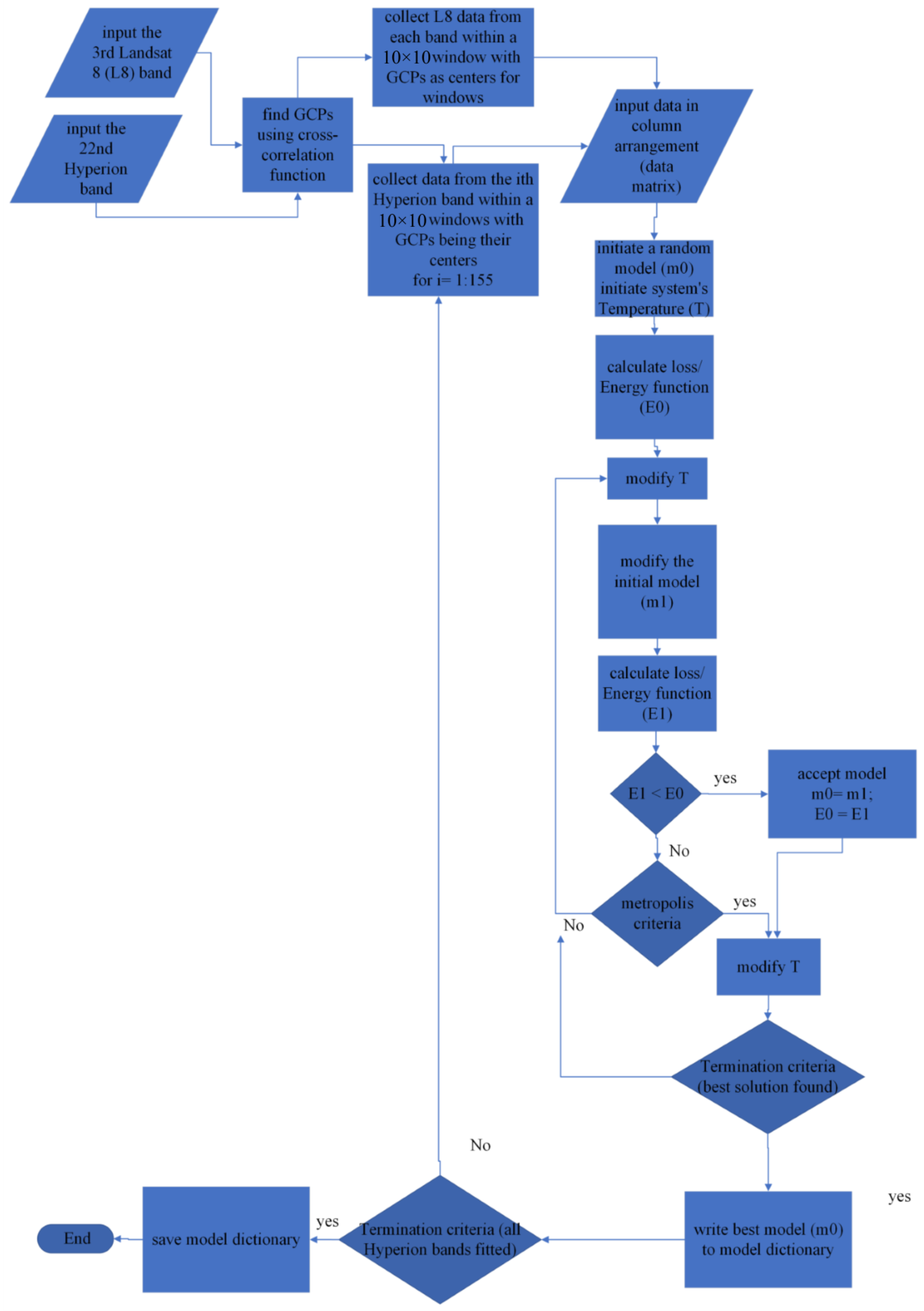
2.3. SAM-HIT Implementation

Predicting the hyperspectral images by this algorithm is accomplished through four steps, following the workflow of the SAM-HIT algorithm shown in Figure 1: collecting accurate data, finding the best solution, constructing the dictionary of models, and predicting the required bands in the region of interest. For collecting data, both L8 and Hyperion bands were normalized to have a common data scale (16-bit unsigned integer data type). The routine workflow in collecting these data incorporates image registration using ground control points (GCP), then warping the hyperspectral image to fit the L8 intersection. However, this process leads to the interpolation as well as warping of hundreds of thousands of pixels using a limited number of GCPs. In our workflow, we preferred to decrease the uncertainty of the data used as inputs to our model. We, therefore, use the cross-correlation function, Equation (12), for a hyperspectral band H and a multispectral band E, to define adequate GCPs that are distributed all over the Hyperion band and represent almost all the existing color tones. Consequently, we use these GCPs as centers for the 10 by 10 window within which the data is collected.
G [ i , j ] = u = k k v = l l H [ u , v ] E [ i + u , j + v ]
Figure 3 shows the uncertainty of warped data compared with a 10 by 10 window sampler as well as data representing only the GCPs. It is clear that the warped data, even after Gaussian filtering to remove outliers, can easily cause uncertain data models. The data collected for the 22nd Hyperion band versus the L8 third band is shown in Figure 4, revealing an excellent correlation of the data collected using a 10 by 10 window sampler around each GCP. The very fast simulated annealing algorithm is therefore used to solve the linear equation defined in Equation (2). This is accomplished by first assuming an initial random solution and modifying its parameters according to Equation (8), where the parameters were allowed to be within a range of (0–1), as shown in Equation (7). However, it is also possible to modify the parameters’ range to a wider interval. Hence, the best solution is that which achieves the global minimum of the objective/energy function defined in Equation (3), as the root mean squared error between original and predicted images. Eventually, the cooling schedule follows Equation (10), and the full process is accomplished through 20,000 iteration steps. This results in the best model parameters, which are then saved to the model dictionary. While the seeking process progresses, a single L8 band, or several bands, may be neglected by assigning a model parameter near or equal to zero. This is what the PHITA algorithm tests. If the SAM-HIT algorithm did not accept this solution, then it cannot be the global optimal. The SAM-HIT algorithm is therefore a more general workflow that tests an enormous number of solutions to find the global optimum (20,000 solutions in this case). Table 1 shows the sensitivity of the SAM-HIT algorithm in adequate band selection for the global optimum model where some bands were given approximately very low weight while others were given a significant weight to keep the correlation coefficient between the original and predicted result in a perfect fit. The next step encompasses predicting the hyperspectral image which covers the same spatial coverage as the multispectral one. This step is carried out through simple multiplication using the full scene of the L8 bands and their corresponding coefficients according to Equation (1).
Having the SAM-HIT workflow completed, 155 hyperspectral bands, as per our initial choice for healthy bands, are obtained with the advantage of covering the spatial extent of L8 bands.

3. Results

The method used a band-by-band comparison based on the visual similarity of original versus predicted Hyperion bands, along with their histograms. A comparison between both the original and the predicted Hyperion band 45 (wavelength = 803.3 nm) is shown in Figure 5, where the spatial variation and characteristics have been successfully captured, as indicated by their histograms. These show the predicted values with a slight shift to the white region, though having a similar distribution. This is supported by the composite band representations in Figure 6. Moreover, it is also seen in Figure 7 that the minimum, mean, maximum, and quartiles of the predicted Hyperion bands match very well with those of the original data.
For a full-data-based comparison, principal component analysis was used to reduce the dimensionality of the original and predicted data. We found that the first three principal components represent more than 99% of the information given by the 155 Hyperion bands (Table 2). The first three components for the original and predicted data were combined in an RGB composite for a visual similarity check. Figure 8 reveals that the predicted bands match very well with the original ones.
For a final stage of validation, the predicted Hyperion bands were compared with the original hyperspectral bands that were not used while training our model. Since Prisma data is slightly different from the Hyperion bands, we compared the predicted Hyperion bands and Prisma bands based on RGB composites for similar wavelengths. In Figure 9 and Figure 10, composite RGB of the predicted Hyperion bands (R = 83, G = 35, B = 16) and (R = 146, G = 30, B = 13) are superimposed with a similar wavelength RGB composite of two Prisma datasets along with the same RGB composite of the original Hyperion bands. It is clear that the predicted Hyperion bands have successfully captured the spatial and radiometric characteristics of the original Hyperion and Prisma datasets.

4. Discussion

In this work, we employed a very fast simulated annealing algorithm to obtain the optimal solution for the multiregression transformation of multispectral bands (Landsat 8) into hyperspectral ones (Hyperion). The method is a global optimization method that can avoid the local optimal solution that affects many of the other previously published transformations (e.g., [4,5]). The input was imported from a sampling window covering all or most of the colors through image registration based on the cross-correlation function. The advantage of this data collection is the way it overcomes the unwanted data interpolation resulting from the warping of the hyperspectral images on multispectral ones.
The resultant hyperspectral data were visually and statistically tested and validated. Statistically (Figure 5 and Figure 7), the predicted data showed excellent correlation, with almost identical minima, maxima, average, and standard deviation values for the different bands. Nonetheless, the resultant hyperspectral images have less color saturation (Figure 5), which normally has no significant effect on the lithological discrimination. The predicted pseudohyperspectral bands were then tested against the original ones in grayscale band by band (Figure 5), and true and false RGB composites (Figure 6), which show very good correlations.
The principal component analysis was also tested on both the original and predicted hyperspectral data to test the global similarity between the original and predicted data. A red-green-blue (RGB) combination of the principal components of the original and predicted data shows excellent similarity (Figure 8). Furthermore, we have validated our model’s result using the Prisma hyperspectral dataset, which was not used to train our model. The result (Figure 9 and Figure 10) demonstrates the efficiency of the transformation presented here to predict unavailable hyperspectral data.
Moreover, as an additional validation step, the Abrams ratios [17] were processed using the equivalent bands for Landsat-8 (6/7, 5/6, and 4/2), the original Hyperion data, the predicted hyperspectral data (142/201, 53/142, and 30/15), and the Prisma data (72/129, 50/72, and 34/12). The spectral response curves of rock-forming minerals show diagnostic absorption features throughout the visible near infrared and shortwave infrared wavelength ranges (0.325 to 2.5 µm). The main processes responsible for such features are electronic transition, vibrational overtones, charge transfer, and conduction [18,19]. Based on vibrational transitions of Al-OH, Fe-OH, and Mg-OH, hydroxyl-bearing silicate minerals (e.g., muscovite, kaolinite, epidote, chlorite, antigorite, chrysotile, and talc) exhibit important absorption features near 2.20 µm and 2.32 µm SWIR wavelengths [20]. Carbonate minerals (e.g., dolomite and calcite) show the most distinctive absorption features at 2.33 µm and 2.35 µm SWIR wavelengths [21]. In the TIR region, the silicate minerals (e.g., feldspars, mica, amphibole, pyroxene, and olivine) display intense absorption features in the wavelength range of 8.5 to 12 µm [22].
The Barramiya–Um Salatit district (Figure 11) has exposures of variably carbonatized and silicified ophiolitic mélange blocks that are tectonically incorporated in variably deformed metasedimentary and volcano–sedimentary matrices. These rocks are intruded by a wide spectrum of granitic intrusions ranging in composition from quartz-diorite, granodiorite-tonalite, to leucogranite [12]. The greyscale band ratio (6/7), (142/201), and (72/129) images clearly discriminate the variably talc-carbonatized/silicified zones as bright to white image signatures. Also, the Fe-rich silicate bearing zones appear with bright image signatures on the greyscale band ratio (vnir 5/vnir 6), (vnir 53/swir 142), and (vnir 50/swir 72) images (Figure 12 and Figure 13). Based on the RGB combination of band ratios (R: 6/7, G: 5/6, and B: 4/2) of Landsat 8, (R: 142/201, G: 53/142, and B: 30/15) of Hyperion and (R: swir 72/swir 129, G: vnir 50/swir 72, and B: vnir 34/vnir 12) of the Prisma, the false color band ratio composites (FCC) are best to discriminate the variably talc-carbonatized and silicified ophiolitic rocks with yellow, rose and orange image signatures. The quartz-diorite, granodiorite–tonalite and leucocratic granitoids appear with bluish-green, greenish, and pinkish colors, respectively (Figure 13C and Figure 14). On the other hand, the gabbroic rocks and basic metavolcanics exhibit dark green image signatures, the intermediate to acidic metavolcanics appear with brown and dark red colors, while the molasse-type sediments and metasediments exhibit light green and lemon greenish image signatures, respectively. It is clear that the image signatures of lithologies on the grayscale and FCC band ratio images of both the original and predicted hyperspectral data are correlated and more enhanced than those of multispectral Landsat-8 data. Figure 15 shows the Abrams ratio for the original Hyperion, Prisma, predicted Hyperion, and Landsat 8. The color grades shown in the original Hyperion and Prisma are closer to those of the predicted Hyperion than the Landsat 8 as the predicted Hyperion and Prisma have closer wavelengths while there are spectral gaps between them and the Landsat 8. This illustrates the success of our transformation to model hyperspectral rather than multispectral sources.

5. Conclusions

In geological studies, the high spectral resolution of hyperspectral data can be employed for a sharper discrimination of lithologies and hydrothermal alteration types. Our model demonstrates that predicting hyperspectral data for any geographic region of interest is possible. The simulated annealing algorithm was used here as a global optimization technique to train and define a global optimum model that can efficiently extrapolate hyperspectral data in areas not covered by Hyperion scenes. As a prerequisite, the area must have multispectral data, e.g., Landsat 8 or ASTER. The numerical and visual comparison between our model’s results and the original data confirm the accuracy of our newly designed transformation as an efficient means and a reliable simulator of the Hyperion sensor responses to different lithologies and offer a new means of advanced space-borne-based mapping.
Validation of the SAM-HIT transformation technique returns excellent results and shows that our model’s behavior is not affected by overfitting. Our transformation can be accomplished using any kind of multispectral dataset to predict hyperspectral data. We, therefore, recommend using available hyperspectral scenes to decrease the uncertainty of the generated hyperspectral dataset. However, a more independent method requires finding the best global optimum model and designing an automatic global hyperspectral simulator, which will be the subject of an outlook study. Codes, analyses, and visualizations have been written in Python as well as ArcGIS and Envi software. The newly designed SAM-HIT code will be published as an open-source python package in a future publication.

Author Contributions

Conceptualization, B.Z. and A.M.; methodology, A.M.; software, A.E. and A.M.; validation, A.M., A.E. and B.Z.; formal analysis, B.Z. and A.E.; investigation, A.M.; resources, A.E.; data curation, A.M.; writing—original draft preparation, A.M.; writing—review and editing, B.Z. and A.E.; visualization, A.M.; supervision, B.Z.; project administration, B.Z. All authors have read and agreed to the published version of the manuscript.

Funding

This research received no external funding.

Data Availability Statement

Not applicable.

Acknowledgments

The authors thank the USGS for the public use of the different multispectral datasets. We acknowledge the granted access to the PRISMA data (a hyperspectral sensor with a medium resolution), acquired by a mission funded by Italian Space Agency (ASI). Indeed, the availability of the multispectral and hyperspectral data promoted this study. Hugh Daigle, associate professor at University of Texas, Austin, is thanked for his help with the proofreading of the early manuscript. Two journal anonymous reviewers are thanked for their useful comments and suggestions.

Conflicts of Interest

The authors declare no conflict of interest.

References

  1. Chen, F.; Niu, Z.; Sun, G.; Wang, C.; Teng, J. Using Low-spectral-resolution Images to Acquire Simulated Hyperspectral Images. Int. J. Remote Sens. 2008, 29, 2963–2980. [Google Scholar] [CrossRef]
  2. Berezowski, T.; Chormanski, J.; Chan, J.C. Preliminary Validation of a Method for Simulating Hyperspectral Bands from Multispectral Images. In Proceedings of the 2012 IEEE International Geoscience and Remote Sensing Symposium, Munich, Germany, 22–27 July 2012; pp. 4283–4286. [Google Scholar]
  3. Liu, B.; Zhang, L.; Zhang, X.; Zhang, B.; Tong, Q. Simulation of EO-1 Hyperion Data from ALI Multispectral Data Based on the Spectral Reconstruction Approach. Sensors 2009, 9, 3090–3108. [Google Scholar] [CrossRef]
  4. Hoang, N.T.; Koike, K. Transformation of Landsat Imagery into Pseudo-Hyperspectral Imagery by a Multiple Regression-Based Model with Application to Metal Deposit-Related Minerals Mapping. ISPRS J. Photogramm. Remote Sens. 2017, 133, 157–173. [Google Scholar] [CrossRef]
  5. Winter, M.E.; Winter, E.M.; Beaven, S.G.; Ratkowski, A.J. Hyperspectral Image Sharpening Using Multispectral Data. In Proceedings of the 2007 IEEE Aerospace Conference, Big Sky, MT, USA, 3–10 March 2007; pp. 1–9. [Google Scholar]
  6. Cudahy, T.J.; Hewson, R.; Huntington, J.F.; Quigley, M.A.; Barry, P.S. The Performance of the Satellite-Borne Hyperion Hyperspectral VNIR-SWIR Imaging System for Mineral Mapping at Mount Fitton, South Australia. In Proceedings of the IGARSS 2001. Scanning the Present and Resolving the Future. Proceedings. IEEE 2001 International Geoscience and Remote Sensing Symposium (Cat. No.01CH37217), Sydney, Australia, 9–13 July 2001; Volume 1, pp. 314–316. [Google Scholar]
  7. Jupp, D.; Datt, B.; Lovell, J.; Campbell, S.; King, E. Discussions Around Hyperion Data: Background Notes for the Hyperion Data; CSIRO Earth Observation Centre: Perth, Australia, 2002. [Google Scholar]
  8. Guarini, R.; Loizzo, R.; Facchinetti, C.; Longo, F.; Ponticelli, B.; Faraci, M.; Dami, M.; Cosi, M.; Amoruso, L.; De Pasquale, V.; et al. Prisma Hyperspectral Mission Products. In Proceedings of the IGARSS 2018—2018 IEEE International Geoscience and Remote Sensing Symposium, Valencia, Spain, 22–27 July 2018; pp. 179–182. [Google Scholar]
  9. Metropolis, N.; Rosenbluth, A.W.; Rosenbluth, M.N.; Teller, A.H.; Teller, E. Equation of State Calculations by Fast Computing Machines. J. Chem. Phys. 1953, 21, 1087–1092. [Google Scholar] [CrossRef] [Green Version]
  10. Geman, S.; Geman, D. Stochastic Relaxation, Gibbs Distributions, and the Bayesian Restoration of Images. IEEE Trans. Pattern Anal. Mach. Intell. 1984, PAMI-6, 721–741. [Google Scholar] [CrossRef] [PubMed]
  11. Ingber, L. Very Fast Simulated Re-Annealing. Math. Comput. Model. 1989, 12, 967–973. [Google Scholar] [CrossRef] [Green Version]
  12. Zoheir, B.; Lehmann, B. Listvenite–Lode Association at the Barramiya Gold Mine, Eastern Desert, Egypt. Ore Geol. Rev. 2011, 39, 101–115. [Google Scholar] [CrossRef]
  13. San, R.T. Hyperspectral Image Processing of eo-1 Hyperion Data for Lithological and Mineralogical Mapping. Middle East Technical University. 2008. Available online: https://etd.lib.metu.edu.tr/upload/3/12610057/index.pdf (accessed on 24 January 2023).
  14. ITT Visual Information Solutions ENVI User’s Guide; 2009; p. 1272. Available online: https://www.tetracam.com/PDFs/Rec_Cite9.pdf (accessed on 24 January 2023).
  15. Farifteh, J.; Nieuwenhuis, W.; García-Meléndez, E. Mapping Spatial Variations of Iron Oxide By-Product Minerals from EO-1 Hyperion. Int. J. Remote Sens. 2013, 34, 682–699. [Google Scholar] [CrossRef]
  16. Kumar, V.; Yarrakula, K. Comparison of Efficient Techniques of Hyper-Spectral Image Preprocessing for Mineralogy and Vegetation Studies. Indian J. Geo-Mar. Sci. 2017, 46, 1008–1021. [Google Scholar]
  17. Abrams, M.J.; Brown, D.; Lepley, L.; Sadowski, R. Remote Sensing for Porphyry Copper Deposits in Southern Arizona. Econ. Geol. 1983, 78, 591–604. [Google Scholar] [CrossRef]
  18. Clark, R.N.; King, T.V.V.; Klejwa, M.; Swayze, G.A.; Vergo, N. High Spectral Resolution Reflectance Spectroscopy of Minerals. J. Geophys. Res. Solid Earth 1990, 95, 12653–12680. [Google Scholar] [CrossRef] [Green Version]
  19. CLOUTIS, E.A. Review Article Hyperspectral Geological Remote Sensing: Evaluation of Analytical Techniques. Int. J. Remote Sens. 1996, 17, 2215–2242. [Google Scholar] [CrossRef]
  20. Oppenheimer, C.; Drury, S.A. 1993. Image Interpretation in Geology, 2nd Ed. Xi + 283 Pp. London, Glasgow, New York, Tokyo, Melbourne, Madras: Chapman ’ Hall. Price £24.95 (Paperback). ISBN 0 412 48880 9. Geol. Mag. 1994, 131, 704–706. [Google Scholar] [CrossRef]
  21. Hunt, G.R.; Salisbury, J.W. Visible and near Infrared Spectra of Minerals and Rocks. II. Carbonates. Mod. Geol. 1971, 2, 23–30. [Google Scholar]
  22. Hunt, G.R. Electromagnetic Radiation: The Communication Link in Remote Sensing. Remote Sens. Geol. 1980, 5, 4–45. [Google Scholar]
  23. EGSMA. Geological Maps of Marsa Alam 1:100,000 Scale; The Egyptian Geologic Survay and Mining Authority, Cairo (EGSMA): Abbasiya, Egypt, 1992. [Google Scholar]
Figure 1. SAM-HIT workflow for the first two steps: fitting the best model and writing to the model dictionary.
Remotesensing 15 01154 g001
Figure 2. Study area with real hyperspectral data coverages.
Remotesensing 15 01154 g002
Figure 3. Uncertainty in collecting data. The accuracy decreases in the order of GCP, window sampler, and image registration.
Remotesensing 15 01154 g003
Figure 4. Pair scatter plot of the data collected by a 10 × 10 window sampler around 200 GCPs for Hyperion band (H) B020 against the 7 L8 bands (B01–B06), where numbers are reduced to (e3 = ×1000) form.
Remotesensing 15 01154 g004
Figure 5. Hyperion band (B045); original versus predicted gray scale (a) with their histograms (b).
Remotesensing 15 01154 g005
Figure 6. Composite, original versus predicted, (a) (R = 83, G = 35, B = 16) and (b) (R = 146, G = 30, B = 13).
Remotesensing 15 01154 g006
Figure 7. Summary statistics for original vs. predicted hyperspectral bands along with the R2 score between them and their violin plot.
Remotesensing 15 01154 g007
Figure 8. Original (left) versus predicted (right) principal component analysis (R = PC1, G = PC2, B = PC3).
Remotesensing 15 01154 g008
Figure 9. RGB composite of the original datasets of both Hyperion and Prisma bands superimposed on the predicted Hyperion bands (background).
Remotesensing 15 01154 g009
Figure 10. RGB composite of the Hyperion and Prisma bands superimposed on a background of the predicted Hyperion bands.
Remotesensing 15 01154 g010
Figure 11. Simplified geological map of Barramiya–Um Salatit district, CED, Egypt. Modified after EGSMA [23].
Remotesensing 15 01154 g011
Figure 12. Greyscale band ratio images of (A) Landsat-8 bands (6/7), (B) predicted hyperspectral bands (142/201), (C) Landsat-8 bands (5/6), and (D) predicted hyperspectral bands (53/142).
Remotesensing 15 01154 g012
Figure 13. (A,B) Greyscale band ratio images of Prisma bands (swir 72/swir 129) and (vnir 50/swir 72). (C) FCC band ratio image of Prisma (R: swir 72/swir 129, G: vnir 50/swir 72, and B: vnir 34/vnir 12) and (D) lithological mapping based on the spectral results derived from (C).
Remotesensing 15 01154 g013
Figure 14. FCC band ratio images of (A) Landsat-8 (R: 6/7, G: 5/6, and B: 4/2) and (B) predicted hyperspectral data (R: 142/201, G: 53/142, and B: 30/15).
Remotesensing 15 01154 g014
Figure 15. Abrams band ratio for (a) the original Hyperion scene and Prisma on the Landsat 8 background and (b) the original Hyperion scene and Prisma superimposed on the predicted Hyperion background.
Remotesensing 15 01154 g015aRemotesensing 15 01154 g015b
Table 1. Sensitivity of band selection in the SAM-HIT algorithm.
Hyperion BandC1C2C3C4C5C6C7Intercept
B0180.7435311.949537−0.002110.7966740.1296330.2450290.2647242924.863
Table 2. Principal component weights.
PCsEigenvalueWeightCumulative Weight
PC 177,483,511.410.8214103850.821410385
PC 211,958,992.10.1267784610.948188845
PC 34,186,135.1110.0443776330.992566478
Sum94,329,841.5311
Disclaimer/Publisher’s Note: The statements, opinions and data contained in all publications are solely those of the individual author(s) and contributor(s) and not of MDPI and/or the editor(s). MDPI and/or the editor(s) disclaim responsibility for any injury to people or property resulting from any ideas, methods, instructions or products referred to in the content.

