Prediction of Future Land Use/Land Cover Changes Using a Coupled CA-ANN Model in the Upper Omo–Gibe River Basin, Ethiopia

Abstract

Land use/land cover change evaluation and prediction using spatiotemporal data are crucial for environmental monitoring and better planning and management of land use. The main objective of this study is to evaluate land use/land cover changes for the time period of 1991–2022 and predict future changes using the CA-ANN model in the Upper Omo–Gibe River basin. Landsat-5 TM for 1991, 1997, and 2004, Landsat-7 ETM+ for 2010, and Landsat-8 (OLI) for 2016 and 2022 were downloaded from the USGS Earth Explorer Data Center. A random forest machine learning algorithm was employed for LULC classification. The LULC classification result was evaluated using an accuracy assessment technique to assure the correctness of the classification method employing the kappa coefficient. Kappa coefficient values of the classification indicate that there was strong agreement between the classified and reference data. Using the MOLUSCE plugin of QGIS and the CA-ANN model, future LULC changes were predicted. Artificial neural network (ANN) and cellular automata (CA) machine learning methods were made available for LULC change modeling and prediction via the QGIS MOLUSCE plugin. Transition potential modeling was computed, and future LULC changes were predicted using the CA-ANN model. An overall accuracy of 86.53% and an overall kappa value of 0.82 were obtained by comparing the actual data of 2022 with the simulated LULC data from the same year. The study findings revealed that between 2022 and 2037, agricultural land (63.09%) and shrubland (5.74%) showed significant increases, and forest (−48.10%) and grassland (−0.31%) decreased. From 2037 to 2052, the built-up area (2.99%) showed a significant increase, and forest and agricultural land (−2.55%) showed a significant decrease. From 2052 to 2067, the projected LULC simulation result showed that agricultural land (3.15%) and built-up area (0.32%) increased, and forest (−1.59%) and shrubland (−0.56%) showed significant decreases. According to the study’s findings, the main drivers of LULC changes are the expansion of built-up areas and agricultural land, which calls for a thorough investigation using additional data and models to give planners and policymakers clear information on LULC changes and their environmental effects.

1. Introduction

Currently, the issues of land use/land cover changes have become part of a global agenda due to their association with human and environmental aspects. In this regard, it has attracted the attention of an enormous number of researchers and scholars throughout the world [1]. For example, [2] examined land use/land cover changes using different time data and revealed their impacts on the living environment and human life, thereby pinpointing essential solutions for planners and stakeholders. The alarmingly increasing population and attributed need for natural resources, such as agricultural land and land required for housing, are some of the factors responsible for perpetuating LULC changes in all corridors of the globe [3,4,5]. The dynamic nature of land use/land cover (LULC) changes [6,7] requires continuous assessment, analysis, and monitoring employing socioeconomic and geospatial data for integrated and more accurate results. LULC changes have multidimensional effects on the present and future ecosystem balance [8,9,10].

It is obvious that the dynamics and magnitude of the change become serious in developing countries such as Ethiopia because of the lack of awareness about the utilization of environmental resources and uncontrolled utilization of resources without taking accountability for future risk, which is sourced from the lack of a strong legal framework [11,12]. The dynamic nature of LULC changes has a significant effect on spatiotemporal environmental stability [13] due to its connection to local, regional, and international climate conditions, clean water supply, agricultural activities, stability of biodiversity, and food security. Therefore, it is imperative to understand the change exerted from land use/land cover dynamics and multidimensional effects either positively or negatively that should be treated in a collaborative manner by the community and governmental and nongovernmental organizations to achieve improved environmental stability [14]. To this end, LULC change analysis, monitoring, and evaluation need the integrated approach and mobilization of local communities for active participation in soil and water conservation practices [15].

The changes in LULC are derived from the interaction among socioeconomic, environmental, and institutional phenomena occurring on the land [16]. Factors such as limited livelihood options, limited technological approaches, and highly demanding social conditions aggravate the competition on land, and due to this, the changes from land, particularly the negative changes, for example deforestation, overgrazing, and informal settlements, adversely affect the community in particular and the country in general [17]. Various studies on LULC changes [18] have revealed that, in particular, highland areas are victims of deforestation and encroachment of cultivated land into marginal areas, which causes land degradation, soil loss through uncontrolled soil erosion, and environmental damage. For instance, as stated in [19,20], most LULC changes resulted from the areal growth of land for crop production and urbanization with the disbursement of forest cover in the present study area. In Ethiopia, deforestation and expansion of urbanization are continuous processes that cause loss of biodiversity, climate variability and change, desertification, and soil erosion [21]. The present and expected future changes from LULC dynamics, as indicated in [22], are analyzed using different machine learning and geospatial technologies [23]. The advancement in these technologies and their integration with others widen the horizon of their application by attracting many scholars and researchers globally to investigate the multidimensional effect of LULC on the environment and human life [24]. The identification of LULC class types requires local knowledge, i.e., knowledge about the research area due to its proximity and accessibility to the researcher, referring to topographic maps, Google Earth maps, and published documents [25,26] if the image data required for the classification are old images (satellite image acquired from 30 or 40 years ago). However, as stated in [27], the identification of LULC class types requires less effort because of the presence of high-resolution remote sensing satellite image data and globally classified LULC data provision by accredited international organizations for reference, such as MODIS global land cover classification from NASA (https://modis.gsfc.nasa.gov/data/dataprod/mod12.php (accessed on 15 September 2020)) and ESRI’s Global LULC classified data [28].

Recently, technologies for the analysis and evaluation of LULC have become very advanced in terms of geospatial modeling, simulation, and prediction for future modifications [29]. The present and future determinants of LULC changes can be identified and examined using internationally accredited models [30]. Spatially distributed models such as CA-ANN [30], ANN-Markov Chain [31], and CLUE-S [32] have been recommended by scholars for the analysis and prediction of LULC changes. Models have their own specific performing capabilities and unique behavior in terms of approach and simulation complexities [26]. Neural network models are frequently applied models in LULC change analysis and prediction because they precisely represent complex geographically heterogeneous modifications of land use and land cover [21]. Artificial neural networks in combination with cellular automata models can effectively realize land use systems [33]. The coupled CA-ANN model utilizes “what-if” scenarios in LULC change simulation and modeling [34].

In this study, a QGIS plugin known as MOLUSCE (modules for land use change simulation and evaluation) [35] was employed to evaluate the future LULC condition and the spatial and temporal transition. The MOLUSCE plugin is a user-friendly plugin that is compatible only with QGIS versions 2.00 to 2.99 [36]. It was developed by the Asia Air Survey (AAS) in 2012 [37] for quick and convenient performance and analysis of land cover changes. Various algorithms are embedded in the MOLUSCE plugin, which is essential for a variety of techniques as necessitated in the respective objective of the study [38]. Future LULC predictions and spatiotemporal transition possibilities were simulated and modeled for 2037, 2052, and 2067 using the coupled CA-ANN model with suitable remote sensing data from 1991 to 2022 with seven-year intervals employing spatial variables such as altitude and slope, which were derived from the shuttle radar topographic mission (SRTM) 30 m DEM, and population density, distance from the urban center, distance from major roads, and distance from streams [39].

The present study has the following objectives: to analyze LULC changes for the period 1991–2022, identify spatial variables suitable for LULC change prediction, and predict future LULC changes from 2022 to 2067 using a coupled CA-ANN model in the Upper Omo–Gibe River basin.

2. Materials and Methods

2.1. Study Area

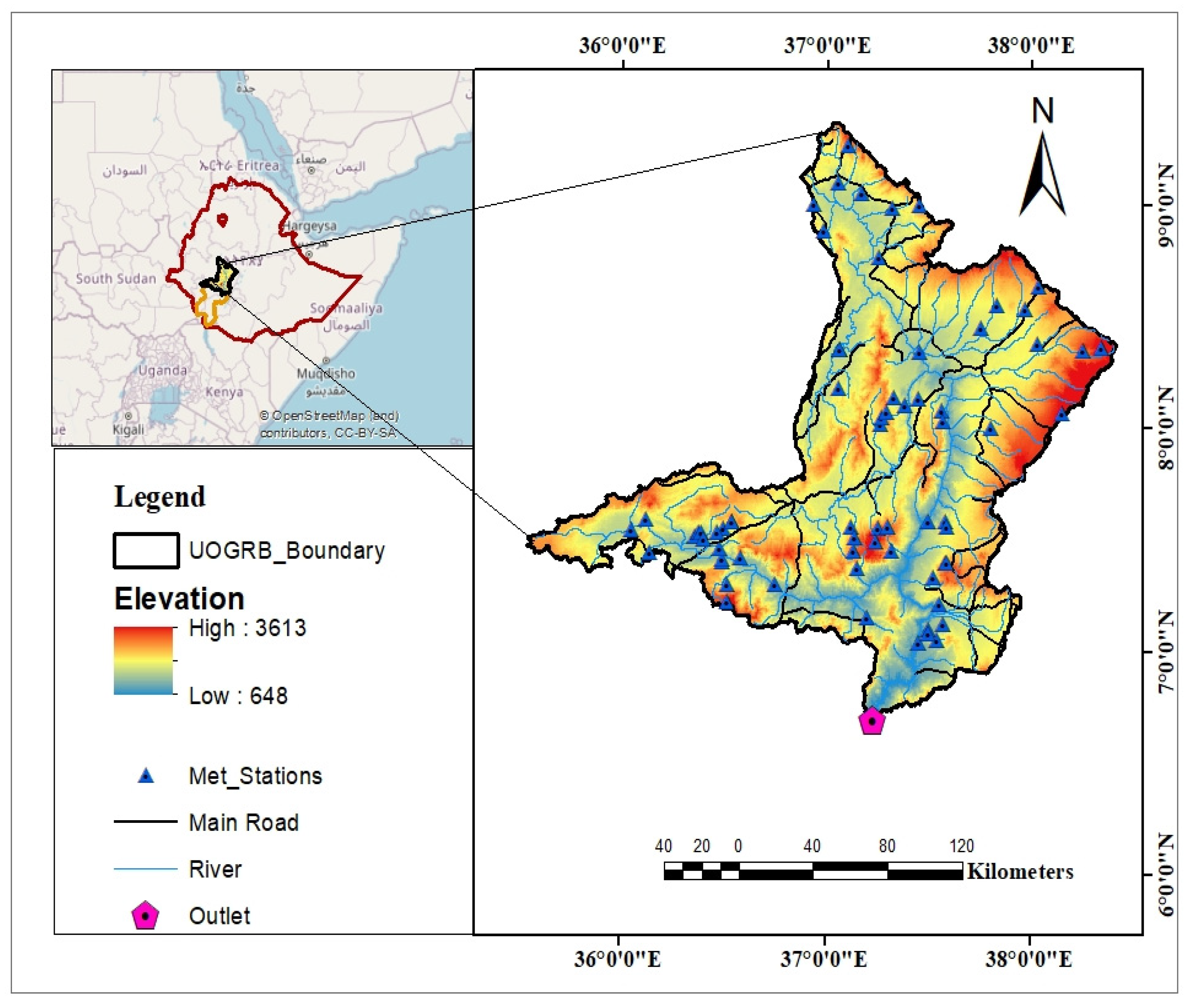
The Omo–Gibe River basin is one of the twelve river basins in Ethiopia. It covers 79,000 km² and is situated in three regional states: the Oromia regional state, Southern Nations, Nationalities and Peoples’ Region, and Southwest Ethiopia regional states. The basin is conventionally divided into two large subbasins: the Upper Omo–Gibe River basin and the Lower Omo–Gibe River basin. The Upper Omo–Gibe River basin (hereafter called UOGRB) covers a total area of 34,150 km² [40]. Geographically, it is located between 6°15′00″ and 9°50′00″ north latitude and 35°30′00″ and 38°45′00″ east longitude (Figure 1). It constitutes three hydroelectric power dams from Gilgel Gibe I to Gilgel Gibe III. Topographically, the basin is characterized by rugged terrain, mountains and valleys. The climate in the area is subhumid, and the main rainy season is between June and September, with a mean annual rainfall of 1300 to 2000 mm and an average temperature of 20.4 °C [41].

2.2. Materials

2.2.1. Data Acquisition and Preprocessing

The UOGRB watershed boundary (Figure 1) was extracted from the SRTM 30 m DEM, which was downloaded from http://earthexplorer.usgs.org/ (accessed on 17 October 2021). Temporal satellite imagery data were obtained from Landsat satellite series for the years 1991, 1997, 2004, 2010, 2016, and 2022. Landsat-5 TM for 1991 and 2004, Landsat-7 ETM+ for 2010, and Landsat-8 operational land imager (OLI) for 2016 and 2022 were downloaded from the USGS Earth Explorer Data Center (https://earthexplorer.usgs.gov/ (accessed on 4 February 2022)). For compatibility issues, the data were projected to the Universal Transverse Mercator (UTM) with data from the World Geodetic System 84 (WGS84), the projection system zone 37 N (

Table 1. Landsat satellite image acquisition and description.

S.N	Satellite	Sensor	Path	Row	Ground Resolution	Bands	Date of Acquisition
01	Landsat-5	TM *	169	054/055	30 m	7	10 January 1991
			170	054/055	30 m	7	18 February1991
02	Landsat-5	TM	169	054/055	30 m	7	14 January 2004
			170	054/055	30 m	7	15 February 2004
03	Landsat-7	ETM+ **	169	054/055	30 m	7	7 February 2010
			170	054/055	30 m	7	15 January 2010
04	Landsat-8	OLI ***	169	054/055	30 m	7	7 February 2016
			170	054/055	30 m	7	12 January 2016
04	Landsat-8	OLI	169	054/055	30 m	7	31 January 2022
			170	054/055	30 m	7	22 January 2022

* Thematic Mapper, ** Enhanced Thematic Mapper+, *** Operational Land Imager.

). The dry season (January to March) was chosen for the data selection to obtain the image data with the lowest cloud cover.

In this study, satellite images from different UTM zones (UTM Zone 36 N and UTM Zone 37 N) were used. To make image data compatible with each other, images were reprojected to the common geographic coordinate system using the world coordinate reference system (CRS: EPSG: 4326–WGS 84). Atmospheric, geometric, and radiometric corrections were performed in QGIS 3.22 and ERDAS IMAGINE 2014 software. To correct the scan line error (SLE) that occurred in the Landsat 7-ETM+ image due to the SLC-off [42] the Landsat toolbox was used.

2.2.2. Spatial Variable Identification and Preparation

Since they have a higher impact on the LULC change mechanisms, researchers pay particular attention to the physical and socioeconomic factors that contribute to LULC modifications [43]. It is obvious that geographical and climatic factors are thought to have the greatest influence on how people behave. The proximity to roads makes it easier to ascertain the motivations underlying the construction of the terrain. In this study, a variety of proximity and physical factors were considered.

The MOLUSCE plugin in QGIS offers several well-known techniques, including Pearson’s correlation and Cramer’s coefficient, for assessing the connection between LULC data and geographic factors [44]. Pearson’s correlation was used in the present study to measure the relationship between variables because the spatial variables employed were not categorical. Pearson’s correlation, r_p, is a parametric measure of the linear correlation between two variables, which was defined as the covariance of the two variables divided by the product of their standard deviations, as stated in [45]:

$${\mathrm{r}}_{\mathrm{p}} (\mathrm{X}, \mathrm{Y}) = \frac{\frac{{{\displaystyle \sum }}_{i=1}^n\left(xi- \overline{x}\right) \left(yi- \overline{y}\right)}{n-1}}{\sqrt{\frac{{{\displaystyle \sum }}_{i=1}^n{(xi- \overline{x})}^2}{n-1}\frac{{{\displaystyle \sum }}_{i=1}^n{(yi- \overline{y})}^2}{n-1}}} = \frac{{{\displaystyle \sum }}_{i=1}^n\left(xi-\overline{x}\right)\left(yi-\overline{y}\right)}{\sqrt{{{\displaystyle \sum }}_{i=1}^n{\left(xi-\overline{x}\right)}^2{{\displaystyle \sum }}_{i=1}^n{(yi-\overline{y})}^2}}$$

(1)

where the mean of each variable is subtracted from the raw scores in the numerator, and the cross-products of the centered variables are added up. The scales of the variables are changed by the denominator to have equal units. As a result, r is defined as the standardized and centered cross-product of two variables in Equation (1). Pearson’s correlation coefficient, r_p ranges from −1 to 1. A value of 0 implies no linear association between the two variables, whereas values of 1 and −1 imply perfect positive and negative associations between the two variables, respectively. Spatial variables chosen for this study with reference to previous studies [46] in association with the study area existing and potential features include altitude, slope gradient, population density, distance from the main road, distance from the rivers, and distance from the urban center.

2.3. Methods

2.3.1. Land Use/Land Cover Classification

After the data were preprocessed and the quality enhancement techniques were conducted, LULC classification (Figure 2) was performed using seven land use/land cover classes. LULC classes were categorized as forest (riparian vegetation, deciduous woodlands, dense forest, woodland, mixed forest, open forest, evergreen broad leaved forests, evergreen needle leaved forests, deciduous forest, and afro-alpines), agricultural land (cropland, farmland, plantation, and fallow land), water bodies (rivers, ponds, swamps, wetlands, and reservoirs), built-up areas (infrastructures include asphalt roads, houses, buildings, and urban areas), shrubland (open and closed shrublands), grassland (range land, open areas with vegetation less than 2 m in height, and savannas), and bare land (bare soil with no vegetation or plantation, silt, gravel, degraded hillsides, rock outcrops, and open lands without natural forests or crops) (

Table 2. LULC classes and description.

Land Use/Land Cover Type	Description
Forest	Evergreen broad-leafed and evergreen needle-leafed forest, deciduous, woodland, open forest, dense forest, and afro-alpine.
Agricultural land	Lands occupied by crops, farmland, plantation, and fallow land.
Waterbody	Rivers, ponds, swamps, and reservoirs.
Built-up area	Infrastructures include houses, asphalt roads, buildings, and urban areas.
Shrubland	Include open and closed shrublands.
Grassland	Open grass lands, vegetation less than 2 m height, and range lands.
Bare land	Lands without vegetation, crops or grasses, and barren soils.

).

2.3.2. Change Evaluation and Modeling Transition Potential

In this study, the MOLUSCE plugin in QGIS was utilized to simulate the LULC transition between LULC classes and estimate spatiotemporal changes for the five time periods (1991–1997, 1997–2004, 2004–2010, 2010–2016, and 2016–2022), and five LULC maps were produced. Area change and transition probability matrixes were generated using 2010 and 2016 LULC. The artificial neural network (ANN) multilayer perception strategy was employed. Elevation, slope gradient, population density, distance from the main roads, distance from the urban center, and distance from streams were considered in the study as the determinant factors for future land use/land cover change prediction. In LULC change analysis and prediction, these variables are frequently used because they provide verifiable information on the impact of anthropogenic and natural factors on LULC dynamics [48].

3. Results

3.1. LULC Classification

Based on the classes identified prior to the classification process, LULC for the years 1991, 1997, 2004, 2010, 2016, and 2022 was performed using the random forest classification algorithm [49] and (Figure 3). The LULC classification method has advanced over time by employing various machine learning algorithms, such as random forest (RF) [50] support vector machine (SVM) [51] maximum likelihood classifier (MLC) [17], and kNN [52]. Among the machine learning approaches, random forest is preferable for various reasons: better capability of handling outliers and data noises, better performance with multidimensional datasets from different sources, relatively better accuracy than other commonly used classifiers, such as kNN, SVM, and MLC [53], and optimized processing speed due to selection of effective variables [50]. In the random forest classification method [49] the number of trees (Ntree) and individual split-based features (Mtry) are needed. Many studies have stated that the random forest classifier is effective in LULC classification [37], resulting in accurate classification output. According to [19] a large number of trees can provide a sound result for variables. Various studies [54,55] have stated that better results can be obtained with the default number of trees (Ntree = 500) as in the QGIS random forest classifier, which works in combination with Sentinel Application Platform (SNAP) software integrated into the classification algorithm.

3.2. Classification Accuracy Assessment

After the images were classified using the random forest classification algorithm, the next step employed was image classification accuracy assessment [56]. Accuracy assessment is considered a component of the image classification method that enables the researcher to check whether the classification result has a strong, medium, or poor agreement with the ground truth [57]. It helps assess the classification methodology and is crucial for identifying any potential errors. In the form of a confusion matrix, the classifier’s accuracy was evaluated (

Table 3. Confusion matrixes for LULC classification (i) 1991, (ii) 1997, (iii) 2004, (iv) 2010, (v) 2016, and (vi) 2022.

(i)			Reference Data
		LULC Cat.	Forest	AgrL	WB	BuA	ShL	GrL	BrnL	RTotal	UA
LULC 1991	Classified Data	Forest	69	0	0	0	2	1	0	72	0.97
		AgrL	5	64	0	0	1	1	0	71	0.90
		WB	29	8	34	0	1	0	0	72	0.47
		BuA	5	0	0	65	0	1	1	72	0.92
		ShL	7	1	2	0	63	0	1	74	0.85
		GrL	1	2	0	1	0	68	0	72	0.94
		BrnL	4	4	0	0	4	2	57	71	0.80
		CTotal	120	79	36	66	71	73	59	504
		PA	0.58	0.82	0.94	0.98	0.9	0.93	0.97
(ii)			Reference Data
		LULC Cat.	Forest	AgrL	WB	BuA	ShL	GrL	BrnL	Total	UA
LULC of 1997	Classified Data	Forest	57	14	0	0	2	0	0	73	0.79
		AgrL	0	69	1	0	1	1	0	72	0.96
		WB	22	3	46	0	0	0	0	71	0.65
		BuA	0	2	1	69	0	0	0	72	0.96
		ShL	0	6	0	0	66	0	0	72	0.92
		GrassL	0	7	0	0	0	65	0	72	0.90
		BarrenL	0	8	0	0	0	0	64	72	0.89
		Total	79	109	48	69	69	66	64	504
		PA	0.72	0.63	0.96	1	0.97	0.98	1	0	0.87
(iii)			Reference Data
		LULC Cat.	Forest	AgrL	WB	BuA	ShL	GrL	BrnL	Total	UA
LULC of 2004	Classified Data	Forest	72	0	0	0	0	0	0	72	1
		AgrL	3	67	0	0	1	0	0	71	0.94
		WB	6	13	53	0	0	0	0	72	0.74
		BuA	0	2	0	70	0	0	0	72	0.97
		ShL	0	0	0	1	71	1	0	73	0.99
		GrL	0	0	0	0	0	72	0	72	1
		BrnL	3	0	0	0	0	0	69	72	0.96
		Total	84	82	53	71	72	73	69	504	0
		PA	0.86	0.82	1	1	1	0.99	1	0	0.94
(iv)			Reference Data
		LULC Cat.	Forest	AgrL	WB	BuA	ShL	GrL	BrnL	Total	UA
LULC 2010	Classified Data	Forest	66	4	1	0	2	0	0	73	0.90
		AgrL	3	67	0	0	1	0	0	71	0.94
		WB	17	0	54	0	1	0	0	72	0.76
		BuA	1	2	1	68	1	0	0	73	0.93
		ShL	1	1	0	1	71	0	0	74	0.96
		GrL	0	0	0	0	0	71	0	71	1
		BrnL	0	0	0	0	0	0	70	70	1
		Total	88	74	56	69	76	71	70	504
		PA	0.77	0.91	0.96	1	0.93	1	1
(v)			Reference Data
		LULC Cat.	Forest	AgrL	WB	BuA	ShL	GrL	BrnL	Total	UA
LULC 2016	Classified Data	Forest	66	6	0	0	0	0	0	72	0.92
		AgrL	0	69	0	1	1	1	0	72	0.96
		WB	3	3	66	0	0	0	0	72	0.92
		BuA	0	0	0	72	0	0	0	72	1
		ShL	0	4	0	0	68	0	0	72	0.94
		GrL	0	5	0	1	0	66	0	72	0.92
		BrnL	12	0	0	0	0	0	60	72	0.83
		Total	81	87	66	74	69	67	60	504	0
		PA	0.81	0.79	1	0.97	0.99	0.99	1	0	0.93
(vi)			Reference Data
			Forest	AgrL	WB	BuA	ShL	GrL	BrnL	Total	UA
LULC 2022	Classified Data	FRST	71	0	0	0	0	0	0	71	1
		AGRL	2	68	0	0	1	1	0	72	0.94
		WB	2	0	74	0	1	0	0	77	0.97
		BUA	0	10	0	58	2	1	0	71	0.82
		SHL	2	0	0	0	70	0	0	72	0.97
		GL	0	2	0	0	0	69	0	71	0.97
		BL	0	0	0	0	0	0	70	70	1
		Total	77	80	74	58	74	71	70	504
		PA	0.93	0.85	1	1	0.96	0.97	1

AgrL = agricultural land, WB = waterbody, BuA = built-up area, ShL = shrubland, GrL = grassland, BrnL = barn land, PA= producer’s accuracy, UA = user’s accuracy.

). The accuracy evaluation of each classification generated by the random forest-based classification was performed in the present study utilizing random points extracted using the classification and segmentation toolsets in the Spatial Analyst tools of ArcGIS and verified using historical Google Earth images.

The accuracy for LULC classification was assessed using the statistical tool known as the Kappa coefficient, as shown in

Table 4. Classification degree of agreement.

Year	Over All Accuracy (%)	Kappa Coefficient	Degree of Agreement (%)
1991	82	0.81698	Almost perfect agreement
1997	87	0.85296	Almost perfect agreement
2004	94	0.94348	Almost perfect agreement
2010	93	0.93179	Almost perfect agreement
2016	93	0.914352	Almost perfect agreement
2022	95	0.94825	Almost perfect agreement

. According to [58], a classification has low agreement if the kappa coefficient value is less than 0.4, medium agreement if it is between 0.4 and 0.8, and good agreement if it is over 0.8. For the LULC classification in 1991, the kappa coefficient was 0.83 (83%) in 1997, 0.87 (87%) in 2004, and 0.94 (94%); in 2010, it was 0.93 (93%) in 2016 and 0.93 (93%); and in 2022, it was 0.95 (95%). According to the classification results, the 2022 LULC classification had the highest degree of agreement (95%), while the 1991 LULC classification had the lowest degree of agreement. The quality of the data was what caused the disparity. Comparatively, the 1991 Landsat-5 TM (Thematic Mapper) image has lower quality than the 2022 Landsat-8 (OLI) image, which influences the quality of LULC classification.

3.3. LULC Change Analysis and Evaluation

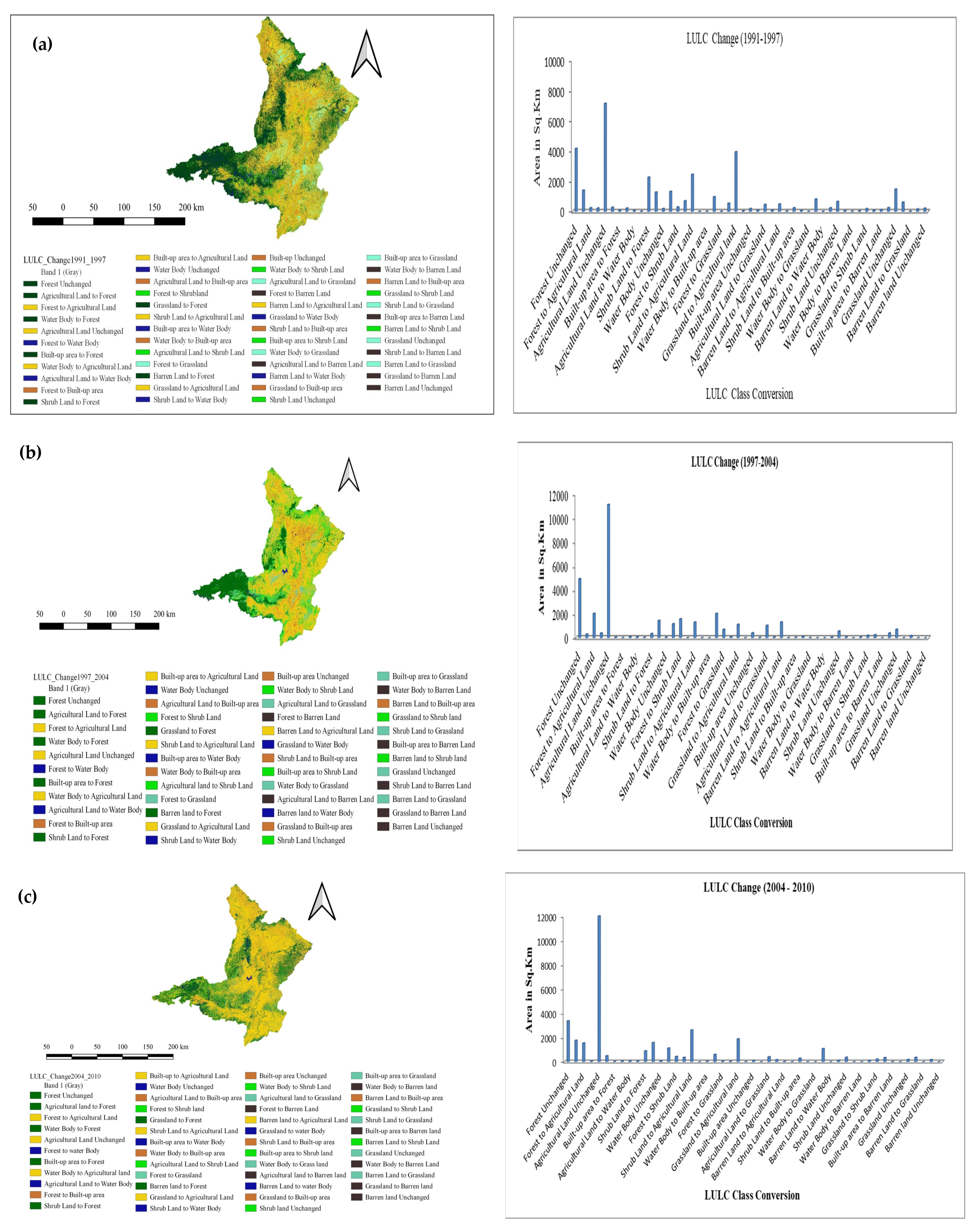
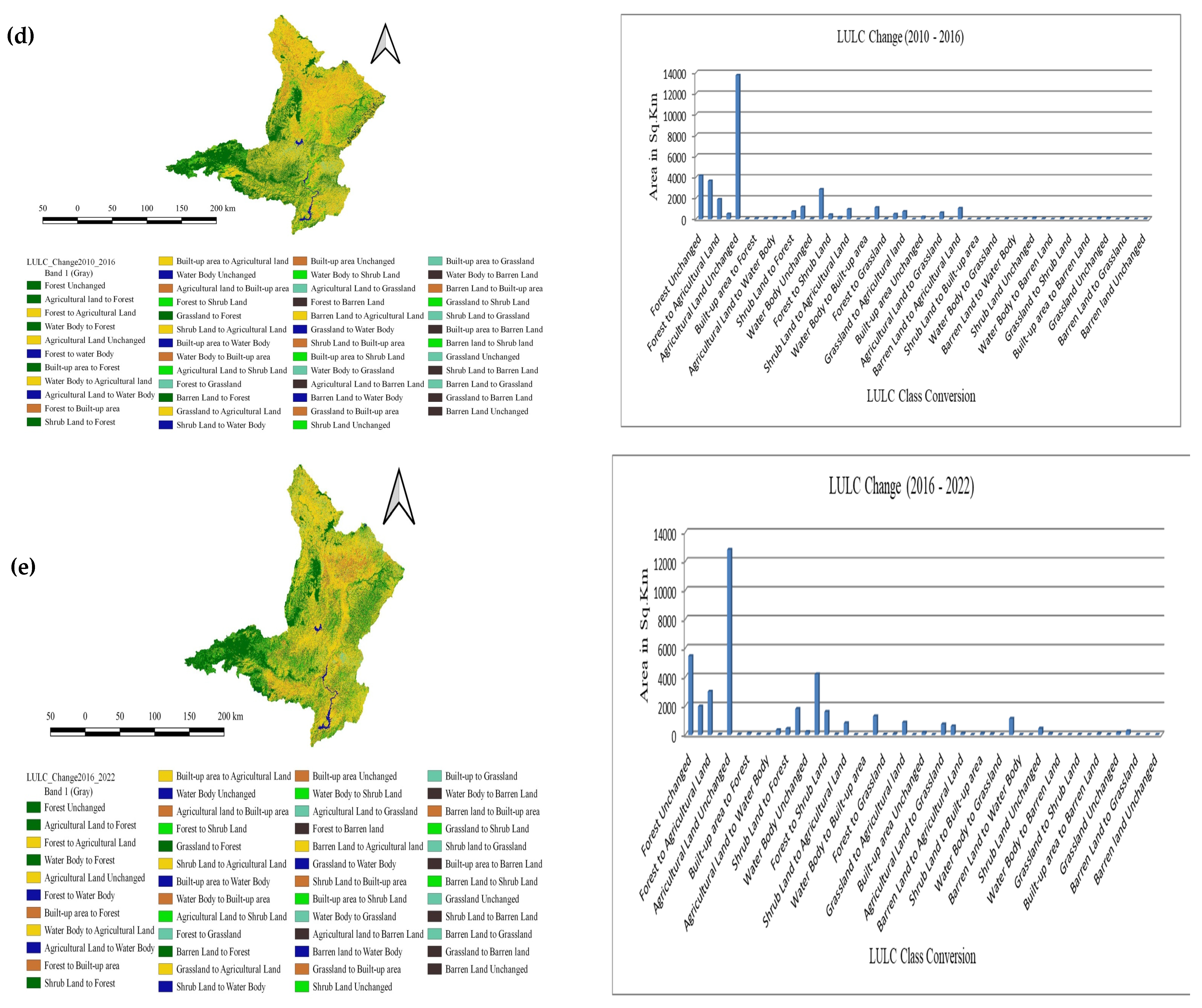
After the accuracy assessment was conducted and the classification status was evaluated based on the kappa value for each year, change detection for 1991–1997, 1997–2004, 2004–2010, 2010–2016, and 2016–2022 was performed using QGIS 3.22 software. Change detection, as shown in Figure 4, was presented using maps and bar graphs. From 1991 to 1997, forest and agricultural land showed a high increase in area, and built-up area and shrubland showed less change in area coverage (

Table 5. LULC area (km²) from 1991 to 2022.

	1991		1997		2004		2010		2016		2022
LULC Cat.	Area (km2)	Area (%)	Area (km2)	Area (%)	Area (km2)	Area (%)	Area (km2)	Area (%)	Area (km2)	Area (%)	Area (km2)	Area (%)
Forest	5026	15	9372	27	6028	18	6483	19	9768	28	5004	15
AgrL	12,032	36	15,736	46	18,275	53	21,219	62	19,536	57	22,147	65
WB	729	2	567	2	257	1	652	2	281	1	277	1
BuA	1776	5	2037	6	1812	5	1529	4	2025	6	2559	7
ShL	6255	18	2476	7	4841	14	1632	5	1791	5	2398	7
GrL	6629	19	2091	6	2903	8	981	3	772	2	859	3
BrnL	1515.87	4	2007	6	172	1	1791	5	113	0	1044	3

and

Table 6. LULC change analysis in 7-year intervals from 1991 to 2022.

	1991–1997		1997–2004		2004–2010		2010–2016		2016–2022
LULC Cat.	Area (km2)	Change (%)	Area (km2)	Change (%)	Area (km2)	Change (%)	Area (km2)	Change (%)	Area (km2)	Change (%)
Forest	12,717	37	−3344	−10	456	1	3285	10	−4764	−14
AgL	13,197	38	2539	7	2945	9	−1684	−5	2611	8
WB	878	3	−311	−1	395	1	129	0	112	0
BuA	263	1	1775	5	−284	−1	497	1	1544	5
ShL	111	0	2365	7	−3209	−9	159	0	607	2
GrL	1279	4	812	2	−1922	−6	−209	−1	87	0
BrnL	3841	11	−1835	−5	1619	5	−1678	−5	931	3

). Between 2016 and 2022, the forestland showed a dramatic change (decreased) in area, and the built-up area greatly increased (Table 6).

3.4. Spatial Variables

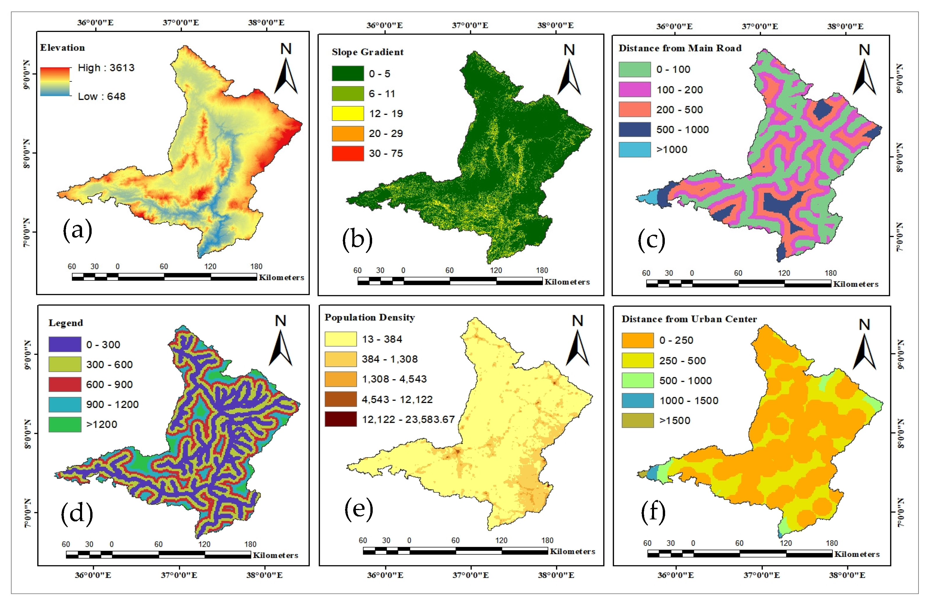
The spatial variables selected for the current study are altitude, slope gradient, distance from the main roads, distance from the streams, population density, and the distance from the urban centers based on previous studies [59]. After relevant spatial variables (Figure 5) were selected and factor maps were created, geometry matching was conducted, which included the cell size of the raster data, NoData value, data extent, dimension, and coordinate reference system. The cell size, NoData value, and coordinate reference system are 30 m, 0, and WGS_1984_UTM_Zone_37 N, respectively, for all spatial variables.

In this study, Pearson’s correlation was used to measure the correlation between variables. The MOLUSCE plugin in QGIS provided three options for correlation measurement: Pearson’s correlation, Cramer’s coefficient, and joint information uncertainty [60]. Pearson correlation was chosen because the variables used in this study are not categorical.

Table 7. Evaluation of the correlation between variables using Pearson’s correlation method.

Spatial Variables	Elev	Dmrd	SlpGt	DStr	Pdsty	DUC
Elevation (Elev)		0.038	0.005	0.525 *	0.037	0.109
DistMainRoad (Dmrd)			0.153	−0.025	0.045	0.609 *
Slope Gradient (SlpGt)				0.084	0.026	0.059
DistStreams (DStr)					0.031	0.016
Population Density (Pdsty)						0.072
DistUrbanCenter (DUC)

DistMainRoad = distance from the main road, DistStreams = distance from the streams, DistUrbanCenter = distance from the urban center. * Are strongly correlated variables.

indicates that elevation, distance from the main road, and distance from the urban center are more strongly correlated than other variables, so these variables were selected for LULC change simulation and prediction.

3.5. LULC Change Simulation and Prediction Using the CA-ANN Model

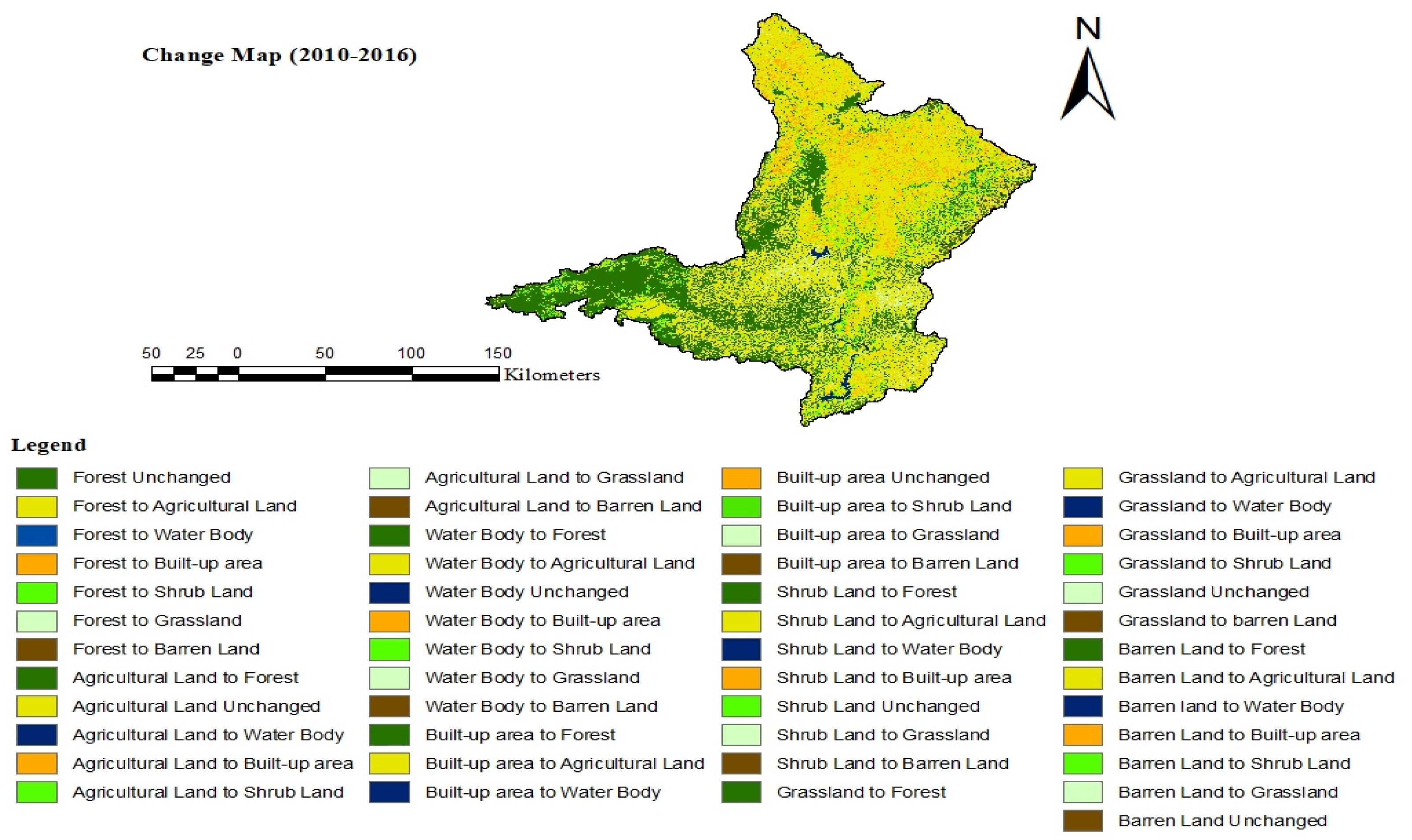
The QGIS MOLUSCE plugin provided artificial neural network (ANN) and cellular automata (CA) machine learning algorithms for LULC change simulation and prediction. ANN follows the nonparametric, nonlinear, and stochastic approach in LULC change simulation and prediction, which processes the potential to solve problems emanating from different variables [61]. Using its capacity to learn from a large number of datasets, ANN enabled the model to manage complex conditions during simulation. ANN basically uses the multilayer perception (MLP) approach [62] considering previously recorded LULC changes and spatial variables (explanatory variables) for LULC modification. In this study, the LULC of 1991, 1997, 2004, 2010, 2016, and 2022 (

Table 8. Transition matrix of 1991–2022.

1991		1997
		Forest	AgrL	WB	BuA	ShL	GL	BL
	Forest	0.586	0.063	0.007	0.029	0.351	0.096	0.008
	AgrL	0.014	0.603	0.023	0.016	0.141	0.199	0.004
	WB	0.364	0.124	0.240	0.002	0.181	0.080	0.009
	BuA	0.005	0.641	0.001	0.027	0.061	0.252	0.012
	ShL	0.056	0.342	0.004	0.011	0.241	0.33	0.013
	GL	0.012	0.492	0.001	0.149	0.039	0.259	0.043
	BL	0.043	0.316	0.003	0.007	0.253	0.390	0.009
1997		2004
		Forest	AgrL	WB	BuA	ShL	GL	BL
	Forest	0.472	0.352	0.221	0.003	0.034	0.004	0.023
	AgrL	0.049	0.809	0.003	0.070	0.019	0.018	0.030
	WB	0.435	0.462	0.052	0.018	0.015	0.003	0.014
	BuA	0.007	0.854	0.003	0.081	0.004	0.042	0.009
	ShL	0.373	0.389	0.016	0.010	0.113	0.022	0.076
	GL	0.123	0.591	0.004	0.036	0.073	0.058	0.107
	BL	0.078	0.714	0.007	0.045	0.056	0.241	0.073
2004		2010
		Forest	AgrL	WB	BuA	ShL	GL	BL
	Forest	0.631	0.412	0.016	0.014	0.234	0.007	0.061
	AgrL	0.137	0.619	0.008	0.061	0.078	0.037	0.059
	WB	0.736	0.081	0.088	0.004	0.069	0.001	0.020
	BuA	0.070	0.760	0.001	0.060	0.038	0.044	0.037
	ShL	0.310	0.359	0.001	0.018	0.210	0.006	0.094
	GL	0.115	0.703	0.001	0.010	0.070	0.065	0.035
	BL	0.321	0.634	0.004	0.021	0.210	0.083	0.077
2010		2016
		Forest	AgrL	WB	BuA	ShL	GL	BL
	Forest	0.633	0.271	0.007	0.011	0.067	0.007	0.003
	AgrL	0.174	0.647	0.008	0.087	0.052	0.029	0.002
	WB	0.757	0.115	0.083	0.004	0.034	0.003	0.005
	BuA	0.051	0.756	0.002	0.132	0.036	0.023	0.000
	ShL	0.448	0.445	0.002	0.012	0.074	0.014	0.004
	GL	0.199	0.640	0.003	0.024	0.026	0.098	0.010
	BL	0.277	0.578	0.006	0.031	0.076	0.019	0.013
2016		2022
		Forest	AgrL	WB	BuA	ShL	GL	BL
	Forest	0.870	0.130	0	0	0	0	0
	AgrL	0.142	0.858	0	0	0	0	0
	WB	0.952	0.044	0.004	0	0	0	0
	BuA	0.006	0.987	0	0.007	0	0	0
	ShL	0.188	0.698	0	0	0.114	0	0
	GL	0.069	0.916	0	0	0	0.015	0
	BL	0.290	0.676	0	0	0	0	0.034
2022		2037
		Forest	AgrL	WB	BuA	ShL	GL	BL
	Forest	0.999	0.001	0	0	0	0	0
	AgrL	0.001	0.999	0	0	0	0	0
	WB	0.002	0	0.998	0	0	0	0
	BuA	0.000	0.000	0	1.000	0	0	0
	ShL	0.026	0.004	0	0	0.970	0	0
	GL	0.001	0.002	0	0	0	0.998	0
	BL	0	0	0	0	0	0	1

AgrL = agricultural land, WB = waterbody, BuA = built-up Area, ShL = shrubland, GL = grassland, BL = bare land.

) and six spatial variables, including altitude, slope gradient, distance from the main road, distance from the streams, population density, and distance from the urban center, were considered as inputs for model simulation using the MOLUSCE plugin in QGIS. The initial and final rasters were the LULC maps of 2010 and 2016, respectively, to simulate 2022 LULC. The simulation model was constructed, and verification was performed for 2022. A change map was created using 2010 and 2016 LULC maps (Figure 6).

As indicated in Figure 7, agricultural land expanded, and forest cover, shrubland, and bare land decreased from 1991 to 1997. From 1997 to 2004, forest cover and agricultural land increased, but shrubland and grassland decreased. From 2016 to 2022, agricultural land and built-up areas showed a dramatic expansion, but forest cover, water bodies, shrubland, and bare land decreased in size (Figure 7).

3.6. Artificial Neural Network (ANN)-Based LULC Change Transition Potential Modeling

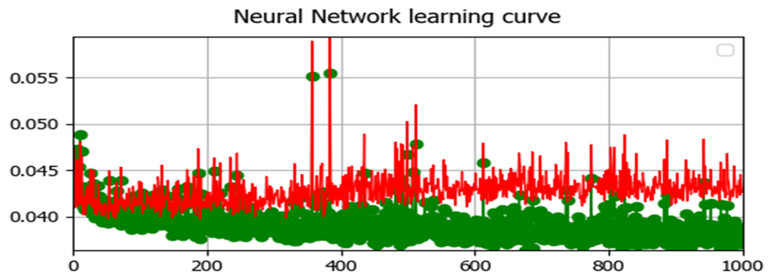
Based on MOLUSCE’s approach, transition potential modeling was conducted using an artificial neural network (ANN), which is ruled by the multilayer perception method employing neighborhood (1 px), learning rate (0.01) (Figure 8), maximum iteration (1000), hidden layer (12), momentum (0.05), fixed overall accuracy (−0.0018), minimum error for validation (0.0317), and validation kappa (0.9781). The model used 5000 randomly distributed samples to provide spatial representation for ANN. Based on the fixed value (0.01 learning rate), the neural network learned and simulated LULC changes for 2022.

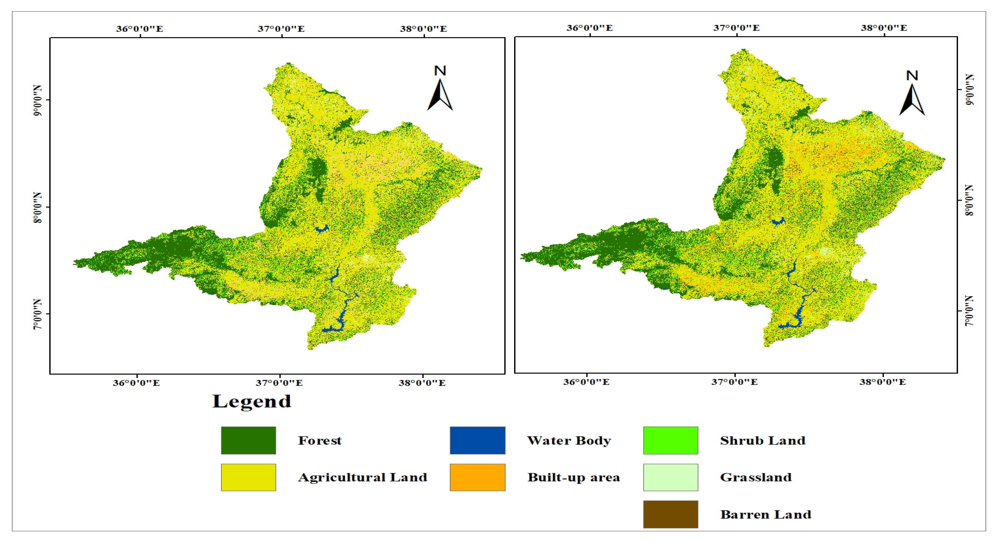
Transition potential modeling was computed, and future LULC changes were predicted using the CA-ANN model. The model utilized LULC data from 2010 to 2016 to predict the change in 2022, which resulted in a validation kappa value of 0.97. An overall accuracy of 87% and an overall kappa value of 0.82 were obtained by comparing the actual data of 2022 with the simulated LULC data from the same year. The actual and simulated LULC maps for 2022 are indicated in Figure 9 and their areal coverage was presented in

Table 9. Actual and simulated LULC of 2022.

LULC Category	Actual		Simulated
	Area (km2)	Area (%)	Area (km2)	Area (%)
Forest	5004	13	4371	10
Agricultural land	22,147	58	28,314	63
Waterbody	893	2	938	2
Built-up area	5569	15	7658	17
Shrubland	2398	6	2149	5
Grassland	859	2	678	2
Barren land	1044	3	984	2

.

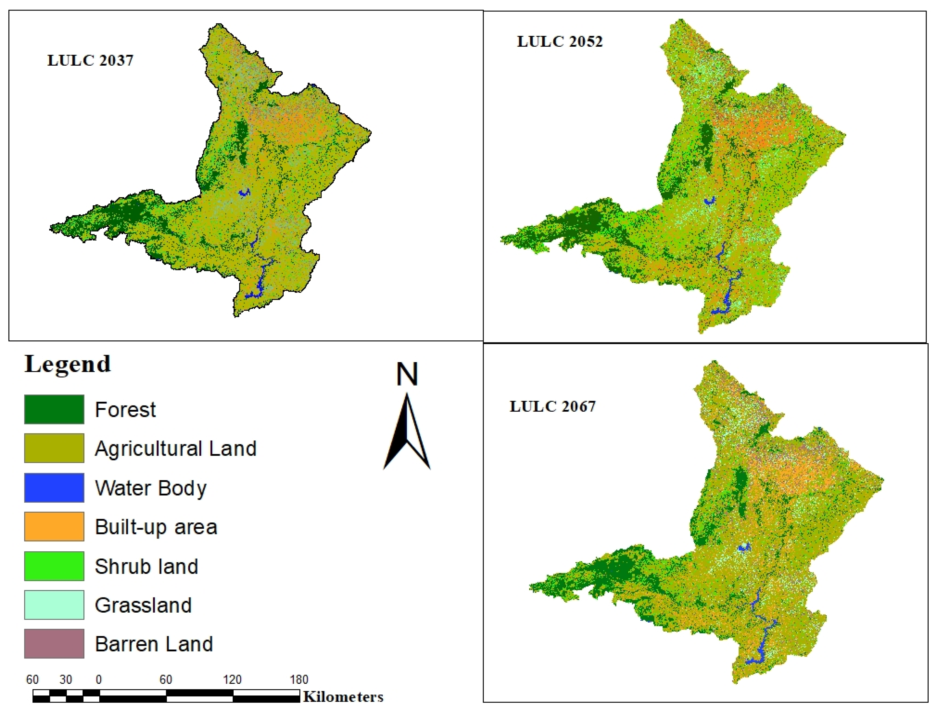
3.7. LULC Prediction

The LULC predictions for 2037, 2052, and 2067 (Figure 10 and

Table 10. Area in km² for the LULC (2037, 2052, and 2067).

	LULC2037		LULC2052		LULC 2067
LULC Cat.	Area (km2)	Area (%)	Area (km2)	Area (%)	Area (km2)	Area (%)
Forest	5139	15	4872	14	4328	13
Agricultural land	22,146	64	21,273	62	22,353	65
Waterbody	273	1	272	1	293	1
Built-up area	1725	5	2749	8	2858	8
Shrubland	1859	5	1763	5	1572	5
Grassland	1787	5	1674	5	1561	5
Barren land	1895	5	1684	5	1473	4

) were performed after obtaining acceptable model validation results. The procedure of model validation combines the contents of two data sources and takes into consideration the features of actual and simulated LULC data. The LULC for 2037 was predicted using the LULC data between 2016 and 2022, the spatial variables selected for simulation, and the transition probability matrix, and a kappa value of 0.73 was attained. Consequently, LULC for 2052 was predicted using the LULCs of 2022 and 2037, employing the explanatory factors and transition matrix, and the kappa value computed was 0.68. Finally, using the projected data for 2052–2067 and the transition matrix, we forecasted the LULC for 2082 and arrived at a kappa value of 0.69 as a result.

3.8. Change Prediction

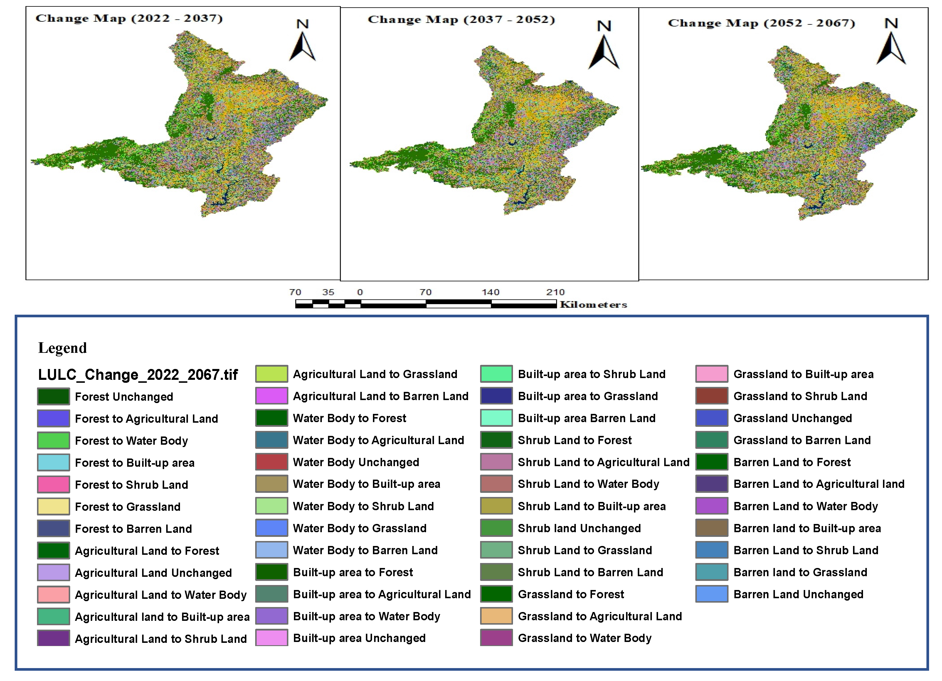
The evaluation performed on LULC changes during the course of the investigation showed significant changes across land LULC classes. The results from 2022 to 2067 demonstrate a discernible increase in built-up areas and a decrease in forest cover and shrubland. The area coverage and percentage changes for each LULC category are presented in Figure 11 and

Table 11. LULC changes from 2037 to 2067.

	2022–2037		2037–2052		2052–2067
LULC Cat	km2	%	km2	%	km2	%
Forest	−16,492	−48	−267	−1	−544	−2
Agricultural land	21,631	63	−873	−3	1079	3
Waterbody	515	2	−1	0	21	0
Built-up area	115	0	1024	3	109	0
Shrubland	1967	6	−96	−0	−191	−1
Grassland	−107	−0	−113	−0	−113	−0
Barren land	1895	6	−211	−1	−210	−1

. Inter-transitions between LULC classes and their contribution to other classes intensify changes in LULC at times. As indicated in Table 11, between 2022 and 2037, agricultural land (2163 km², 63%) and shrubland (1966 km², 5%) showed a significant increase, and forest (−1649, −48%) and grassland (−107 km², −0.31%) decreased. From 2037 to 2052, the built-up area of 1023 km² (3%) showed a significant increase, and forest −267 km² and agricultural land of −873 km² (−3%) showed a significant decrease. From 2052 to 2067, the projected LULC simulation result showed that agricultural land (1079 km², 3%) and built-up area (109 km², 0.32%) increased and forest −544 km² (−2%) and shrubland −191 km² (−1%) showed significant decreases.

4. Discussion

Recently, most of the changes occurring in the physical and human environments have been directly related to the changes emanating from LULC dynamics. This condition has attracted the interest of scholars from academic and research institutes globally. In this regard, an ample number of studies have been conducted [63,64] dealing with the impact of LULC changes on various aspects of the environment. Water resource (surface and subsurface) availability, climate variability, soil fertility, and agricultural productivity are some of the phenomena directly or indirectly influenced by LULC changes. Climate variability may have a negative impact on land use and cover, as well as alter the environment’s natural aesthetic. Lack of rainfall and temperatures that are abnormally high or low have detrimental impacts on the ecosystem [34].

The expansion of anthropogenic activities due to newly commenced national and international projects contributes greatly to environmental alteration, paving the way for the intensification of LULC changes. The study conducted in Linyi, China, considering land use/land cover change analysis, evaluation, and prediction using the QGIS MOLUSCE plugin and remote sensing big data revealed an increase in the population number and density; and the associated expansion of urban areas significantly caused a decrease in forest resource and grasslands [65].

In the Ethiopian context, population growth is the leading factor for LULC changes, which contributes to land fragmentation, forest loss, and loss of biodiversity. LULC dynamics can be primarily attributed to a variety of anthropogenic activities, including the encroachment of farmland into vegetated lands, the growth of farm plots at the expense of forestlands, the massive production of fuelwood and charcoal to support livelihood, overgrazing, and the expansion of farm plots into agricultural lands.

The study undertaken in Nashe Watershed, Upper Blue Nile Basin, Ethiopia, considered the prediction of land use/land cover changes using a land change modeler. This study used Landsat imageries for land use/land cover classification and predicted future LULC changes using the CA-Markov model. The study findings revealed that there will be a rapid conversion of forest land, range land, and grassland to agricultural land and built-up areas in the future and require a national policy implementation in order to maintain the goal of sustainable development [66]

The present study area, the Upper Omo–Gibe River basin, is known for its long mountain ranges, deep gorges, physically interconnected subbasins, lowland plains, woodlands, broad- and needle-leafed trees and grasslands, an enormous number of wild species, and mineral-rich soil [10]. Due to the existence of these environmental features in the study area, it was imperative to include spatial variables, such as elevation, slope gradient, distance from the river, and distance from the main road in the LULC change simulation and prediction.

According to the Gibe III hydroelectric project [67], the land cover of the study area comprises forest (open and dense forest, woodland, riverine forest, and plantation), agricultural land (cultivation, recession agriculture, fallow land, and croplands), water bodies, built-up areas, shrubland, grassland, and bare soil.

The present study considered seven land use/land cover classes, including forest, agricultural land, water bodies, built-up areas, shrubland, grassland, and barren land in reference to Landsat image time series data and some supportive sources, such as published and unpublished documents, topographic maps, and historical and current Google Earth images. Geospatial data for LULC classification were acquired from different sources. Digital elevation data with 30 m ground resolution were acquired from the shuttle radar topographic mission (SRTM). Landsat-5 TM for 1991 and 2004, Landsat-7 ETM+ for 2010, and Landsat-8 operational land imager (OLI) for 2016 and 2022 were downloaded from the USGS Earth Explorer Data Center. Spatial variables selected for the study were altitude, slope gradient, distance from the main roads, population density, distance from the streams, and distance from the urban center. Among the machine learning approaches, random forest is preferable for various reasons: better capability of handling outliers and data noises, better performance with multidimensional datasets from different sources, relatively better accuracy than other commonly used classifiers, such as kNN, SVM, and MLC, and optimized processing speed due to selection of effective variables.

The LULC classification result was evaluated using an accuracy assessment technique to assure the correctness of the classification method employing the kappa coefficient. Based on the classification evaluation outcome of the study, the kappa value for 1991 is 0.82 (82%), 1997 is 0.85 (85%), 2004 is 0.94 (94%), 2010 is 0.93 (93%), 2016 is 0.91 (91%), and 2022 is 0.95 (95%). Kappa coefficient values of the classification indicate that there was strong agreement between the classified and reference data.

The present study used the CA-ANN model for the evaluation and prediction of LULC changes in the future and found that the model is effective and reliable. However, it is suggested that further studies could employ more spatial and socioeconomic variables such as climate variability, economic development, technological advancement, political economy, and GDP (gross domestic product) to provide more sufficient and valuable information regarding the positive and negative impacts of LULC changes in the future.

5. Conclusions

LULC change detection was carried out for the time periods 1991–1997, 1997–2004, 2004–2010, 2010–2016, and 2016–2022, and the results were presented in maps and graphs. Landsat time series imageries were used to develop information classes based on the LULC categories. Raster data geometries were checked prior to simulation. The data extent, coordinate system, and NoData value were made to have the same content for simulation. Pearson’s correlation was used to measure the correlation between variables. Future LULC changes were predicted employing spatial and socioeconomic variables, such as elevation, slope gradient, distance from the main road, distance from streams, and population density, respectively, using the MOLUSCE plugin of QGIS and the CA-ANN model. The following conclusions were made based on the study’s findings.

Artificial neural network (ANN) and cellular automata (CA) machine learning methods were made available for LULC change modeling and prediction via the QGIS MOLUSCE plugin. ANNs have the potential to handle issues arising from many variables using nonparametric, nonlinear, and stochastic methods for LULC change modeling and prediction. The model was able to control complicated situations during simulation because ANN has the ability to learn from a large number of datasets. ANN primarily employs the multilayer perception (MLP) method while taking into account previously observed LULC changes and spatial variables (explanatory variables) for LULC modification. Transition potential modeling was computed, and future LULC changes were predicted using the CA-ANN model. The model utilized LULC data from 2010 to 2016 to predict the change in 2022, which resulted in a validation kappa value of 0.97. An overall accuracy of 86.53% and an overall kappa value of 0.82 were obtained by comparing the actual data of 2022 with the simulated LULC data from the same year and this result proved the reliability of the model.

The present study findings revealed that between 2022 and 2037, agricultural land increased by 2163 km² (or 63%) and shrubland by 1967 km² (or 6%) whereas grassland decreased by 107 km² (or 0.31%) and forest by 1650 km² (or 48%). From 2037 to 2052, the built-up area (1024 km²) (3%) showed a considerable increase, while the forest (−267 km²) and agricultural land (−873 km²) (3%) showed a significant decline. The predicted LULC simulation result from 2052 to 2067 revealed that while built-up area 109.05 km² (0.32%) and agricultural land 1079.28 km² (3.15%) both increased, forest −544.11 km² (−2%) and shrubland −191 km² (−1%) significantly decreased.

The results of the study show that the future physical and human environment will be impacted by the quick and intense LULC transformation. Due to this condition, the study catchment (Gibe-III catchment) will experience climate variability, soil erosion, biodiversity loss, scarcity of water resources (both surface and subsurface), drought susceptibility, disruption of water balance components, and reservoir sedimentation in the future. In addition, increased human population density in the study area, particularly in urban areas and areas near main roads, has led to extraordinary levels of land pressure and increased demand for vast amounts of land for the building of residential homes both in urban and rural areas.

Therefore, it is crucial to call for the development of long-run local and national plans and their implementation regarding the utilization of natural resources and land use in order to safeguard the natural resources and maintain the water balance of the study area in particular and the entire basin (Omo–Gibe River basin) in general. Studies such as this one will significantly contribute to bringing about the best resource usage in the future by offering timely and relevant information in regard to LULC change evaluation and monitoring; and its impact on the physical and human environment.

Finally, the predicted conditions in this study particularly the negative impacts of LULC changes may be overturned through the implementation of integrated local and regional scale policies and strategies toward efficient resource utilization, land use, and physical and human environmental protection. In line with this, practicing effective soil and water conservation measures, climate-resilient agricultural activities, periodic afforestation, and reforestation programs will tackle the adverse impacts emanating from the LULC changes. It is recommended that future studies undertake multisource data, more variables (spatial and socioeconomic), and models to evaluate and predict LULC changes, and provide sound information in the entire basin (Omo–Gibe River basin) and other basins.

References

1. Ayele, G.T.; Demessie, S.S.; Mengistu, K.T.; Tilahun, S.A.; Melesse, A.M. Multitemporal Land Uscape /Dynamics, Soils and Hydrological Processes in Varierd Change Detectlion for the Bmatena Watershed, Rift Valley Lakes Basin, Ethiopia Author Multitemporal Land Use / Land Cover Change Detection for the Batena Watershed, Rift Valley Lakes Basin, Ethiopia; Springer International Publishing: Cham, Switzerland, 2016. [Google Scholar] [CrossRef]
2. Welde, K.; Gebremariam, B. Effect of land use land cover dynamics on hydrological response of watershed: Case study of Tekeze Dam watershed, northern Ethiopia. Int. Soil Water Conserv. Res. 2017, 5, 1–16. [Google Scholar] [CrossRef]
3. Halmy, M.W.A.; Gessler, P.E.; Hicke, J.A.; Salem, B.B. Land use/land cover change detection and prediction in the north-western coastal desert of Egypt using Markov-CA. Appl. Geogr. 2015, 63, 101–112. [Google Scholar] [CrossRef]
4. Hyandye, C.; Martz, L.W. A Markovian and cellular automata land-use change predictive model of the Usangu Catchment. Int. J. Remote Sens. 2017, 38, 64–81. [Google Scholar] [CrossRef]
5. Khan, Z.; Saeed, A.; Bazai, M.H. Land use / land cover change detection and prediction using the CA-Markov model: A case study of Quetta city, Pakistan. J. Geogr. Soc. Sci. 2020, 2, 164–182. [Google Scholar]
6. Da Cunha, E.R.; Santos, C.A.G.; da Silva, R.M.; Bacani, V.M.; Pott, A. Future scenarios based on a CA-Markov land use and land cover simulation model for a tropical humid basin in the Cerrado/Atlantic forest ecotone of Brazil. Land Use Policy 2021, 101, 105141. [Google Scholar] [CrossRef]
7. Yifru, B.A.; Chung, I.-M.; Kim, M.-G.; Chang, S.W. Assessing the Effect of Land/Use Land Cover and Climate Change on Water Yield and Groundwater Recharge in East African Rift Valley using Integrated Model. J. Hydrol. Reg. Stud. 2021, 37, 100926. [Google Scholar] [CrossRef]
8. Cherie, W.D. Assessing the Impacts of Land use / cover Change on the Hydrological Response of Temcha watershed, upper Blue Nile basin. Ethiopia 2018, 2019, 10–19. [Google Scholar]
9. Getachew, B.; Manjunatha, B.; Bhat, H.G. Modeling projected impacts of climate and land use/land cover changes on hydrological responses in the Lake Tana Basin, upper Blue Nile River Basin, Ethiopia. J. Hydrol. 2021, 595, 125974. [Google Scholar] [CrossRef]
10. Estifanos, T.H.; Gebremariam, B. Modeling-impact of Land Use/Cover Change on Sediment Yield (Case Study on Omo-gibe Basin, Gilgel Gibe III Watershed, Ethiopia). Am. J. Mod. Energy 2019, 5, 84. [Google Scholar] [CrossRef]
11. Belihu, M.; Tekleab, S.; Abate, B.; Bewket, W. Hydrologic response to land use land cover change in the Upper Gidabo Watershed, Rift Valley Lakes Basin, Ethiopia. Hydroresearch 2020, 3, 85–94. [Google Scholar] [CrossRef]
12. Näschen, K.; Diekkrüger, B.; Leemhuis, C.; Steinbach, S.; Seregina, L.S.; Thonfeld, F.; van der Linden, R. Hydrological Modeling in Data-Scarce Catchments: The Kilombero Floodplain in Tanzania. Water 2018, 10, 599. [Google Scholar] [CrossRef] [Green Version]
13. Abebe, G.; Getachew, D.; Ewunetu, A. Analysing land use/land cover changes and its dynamics using remote sensing and GIS in Gubalafito district, Northeastern Ethiopia. SN Appl. Sci. 2022, 4, 30. [Google Scholar] [CrossRef]
14. Anose, F.A.; Beketie, K.T.; Zeleke, T.T.; Ayal, D.Y.; Feyisa, G.L. Spatio-temporal hydro-climate variability in Omo-Gibe river Basin, Ethiopia. Clim. Serv. 2021, 24. [Google Scholar] [CrossRef]
15. Aneseyee, A.B.; Elias, E.; Soromessa, T.; Feyisa, G.L. Land use/land cover change effect on soil erosion and sediment delivery in the Winike watershed, Omo Gibe Basin, Ethiopia. Sci. Total. Environ. 2020, 728, 138776. [Google Scholar] [CrossRef] [PubMed]
16. Ochoa, C.G.; Sierra, A.M.; Vives, L.; Zimmermann, E.; Bailey, R. Spatio-temporal patterns of the interaction between groundwater and surface water in plains. Hydrol. Process. 2019, 34, 1371–1392. [Google Scholar] [CrossRef]
17. Alam, A.; Bhat, M.S.; Maheen, M. Using Landsat satellite data for assessing the land use and land cover change in Kashmir valley. Geojournal 2020, 85, 1529–1543. [Google Scholar] [CrossRef] [Green Version]
18. Tadese, S.; Soromessa, T.; Bekele, T. Analysis of the Current and Future Prediction. Sci. World J. 2021, 2021, 6685045. [Google Scholar]
19. Phan, T.N.; Kuch, V.; Lehnert, L.W. Land Cover Classification using Google Earth Engine and Random Forest Classifier—The Role of Image Composition. Remote Sens. 2020, 12, 2411. [Google Scholar] [CrossRef]
20. Dagnachew, M.; Kebede, A.; Moges, A.; Abebe, A. Land Use Land Cover Changes and Its drivers in Gojeb River Catchment, Omo Gibe Basin, Ethiopia. J. Agric. Environ. Int. Dev. 2020, 114, 33–56. [Google Scholar] [CrossRef]
21. Ateka, M.; Agegn, L.; Belayneh, A. Evaluating the Effects of Land Use and Land Cover Change on Watershed Surface Runoff: Case of Abelti Watershed, Omo Basin, Ethiopia. Int. J. Earth Sci. Knowl. Appl. 2021, 3, 32–42. [Google Scholar]
22. Hasan, S.; Shi, W.; Zhu, X.; Abbas, S.; Khan, H.U. Future simulation of land use changes in rapidly urbanizing South China based on land change modeler and remote sensing data. Sustainability. 2020, 12, 4350. [Google Scholar] [CrossRef]
23. Maeda, E.E.; Formaggio, A.R.; Shimabukuro, Y.E. Impacts of Land Use and Land Cover Changes on Sediment Yield in a Brazilian Amazon Drainage Basin. GIScience Remote. Sens. 2008, 45, 443–453. [Google Scholar] [CrossRef]
24. Wang, S.W.; Munkhnasan, L.; Lee, W.-K. Land use and land cover change detection and prediction in Bhutan’s high altitude city of Thimphu, using cellular automata and Markov chain. Environ. Challenges 2020, 2, 100017. [Google Scholar] [CrossRef]
25. Li, Y.; Chang, J.; Luo, L.; Wang, Y.; Guo, A.; Ma, F.; Fan, J. Spatiotemporal impacts of land use land cover changes on hydrology from the mechanism perspective using SWAT model with time-varying parameters. Hydrol. Res. 2019, 50, 244–261. [Google Scholar] [CrossRef]
26. Tessema, N.; Kebede, A.; Yadeta, D. Modeling land use dynamics in the Kesem sub-basin, Awash River basin, Ethiopia. Cogent Environ. Sci. 2020, 6. [Google Scholar] [CrossRef]
27. Shih, H.-C.; Stow, D.A.; Chang, K.-C.; Roberts, D.A.; Goulias, K.G. From land cover to land use: Applying random forest classifier to Landsat imagery for urban land-use change mapping. Geocarto Int. 2021, 37, 5523–5546. [Google Scholar] [CrossRef]
28. Venter, Z.S.; Barton, D.N.; Chakraborty, T.; Simensen, T. Global 10 m Land Use Land Cover Datasets: A Comparison of Dynamic World, World Cover and Esri Land Cover. Remote Sens. 2022, 14, 4101. [Google Scholar] [CrossRef]
29. Engida, T.G.; Nigussie, T.A.; Aneseyee, A.B.; Barnabas, J. Land Use/Land Cover Change Impact on Hydrological Process in the Upper Baro Basin, Ethiopia. Appl. Environ. Soil Sci. 2021, 2021, 6617541. [Google Scholar] [CrossRef]
30. Singh, S.K.; Srivastava, P.K.; Gupta, M. Appraisal of land use/land cover of mangrove forest ecosystem using support vector machine. Env. Earth Sci. 2014, 71, 2245–2255. [Google Scholar] [CrossRef]
31. Patel, A.; Singh, V.; Kansara, B.; Kalubarme, M.; Panchal, B. Monitoring Land Use and Infrastructure Changes in Industrial Complex Using Geo-Informatics Technology in Gujarat State, India. Int. J. Geosci. 2016, 7, 1283–1298. [Google Scholar] [CrossRef] [Green Version]
32. Saputra, M.H.; Lee, H.S. Prediction of Land Use and Land Cover Changes for North Sumatra, Indonesia, Using an Artificial-Neural-Network-Based Cellular Automaton. Sustainability 2019, 11, 3024. [Google Scholar] [CrossRef] [Green Version]
33. Past, A.; Land, F.; Land, U.; Kumar, P. Cellular Automata-Based Artificial Neural Network Model for Cover Dynamics; Society for Computer Simulation International: San Diego, CA, USA, 2022; pp. 1–9. [Google Scholar]
34. Alqadhi, S.; Mallick, J.; Balha, A.; Bindajam, A.; Singh, C.K.; Hoa, P.V. Spatial and decadal prediction of land use/land cover using multi-layer perceptron-neural network (MLP-NN) algorithm for a semi-arid region of Asir, Saudi Arabia. Earth Sci. Inform. 2021, 14, 1547–1562. [Google Scholar] [CrossRef]
35. Kamaraj, M.; Rangarajan, S. Predicting the future land use and land cover changes for Bhavani basin, Tamil Nadu, India, using QGIS MOLUSCE plugin. Environ. Sci. Pollut. Res. 2022, 29, 86337–86348. [Google Scholar] [CrossRef] [PubMed]
36. Rahman, A.N.M.F. Predicting Changes in Land Use and Land Surface Temperature Using Cellular Automata Based Algorithm. Master’s Thesis, Department of Civil Engineering, Dhaka, Bangladesh, 2020. [Google Scholar]
37. Kulithalai, P.; Sundar, S. Spatio-Temporal Classi cation and Prediction of Land Use and Land Cover Change for the Vembanad Lake System, Kerala—A Machine Learning Approach. Environ. Sci. Pollut. Res. 2022, 29, 86220–86236. [Google Scholar] [CrossRef] [PubMed]
38. Leta, M.K.; Demissie, T.A.; Tränckner, J. Modeling and Prediction of Land Use Land Cover Change Dynamics Based on Land Change Modeler (LCM) in Nashe Watershed, Upper Blue Nile Basin, Ethiopia. Sustainability 2021, 13, 3740. [Google Scholar] [CrossRef]
39. Kucsicsa, G.; Popovici, E.-A.; Bălteanu, D.; Grigorescu, I.; Dumitraşcu, M.; Mitrică, B. Future land use/cover changes in Romania: Regional simulations based on CLUE-S model and CORINE land cover database. Landsc. Ecol. Eng. 2019, 15, 75–90. [Google Scholar] [CrossRef]
40. Nesru, M.; Nagaraj, M.K.; Shetty, A. Assessment of consumption and availability of water in the upper Omo-Gibe basin, Ethiopia. Arab. J. Geosci. 2020, 13, 13. [Google Scholar] [CrossRef]
41. Chaemiso, S.E.; Abebe, A.; Pingale, S.M. Assessment of the impact of climate change on surface hydrological processes using SWAT: A case study of Omo-Gibe river basin, Ethiopia. Model. Earth Syst. Environ. 2016, 2, 1–15. [Google Scholar] [CrossRef] [Green Version]
42. Khaki, M.; Franssen, H.-J.H.; Han, S.C. Multi-mission satellite remote sensing data for improving land hydrological models via data assimilation. Sci. Rep. 2020, 10, 18791. [Google Scholar] [CrossRef]
43. Kuma, H.G.; Feyessa, F.F.; Demissie, T.A. Hydrologic responses to climate and land-use/land-cover changes in the Bilate catchment, Southern Ethiopia. J. Water Clim. Chang. 2021, 12, 3750–3769. [Google Scholar] [CrossRef]
44. Hakim, A.M.Y.; Baja, S.; Rampisela, D.A.; Arif, S. Modelling land use/land cover changes prediction using multi-layer perceptron neural network (MLPNN): A case study in Makassar City, Indonesia. Int. J. Environ. Stud. 2020, 78, 301–318. [Google Scholar] [CrossRef]
45. Rodgers, J.L.; Nicewander, W.A. Thirteen Ways to Look at the Correlation Coefficient. Am. Stat. 2008, 42, 59. [Google Scholar] [CrossRef]
46. El-tantawi, A.M.; Bao, A.; Chang, C.; Liu, Y. Monitoring and predicting land use / cover changes in the Aksu-Tarim River Basin, Xinjiang-China. Environ. Monit. Assess. 2019, 191, 1–18. [Google Scholar] [CrossRef] [PubMed]
47. Koko, A.; Yue, W.; Abubakar, G.; Hamed, R.; Noman, A.A. Monitoring and Predicting Spatio-Temporal Land Use/Land Cover Changes in Zaria City, Nigeria, through an Integrated Cellular Automata and Markov Chain Model (CA-Markov). Sustainability 2020, 12, 10452. [Google Scholar] [CrossRef]
48. Hamad, R.; Balzter, H.; Kolo, K. Predicting Land Use/Land Cover Changes Using a CA-Markov Model under Two Different Scenarios. Sustainability 2018, 10, 3421. [Google Scholar] [CrossRef] [Green Version]
49. Kulkarni, A.D.; Lowe, B.; Kulkarni, A.D.; Lowe, B. Random Forest Algorithm for Land Cover Classification Random Forest Algorithm for Land Cover Classification; University of Texas at Tyler: Tyler, TX, USA, 2016. [Google Scholar]
50. Ming, D.; Zhou, T.; Wang, M.; Tan, T. Land cover classification using random forest with genetic algorithm-based parameter optimization. J. Appl. Remote. Sens. 2022, 10, 035021. [Google Scholar] [CrossRef]
51. AlDahoul, N.; Ahmed, A.N.; Allawi, M.F.; Sherif, M.; Sefelnasr, A.; Chau, K.-W.; El-Shafie, A. A comparison of machine learning models for suspended sediment load classification. Eng. Appl. Comput. Fluid Mech. 2022, 16, 1211–1232. [Google Scholar] [CrossRef]
52. Reshmidevi, T.; Kumar, D.N.; Mehrotra, R.; Sharma, A. Estimation of the climate change impact on a catchment water balance using an ensemble of GCMs. J. Hydrol. 2018, 556, 1192–1204. [Google Scholar] [CrossRef] [Green Version]
53. Piao, Y.; Jeong, S.; Park, S.; Lee, D. Analysis of Land Use and Land Cover Change Using Time-Series Data and Random Forest in North Korea. Remote. Sens. 2021, 13, 3501. [Google Scholar] [CrossRef]
54. Wu, F.; Zhan, J.; Su, H.; Yan, H.; Ma, E. Scenario-Based Impact Assessment of Land Use / Cover and Climate Changes on Watershed Hydrology in Heihe River Basin of Northwest China. Res. Artic. 2015, 2015, 4101. [Google Scholar] [CrossRef] [Green Version]
55. Dibaba, W.T.; Demissie, T.A.; Miegel, K. Watershed Hydrological Response to Combined Land Use / Land Cover and Climate Change in Highland. Water 2020, 12, 1801. [Google Scholar] [CrossRef]
56. Feizizadeh, B. A Novel Approach of Fuzzy Dempster–Shafer Theory for Spatial Uncertainty Analysis and Accuracy Assessment of Object-Based Image Classification. IEEE Geosci. Remote. Sens. Lett. 2017, 15, 18–22. [Google Scholar] [CrossRef]
57. Liping, C.; YuJun, S.; Saeed, S. Monitoring and predicting land use and land cover changes using remote sensing and GIS techniques—A case study of a hilly area, Jiangle, China. PLoS ONE 2018, 13, e0200493. [Google Scholar] [CrossRef] [PubMed]
58. Pandey, S.; Kumari, N.; Al Nawajish, S. Land Use Land Cover (LULC) and Surface Water Quality Assessment in and around Selected Dams of Jharkhand using Water Quality Index (WQI) and Geographic Information System (GIS). J. Geol. Soc. India 2023, 99, 205–218. [Google Scholar] [CrossRef]
59. Satya, B.A. Future land use land cover scenario simulation using open source GIS for the city of Warangal, Telangana, India. Appl. Geomat. 2020, 12, 281–290. [Google Scholar] [CrossRef]
60. Akoglu, H. User’s guide to correlation coefficients. Turk. J. Emerg. Med. 2018, 18, 91–93. [Google Scholar] [CrossRef]
61. Baig, M.F.; Mustafa, M.R.U.; Baig, I.; Takaijudin, H.B.; Zeshan, M.T. Assessment of Land Use Land Cover Changes and Future Predictions Using CA-ANN Simulation for Selangor, Malaysia. Water 2022, 14, 402. [Google Scholar] [CrossRef]
62. Shen, L.; Li, J.B.; Wheate, R.; Yin, J.; Paul, S.S. Multi-Layer Perceptron Neural Network and Markov Chain Based Geospatial Analysis of Land Use and Land Cover Change. J. Environ. Inform. Lett. 2020, 3, 29–39. [Google Scholar] [CrossRef]
63. Zaidi, S.M.; Akbari, A.; Abu Samah, A.; Kong, N.S.; Gisen, J.I.A. Landsat-5 Time Series Analysis for Land Use/Land Cover Change Detection Using NDVI and Semi-Supervised Classification Techniques. Pol. J. Environ. Stud. 2017, 26, 2833–2840. [Google Scholar] [CrossRef]
64. Kenea, U.; Adeba, D.; Regasa, M.S.; Nones, M. Hydrological Responses to Land Use Land Cover Changes in the Fincha’a Watershed, Ethiopia. Land 2021, 10, 916. [Google Scholar] [CrossRef]
65. Dos Santos, V.; Laurent, F.; Abe, C.; Messner, F. Hydrologic Response to Land Use Change in a Large Basin in Eastern Amazon. Water 2018, 10, 429. [Google Scholar] [CrossRef] [Green Version]
66. Xie, G.; Niculescu, S. Monitoring of Land Cover/Land Use (LCLU) Changes in the Crozon Peninsula (Brittany, France) from 2007 to 2018 by Machine Learning Algorithms (Support Vector Machine, Random Forest, and Convolutional Neural Network) and by Post-classification Comparison (PCC). Remote Sens. 2021, 13, 3899. [Google Scholar] [CrossRef]
67. Rahman, A.; Kumar, S.; Fazal, S. Assessment of Land use/land cover Change in the North-West District of Delhi Using Remote Sensing and GIS Techniques. J. Indian Soc. Remote Sens. 2012, 40, 689–697. [Google Scholar] [CrossRef]
Figure 1. Location map of the Upper Omo–Gibe River basin.
Remotesensing 15 01148 g001
Figure 2. General flowchart of LULC change detection and prediction using the CA–ANN transition probability model (adopted from [47]).
Remotesensing 15 01148 g002
Figure 3. Land use/land cover (1991–2022): (a) LULC of 1991, (b) LULC of 1997, (c) LULC of 2004, (d) LULC of 2010, (e) LULC of 2016, and (f) LULC of 2022.
Remotesensing 15 01148 g003
Figure 4. Change map from (1991–2022), (a) LULC changes (1991–1997), (b) LULC changes (1997–2004), (c) LULC changes (2004–2010), (d) 2010–2016, and (e) LULC changes (2016–2022).
Remotesensing 15 01148 g004aRemotesensing 15 01148 g004b
Figure 5. Spatial variables (explanatory variables): (a) elevation (b) slope gradient (c) distance from the main road, (d) distance from the streams, (e) population density, and (f) distance from the urban center.
Remotesensing 15 01148 g005
Figure 6. Change map (20102016).
Remotesensing 15 01148 g006
Figure 7. Gain and loss of LULC (1991–2022).
Remotesensing 15 01148 g007
Figure 8. Neural network learning curve.
Remotesensing 15 01148 g008
Figure 9. Actual and simulated LULC of 2022.
Remotesensing 15 01148 g009
Figure 10. Prediction of LULC (2037–2067).
Remotesensing 15 01148 g010
Figure 11. Change maps (2022–2067).
Remotesensing 15 01148 g011