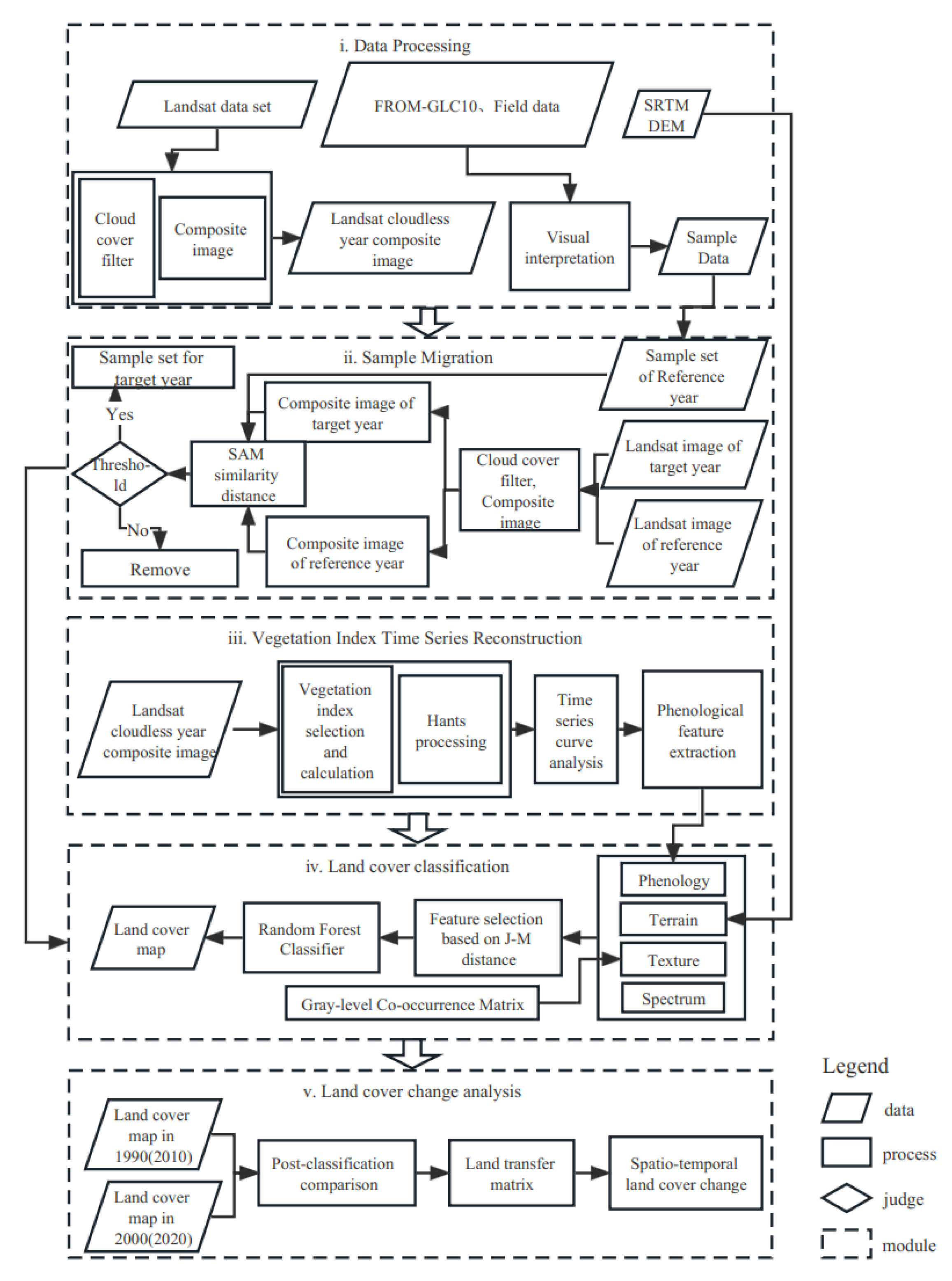
Figure 1.
Workflow of sample migration, phenological feature extraction, and land cover classification on the GEE.
Figure 1.
Workflow of sample migration, phenological feature extraction, and land cover classification on the GEE.
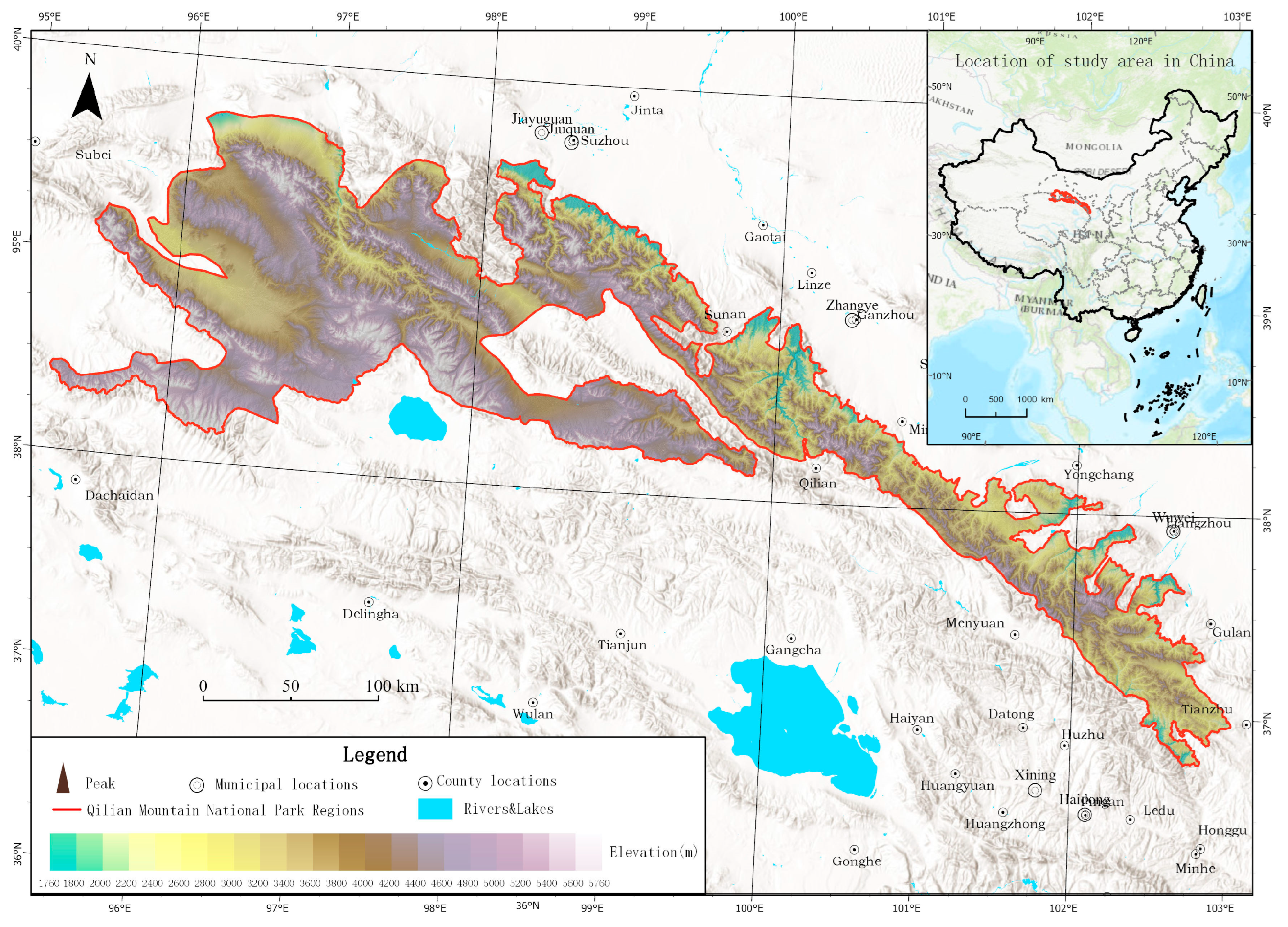
Figure 2.
Location of the Qilian Mountain National Park.
Figure 2.
Location of the Qilian Mountain National Park.
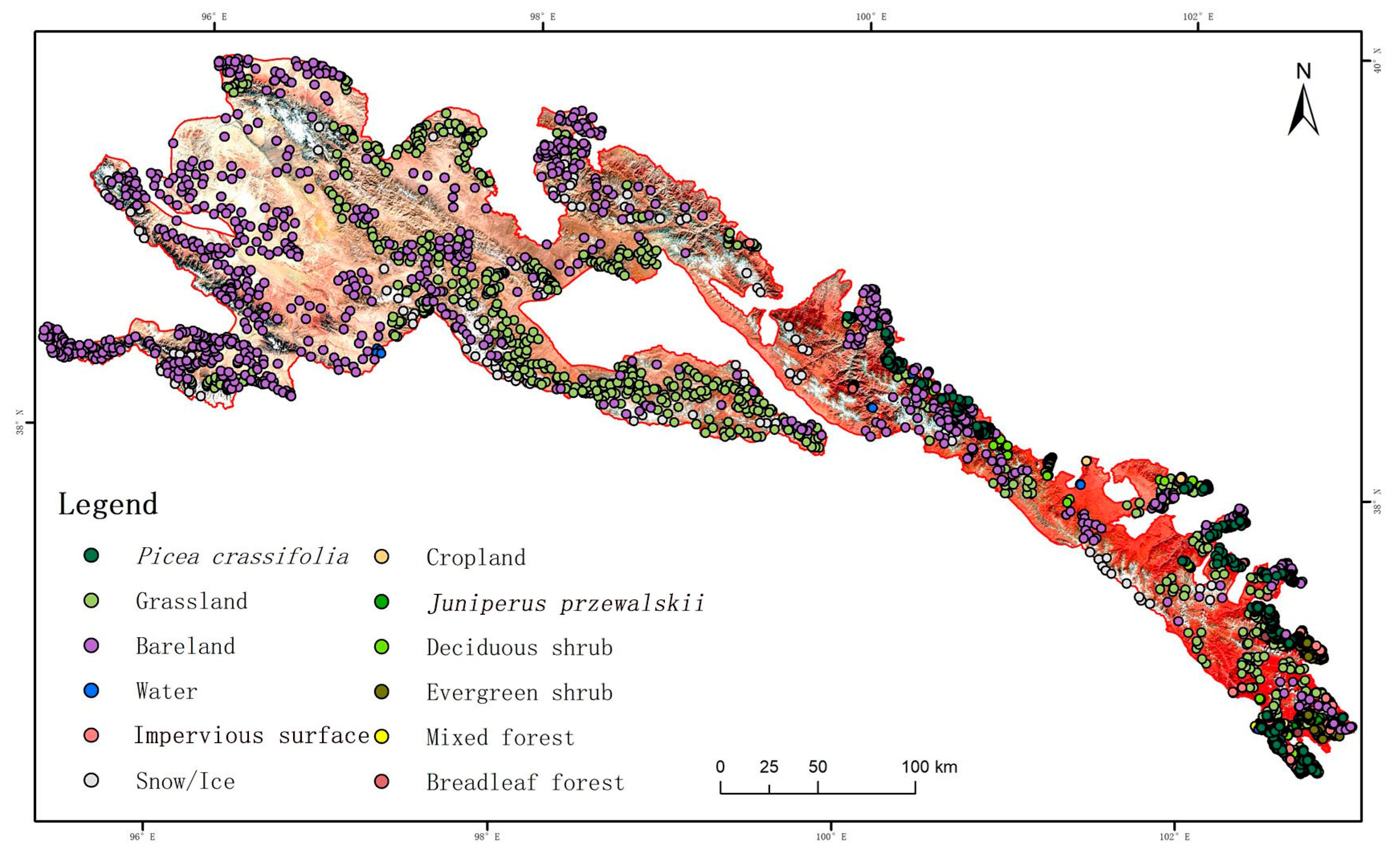
Figure 3.
Spatial distribution of samples in 2020.
Figure 3.
Spatial distribution of samples in 2020.
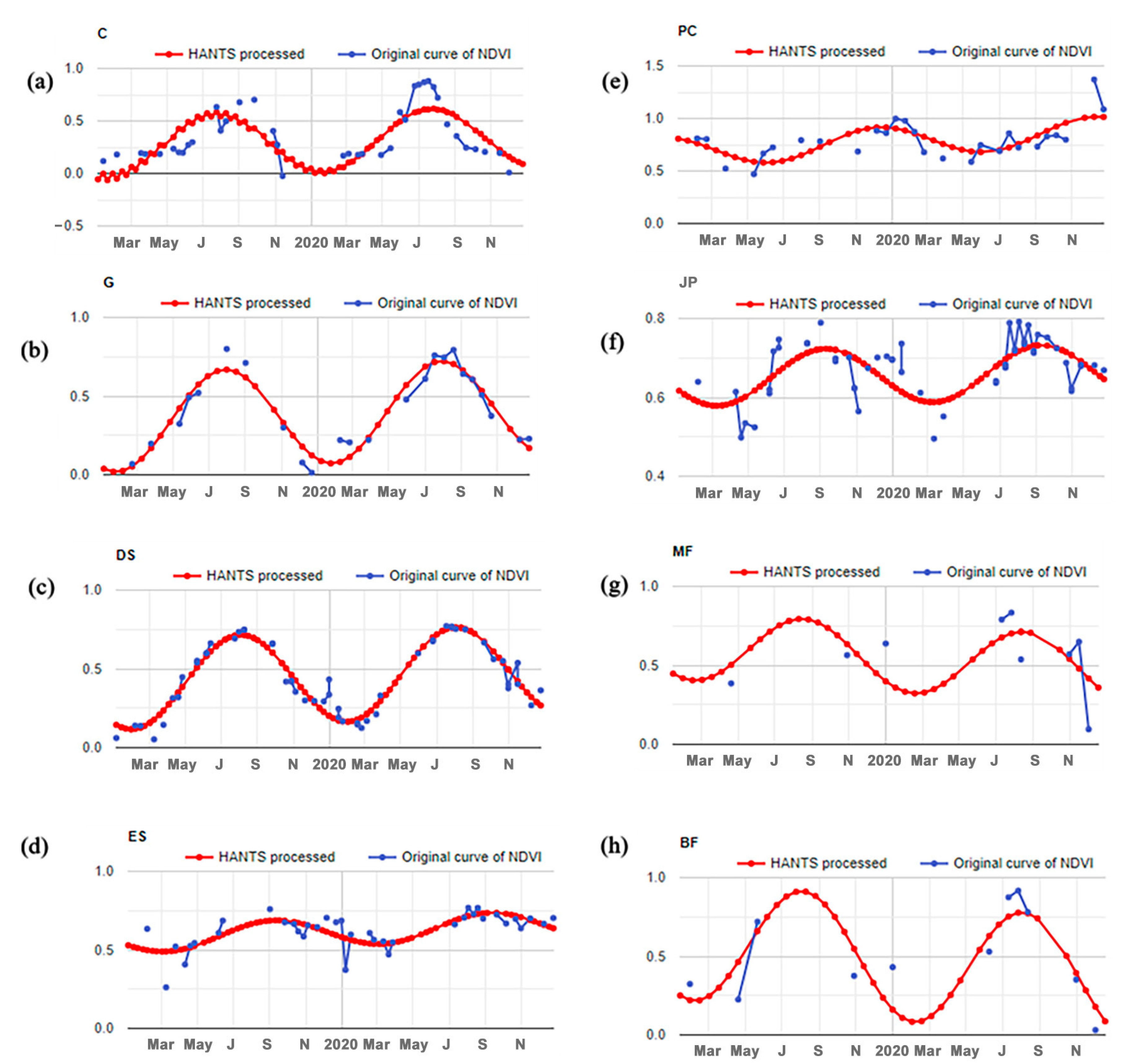
Figure 4.
Reconstruction of NDVI time series curves: (a) cropland, (b) grassland, (c) deciduous shrub, (d) evergreen shrub, (e) Picea crassifolia, (f) Juniperus przewalskii, (g) mixed forest, and (h) broadleaf forest (meaning of the letters on the X-axis from left to right: Mar, March; May, May; J, July; S, September; N, November).
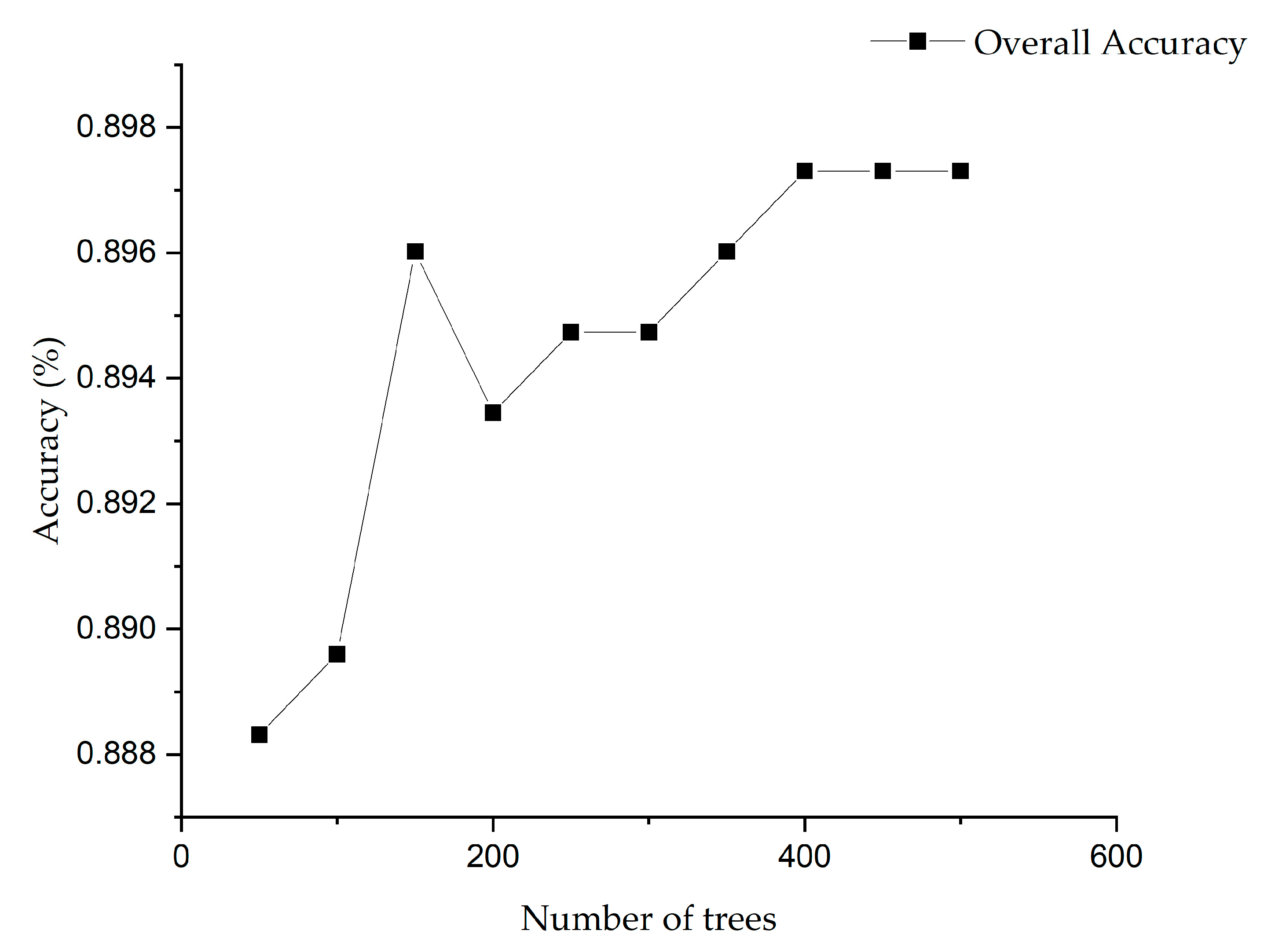
Figure 5.
Variation in land cover classification accuracy with the number of decision trees.
Figure 5.
Variation in land cover classification accuracy with the number of decision trees.
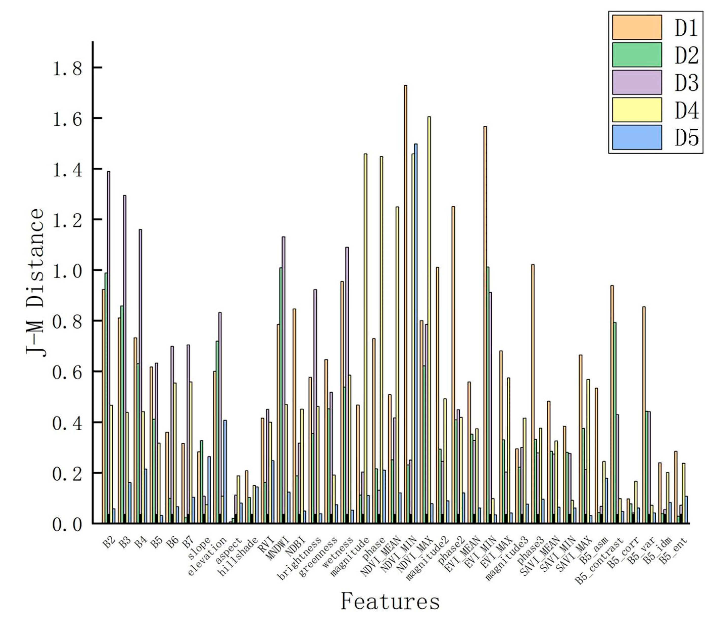
Figure 6.
The J-M distance between different land cover types of Landsat 8 in 2020 (D1 indicates IS and BL, D2 indicates C and G, D3 indicates DS and G, D4 indicates MF and PC, and D5 indicates BF and DS).
Figure 6.
The J-M distance between different land cover types of Landsat 8 in 2020 (D1 indicates IS and BL, D2 indicates C and G, D3 indicates DS and G, D4 indicates MF and PC, and D5 indicates BF and DS).
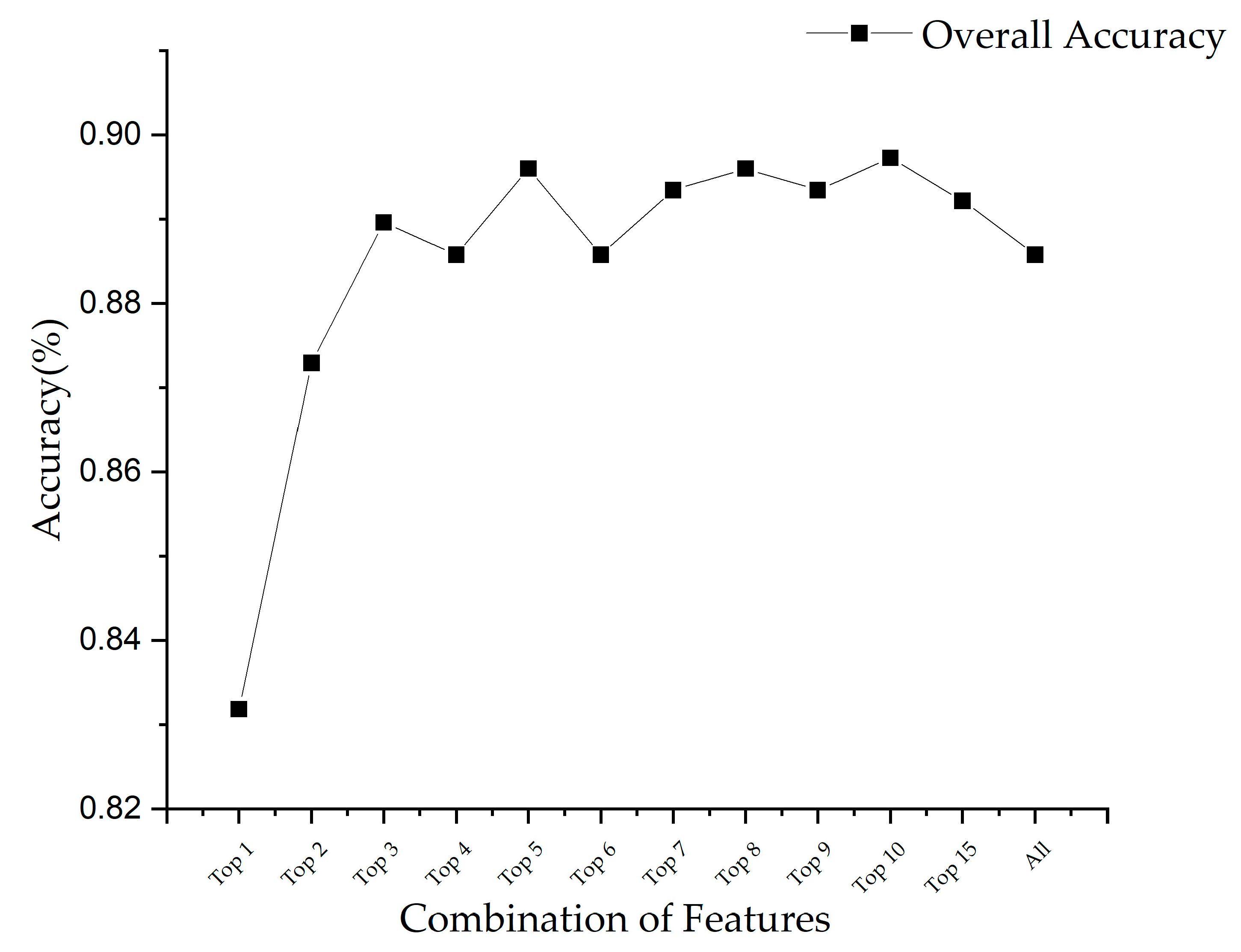
Figure 7.
Variation in land cover classification accuracy with feature combinations.
Figure 7.
Variation in land cover classification accuracy with feature combinations.
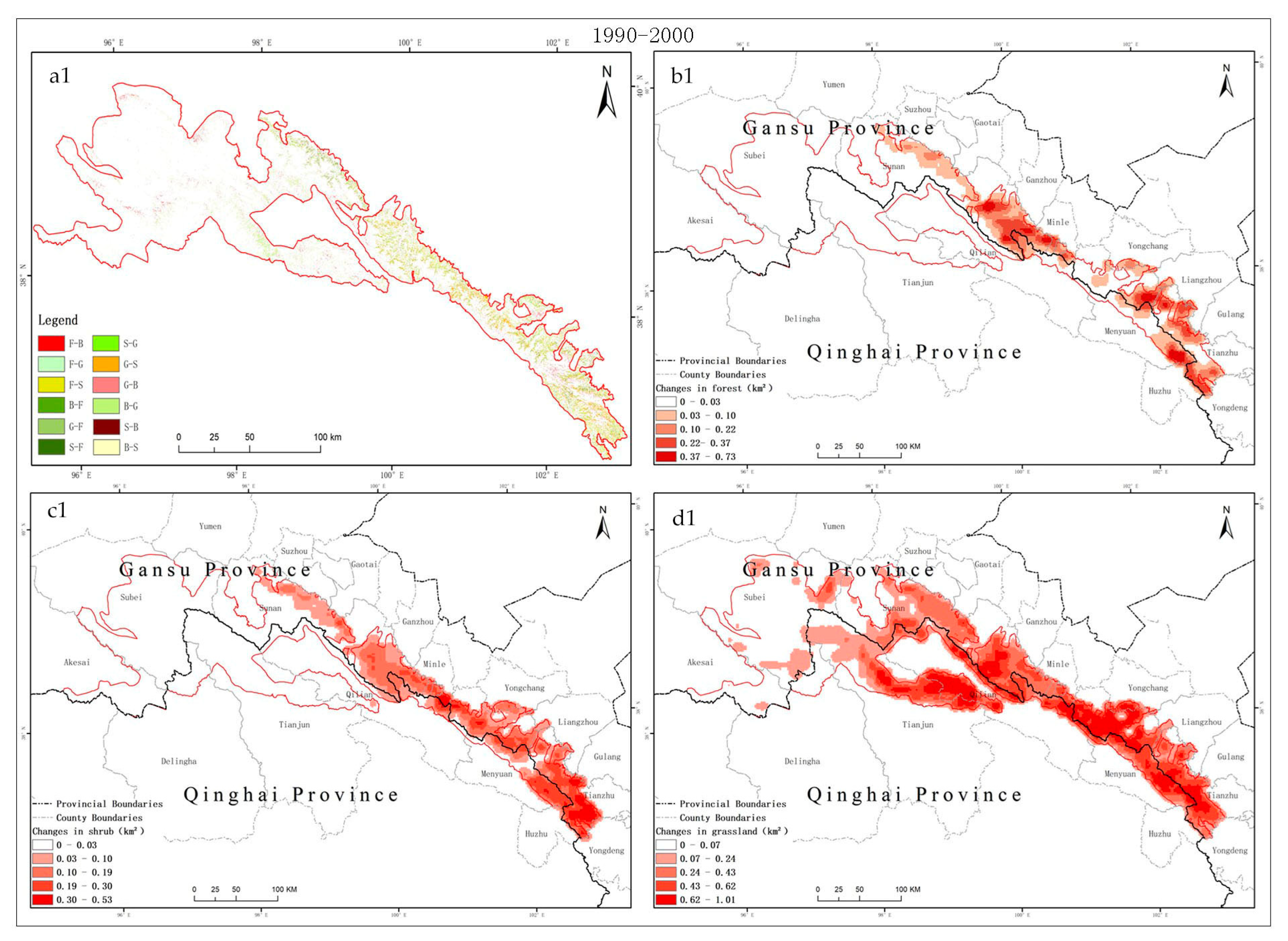
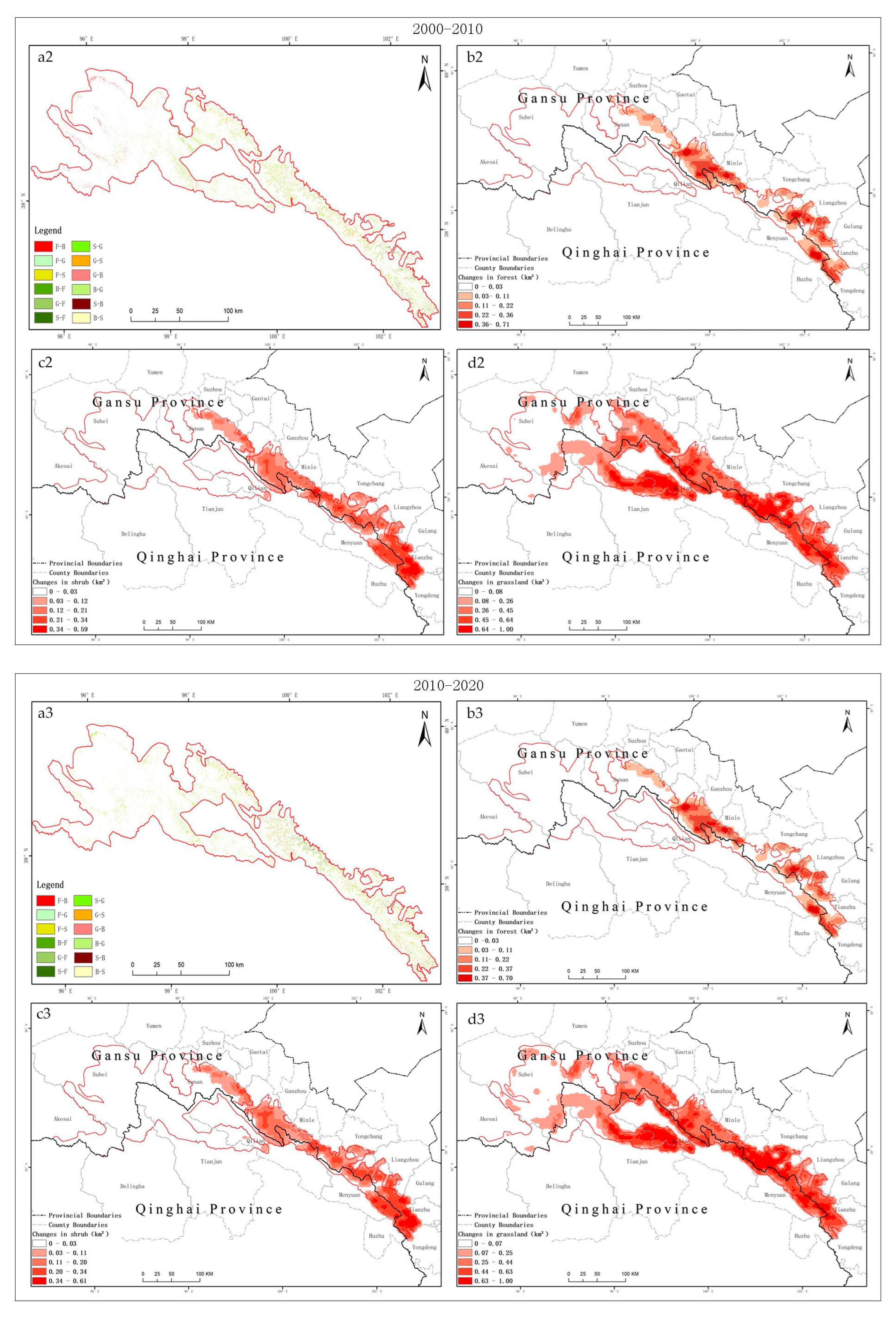
Figure 8.
Changes in each decade from 1990 to 2020: series (a1–a3) spatial distribution of forest, shrub and grassland changes; series (b1–b3), series (c1–c3), series (d1–d3) kernel density estimates of forest, shrub, and grassland area changes.
Figure 8.
Changes in each decade from 1990 to 2020: series (a1–a3) spatial distribution of forest, shrub and grassland changes; series (b1–b3), series (c1–c3), series (d1–d3) kernel density estimates of forest, shrub, and grassland area changes.
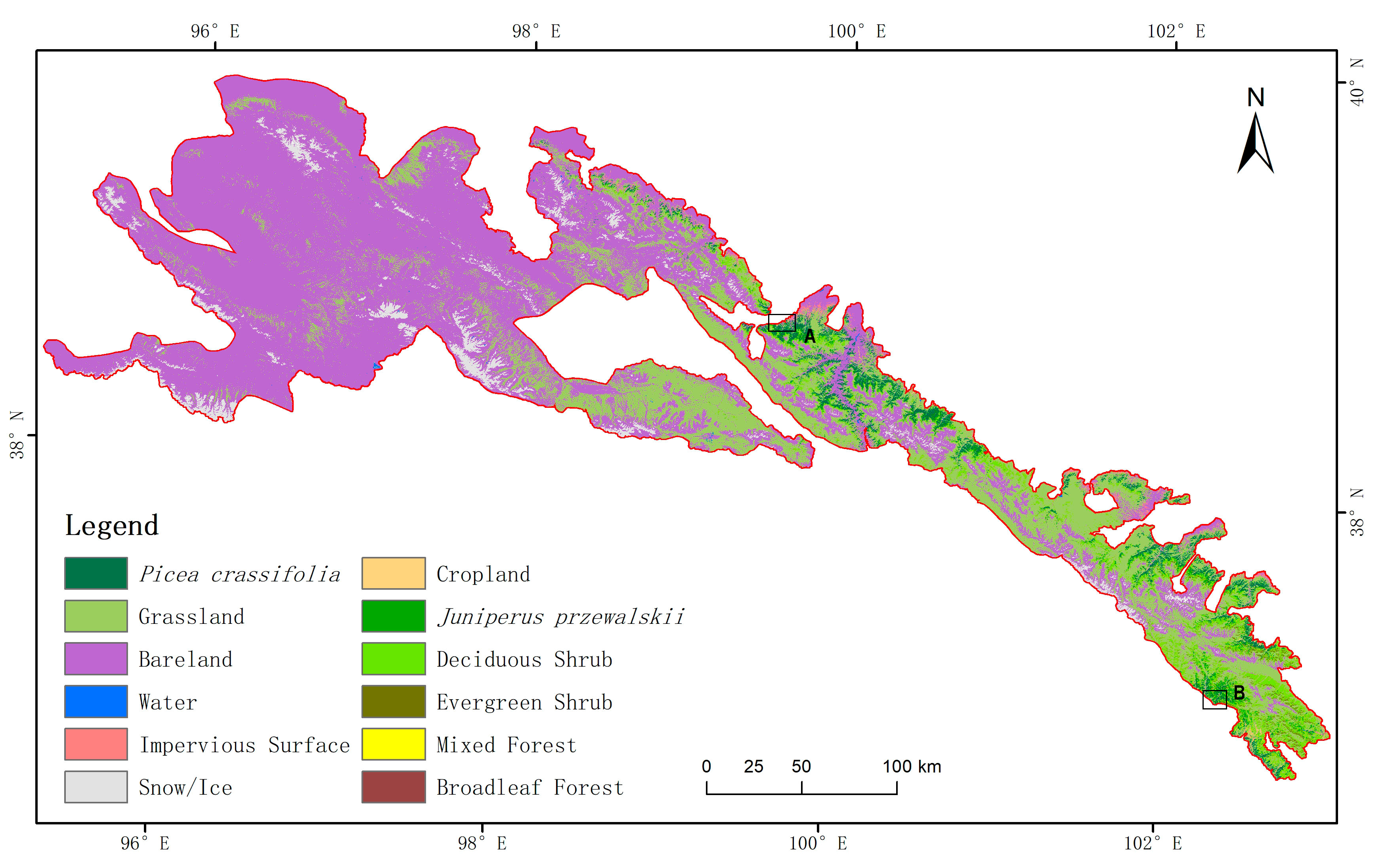
Figure 9.
Land cover classification result for 2020.
Figure 9.
Land cover classification result for 2020.
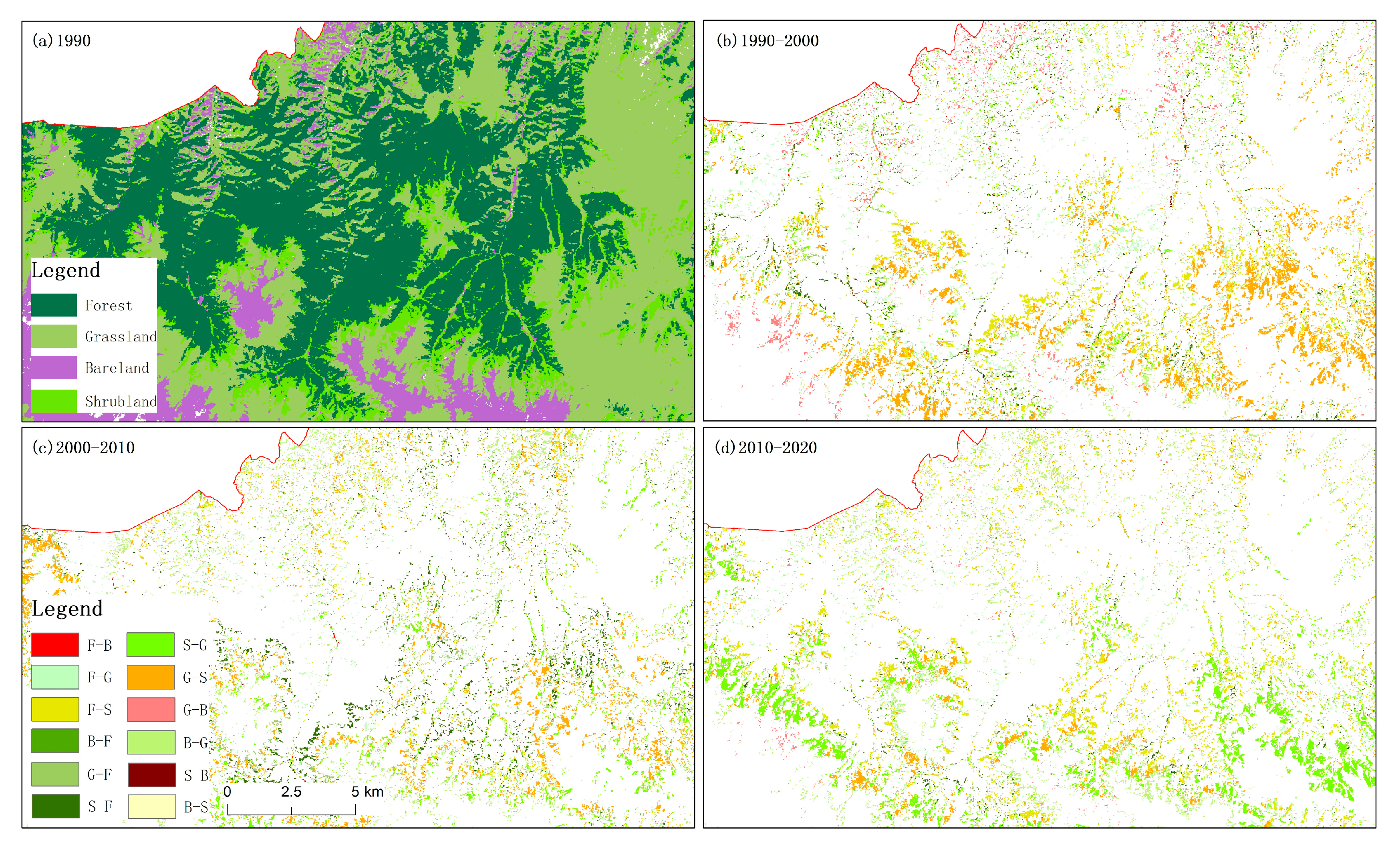
Figure 10.
Detailed map of forest, shrub, and grassland changes in Sunan county: (a) spatial distribution of forest, shrub, grassland and bare land in 1990; (b–d) the changes of spatial distribution of forest, shrub, grassland and bare land in 1990–2000, 2000–2010 and 2010–2020, respectively.
Figure 10.
Detailed map of forest, shrub, and grassland changes in Sunan county: (a) spatial distribution of forest, shrub, grassland and bare land in 1990; (b–d) the changes of spatial distribution of forest, shrub, grassland and bare land in 1990–2000, 2000–2010 and 2010–2020, respectively.
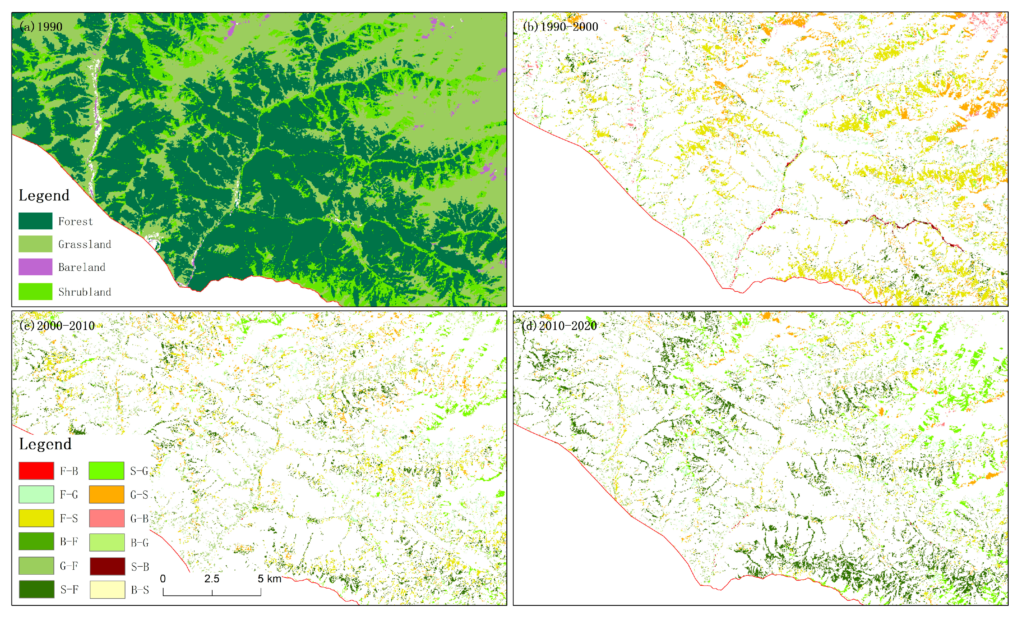
Figure 11.
Detailed map of forest, shrub, and grassland changes in Menyuan county: (a) spatial distribution of forest, shrub, grassland and bare land in 1990; (b–d) the changes of spatial distribution of forest, shrub, grassland and bare land in 1990–2000, 2000–2010 and 2010–2020, respectively.
Figure 11.
Detailed map of forest, shrub, and grassland changes in Menyuan county: (a) spatial distribution of forest, shrub, grassland and bare land in 1990; (b–d) the changes of spatial distribution of forest, shrub, grassland and bare land in 1990–2000, 2000–2010 and 2010–2020, respectively.
Table 1.
Interpretation signs of land cover.
Table 1.
Interpretation signs of land cover.
| First Class | Second Class | Third Class | Abbreviation | Description | Elevation Range |
|---|
| Forest | Evergreen Needleleaf Forest | Picea crassifolia | PC | Needle-leaved, evergreen; >85% of the forest is composed of Picea crassifolia, including plantations; H = 3–30 m | 2500–3600 m |
| Evergreen Needleleaf Forest | Juniperus przewalskii | JP | Needle-leaved, evergreen; >85% of the forest is composed of Juniperus przewalskii, including plantations | 2700–4000 m |
| Broadleaf Forest | Broadleaf Forest | BF | Flattened, broader, deciduous leaves; >85% broadleaf trees in the forest, including plantations | 1900–2700 m |
| Mixed Forest | Mixed Forest | MF | The respective proportions of coniferous and broad-leaved forests ranged from 25% to 75% and were above 3 m in height, including planted forests | 2500–2900 m |
| Shrubland | Evergreen Shrub | Evergreen Shrub | ES | Plant communities dominated by coniferous shrubs less than two meters in height | 3000–3700 m |
| Deciduous Shrub | Deciduous Shrub | DS | Plant communities dominated by deciduous shrubs less than two meters in height | 1900–3700 m |
| Grassland | Grassland | Grassland | G | Plant community dominated by annual or perennial herbaceous vegetation, including land in a managed state such as human grazing and harvesting | 1700–3000 m & 3500–4200 m |
| Agricultural Lands | Cropland | Cropland | C | Refers to land on which crops are grown | Below 2500 m |
| Impervious Surface | Impervious Surface | Impervious Surface | IS | Cities, towns, villages, and other settlements and roads, as well as artificial hard surfaces | Below 2500 m |
| Water | Water | Water | W | Including natural and artificially constructed relatively stationary water surfaces | - |
| Snow and Ice | Snow and Ice | Snow and Ice | SI | Land whose surface is covered by ice and snow year-round | Above 4600 m |
| Desert and Low-vegetated Lands | Desert and Bare soil | Bare Land | BL | Land with surface covered by soil and loose structure | 4200–4600 m |
Table 2.
Landsat image information.
Table 2.
Landsat image information.
| Year | Number of Images | Satellite | Date of Image Acquisition |
|---|
| 1990 | 509 | Landsat 5 TM | 1 January 1989–31 December 1990 |
| 2000 | 202 | Landsat 7 ETM+ | 1 January 1999–31 December 2000 |
| 2010 | 211 | Landsat 5 TM | 1 January 2009–31 December 2010 |
| 2020 | 666 | Landsat 8 OLI | 1 January 2019–31 December 2020 |
Table 3.
Image comparison of Picea crassifolia and Juniperus przewalskii.
Table 4.
Formulas of spectral indices.
Table 4.
Formulas of spectral indices.
| Spectral Index | Formula | Application |
|---|
| NDVI | | Mainly used to detect vegetation cover and distinguish vegetation from non-vegetation |
| EVI | | Good for detecting sparse vegetation |
| SAVI | | Reduces the effect of soil background and increases sensitivity to sparse vegetation |
| NDBI | | The value range is −1~1, and the value of artificial surfaces is greater than 0 |
| RVI | | A good reflection of the differences in vegetation growth status and coverage |
| MNDWI | | Good for distinguishing between water bodies and shadows |
Table 5.
The feature parameters selected to participate in the classification.
Table 5.
The feature parameters selected to participate in the classification.
| Type | Name | Parameters |
|---|
| Spectral | Landsat 5 and 7 bands | B1, B2, B3, B4, B5, B7 |
| Landsat 8 bands | B2, B3, B4, B5, B6, B7 |
| Tassel cap transformation | Brightness, greenness, wetness |
| Spectral index | MNDWI, NDBI, RVI |
| Phenological | NDVI_MIN, NDVI_MEAN, NDVI_MAX, magnitude, phase, EVI_MIN, EVI_MEAN, EVI_MAX, magnitude2, phase2, SAVI_MIN, SAVI_MEAN, SAVI_MAX, magnitude3, phase3 |
| Texture | Gray-level co-occurrence matrix (near-infrared) | B8(B5)_asm, B8(B5)_var, B8(B5)_idm, B8(B5)_ent, B8(B5)_contrast, B8(B5)_corr |
| Terrain | Terrain factors | SLOPE, ELEVATION, ASPECT, HILLSHADE |
Table 6.
Land cover samples in the study area based on sample migration.
Table 6.
Land cover samples in the study area based on sample migration.
| Year | 2020 | 2010 | 2000 | 1990 |
|---|
| Picea crassifolia | 476 | 475 | 475 | 440 |
| Grassland | 1081 | 971 | 972 | 931 |
| Bare land | 902 | 771 | 669 | 729 |
| Water body | 61 | 24 | 24 | 16 |
| Impervious surface | 242 | 242 | 236 | 235 |
| Snow and ice | 119 | 67 | 26 | 49 |
| Cropland | 247 | 231 | 224 | 228 |
| Juniperus przewalskii | 146 | 146 | 146 | 146 |
| Deciduous shrub | 287 | 280 | 279 | 248 |
| Evergreen shrub | 149 | 119 | 140 | 20 |
| Mixed forest | 63 | 54 | 54 | 45 |
| Broadleaf forest | 118 | 118 | 113 | 104 |
| Total | 3891 | 3498 | 3358 | 3191 |
Table 7.
Evaluation indices of accuracy.
Table 7.
Evaluation indices of accuracy.
| Name | Formula | Description |
|---|
| Overall Accuracy | | The number of correctly classified pixels divided by the total number of pixels |
| F1 Score |
| For a specific class A, TP is the number of pixels correctly classified as A, FP is the number of pixels incorrectly classified as A, FN is the number of pixels that A incorrectly classified as non-A, and TN is the number of pixels correctly classified as Non-A |
| User Accuracy | | For a specific class (A), UA is the number of pixels correctly classified as A divided by the total number of pixels in class A |
| Producer Accuracy | | For a specific class (A), PA is the number of pixels correctly classified as A divided by the number of all true pixels in class A |
Table 8.
Confusion matrix for 2020 classification results obtained from samples of all land cover (LC) types (the unit of the data in the table is number of samples).
Table 8.
Confusion matrix for 2020 classification results obtained from samples of all land cover (LC) types (the unit of the data in the table is number of samples).
| LC Type | PC | G | BL | W | IS | SI | C | JP | DS | ES | MF | BF |
|---|
| PC | 88 | 0 | 0 | 0 | 0 | 0 | 0 | 1 | 6 | 0 | 0 | 0 |
| G | 0 | 193 | 4 | 0 | 1 | 0 | 3 | 0 | 3 | 0 | 0 | 0 |
| BL | 0 | 3 | 174 | 0 | 2 | 0 | 0 | 0 | 0 | 0 | 0 | 0 |
| W | 0 | 0 | 0 | 13 | 0 | 0 | 0 | 0 | 0 | 0 | 0 | 0 |
| IS | 0 | 11 | 6 | 1 | 37 | 0 | 1 | 0 | 1 | 0 | 0 | 1 |
| SI | 0 | 0 | 2 | 0 | 0 | 25 | 0 | 0 | 0 | 0 | 0 | 0 |
| C | 0 | 11 | 0 | 0 | 1 | 0 | 38 | 0 | 1 | 0 | 0 | 2 |
| JP | 0 | 1 | 0 | 0 | 0 | 0 | 0 | 15 | 0 | 0 | 0 | 0 |
| DS | 0 | 8 | 0 | 0 | 0 | 0 | 2 | 0 | 44 | 1 | 0 | 0 |
| ES | 2 | 0 | 0 | 0 | 0 | 0 | 0 | 0 | 0 | 39 | 0 | 0 |
| MF | 3 | 0 | 0 | 0 | 0 | 0 | 0 | 1 | 0 | 0 | 12 | 0 |
| BF | 1 | 2 | 1 | 0 | 0 | 0 | 2 | 0 | 4 | 0 | 0 | 12 |
Table 9.
Classification features for 2020.
Table 9.
Classification features for 2020.
| Combination | Features |
|---|
| Top 1 | NDVI_MIN, EVI_MIN, B2, NDVI_MAX, NDBI, MNDWI |
| Top 2 | Top 1 + ELEVATION, B3 |
| Top 3 | Top 2 + phase2, B4, magnitude, SLOPE |
| Top 4 | Top 3 + RVI, phase, phase3 |
| Top 5 | Top 4 + magnitude2, B8_contrast, wetness, NDVI_MEAN |
| Top 6 | Top 5 + brightness |
| Top 7 | Top 6 + B8_asm, EVI_MAX |
| Top 8 | Top 7 + SAVI_MAX |
| Top 9 | Top 8 + B7, B8_var, HILLSHADE |
| Top 10 | Top 9 + B6, greenness |
| Top 15 | Top 10 + B5, B8_ent |
Table 10.
Final classification features.
Table 10.
Final classification features.
| Dataset | Combination | Number | Name |
|---|
| Landsat 8 | Top 10 | 28 | NDVI_MIN, EVI_MIN, B2, NDVI_MAX, NDBI, MNDWI, ELEVATION, B3, phase2, B4, magnitude, SLOPE, RVI, phase, phase3, magnitude2, B8_contrast, wetness, NDVI_MEAN, brightness, B8_asm, EVI_MAX, SAVI_MAX, B7, B8_var, HILLSHADE, B6, greenness |
Table 11.
Land transfer matrix for 1990–2000 (km2).
Table 11.
Land transfer matrix for 1990–2000 (km2).
| | F | G | BL | W | IS | SI | C | S | Total Area in 2000 |
|---|
| F | 1520.2 | 73.0 | 54.3 | 2.7 | 1.7 | 0.0 | 0.6 | 190.1 | 1842.6 |
| G | 107.5 | 11,002.2 | 914.8 | 3.8 | 42.4 | 17.5 | 11.0 | 263.7 | 12,363.0 |
| BL | 6.3 | 904.4 | 29,951.5 | 69.6 | 16.1 | 381.2 | 3.9 | 16.8 | 31,349.8 |
| W | 0.5 | 0.9 | 164.2 | 21.2 | 0.1 | 3.1 | 0.0 | 0.4 | 190.4 |
| IS | 5.5 | 254.3 | 58.3 | 0.5 | 37.3 | 0.0 | 6.7 | 20.9 | 383.5 |
| SI | 0.0 | 42.1 | 277.0 | 1.2 | 0.0 | 1562.4 | 0.0 | 0.0 | 1882.7 |
| C | 0.5 | 8.9 | 2.0 | 0.0 | 4.1 | 0.0 | 26.9 | 2.8 | 45.2 |
| S | 286.2 | 572.8 | 43.1 | 4.2 | 3.1 | 0.1 | 1.7 | 1231.7 | 2142.8 |
| Total area in 1990 | 1926.6 | 12,858.5 | 31,465.3 | 103.2 | 104.6 | 1964.4 | 50.8 | 1726.5 | 50,200.0 |
Table 12.
Transfer matrix of land cover for 2000–2010 (km2).
Table 12.
Transfer matrix of land cover for 2000–2010 (km2).
| | F | G | BL | W | IS | SI | C | S | Total Area in 2010 |
|---|
| F | 1489.8 | 137.8 | 8.9 | 1.4 | 5.4 | 0.0 | 0.7 | 215.2 | 1859.3 |
| G | 60.8 | 11,324.1 | 1623.7 | 2.2 | 238.7 | 53.1 | 13.2 | 374.5 | 13,690.2 |
| BL | 13.9 | 392.7 | 29,263.6 | 163.1 | 20.8 | 437.3 | 0.5 | 11.1 | 30,303.0 |
| W | 2.4 | 2.4 | 26.2 | 15.5 | 0.8 | 2.8 | 0.1 | 2.0 | 52.1 |
| IS | 14.1 | 86.9 | 97.7 | 1.0 | 98.1 | 0.0 | 6.9 | 26.6 | 331.3 |
| SI | 0.0 | 7.3 | 318.7 | 6.6 | 0.0 | 1389.5 | 0.0 | 0.0 | 1722.2 |
| C | 0.5 | 8.3 | 1.2 | 0.0 | 5.3 | 0.0 | 21.3 | 2.5 | 39.1 |
| S | 261.1 | 403.4 | 9.7 | 0.6 | 14.3 | 0.0 | 2.6 | 1510.8 | 2202.7 |
| Total area in 2000 | 1842.6 | 12,363.0 | 31,349.8 | 190.4 | 383.5 | 1882.7 | 45.2 | 2142.8 | 50,200.0 |
Table 13.
Land transfer matrix for 2010–2020 (km2).
Table 13.
Land transfer matrix for 2010–2020 (km2).
| | F | G | BL | W | IS | SI | C | S | Total Area in 2020 |
|---|
| F | 1549.6 | 54.7 | 31.5 | 1.2 | 17.6 | 0.0 | 2.6 | 207.4 | 1864.4 |
| G | 84.1 | 11,007.5 | 437.1 | 3.9 | 98.2 | 21.0 | 15.6 | 396.3 | 12,063.8 |
| BL | 25.2 | 1917.1 | 29,198.7 | 32.4 | 68.2 | 164.4 | 0.6 | 21.5 | 31,428.0 |
| W | 0.8 | 0.7 | 26.4 | 9.8 | 1.7 | 3.8 | 0.0 | 0.2 | 43.4 |
| IS | 10.5 | 294.4 | 91.4 | 0.5 | 126.6 | 0.0 | 4.7 | 13.5 | 541.7 |
| SI | 0.0 | 5.0 | 517.2 | 4.0 | 0.0 | 1533.0 | 0.0 | 0.0 | 2059.2 |
| C | 2.0 | 8.5 | 0.0 | 0.0 | 3.0 | 0.0 | 14.2 | 2.4 | 30.1 |
| S | 187.1 | 402.1 | 0.8 | 0.3 | 16.1 | 0.0 | 1.6 | 1561.3 | 2169.4 |
| Total area in 2010 | 1859.3 | 13,690.2 | 30,303.0 | 52.1 | 331.3 | 1722.2 | 39.1 | 2202.7 | 50,200.0 |
Table 14.
Accuracy evaluation of land cover classification results.
Table 14.
Accuracy evaluation of land cover classification results.
| Type | 1990 | 2000 | 2010 | 2020 |
|---|
| PA (%) | UA (%) | Error | F1 Score | PA (%) | UA (%) | Error | F1 Score | PA (%) | UA (%) | Error | F1 Score | PA(%) | UA (%) | Error | F1 Score |
|---|
| PC | 0.900 | 0.914 | −0.014 | 0.907 | 0.914 | 0.932 | −0.018 | 0.923 | 0.938 | 0.930 | 0.008 | 0.934 | 0.937 | 0.953 | −0.016 | 0.945 |
| G | 0.845 | 0.932 | −0.087 | 0.886 | 0.869 | 0.945 | −0.076 | 0.905 | 0.879 | 0.946 | −0.067 | 0.911 | 0.894 | 0.946 | −0.052 | 0.919 |
| BL | 0.944 | 0.949 | −0.005 | 0.946 | 0.959 | 0.946 | 0.013 | 0.952 | 0.960 | 0.963 | −0.003 | 0.961 | 0.947 | 0.963 | −0.016 | 0.955 |
| W | 0.953 | 0.965 | −0.012 | 0.959 | 0.967 | 0.942 | 0.025 | 0.954 | 0.900 | 0.937 | −0.037 | 0.918 | 0.976 | 0.976 | 0 | 0.976 |
| IS | 0.812 | 0.823 | −0.011 | 0.817 | 0.790 | 0.789 | 0.001 | 0.789 | 0.793 | 0.815 | −0.022 | 0.804 | 0.861 | 0.833 | 0.028 | 0.847 |
| SI | 0.861 | 0.884 | −0.023 | 0.872 | 0.984 | 0.969 | 0.015 | 0.976 | 0.967 | 0.896 | 0.071 | 0.930 | 0.962 | 0.907 | 0.055 | 0.934 |
| C | 0.824 | 0.808 | 0.016 | 0.816 | 0.819 | 0.848 | −0.029 | 0.833 | 0.853 | 0.859 | −0.006 | 0.856 | 0.798 | 0.804 | −0.006 | 0.801 |
| JP | 0.898 | 0.850 | 0.048 | 0.873 | 0.874 | 0.844 | 0.03 | 0.859 | 0.908 | 0.903 | 0.005 | 0.905 | 0.935 | 0.941 | −0.006 | 0.938 |
| DS | 0.802 | 0.798 | 0.004 | 0.800 | 0.820 | 0.785 | 0.035 | 0.802 | 0.779 | 0.813 | −0.034 | 0.796 | 0.800 | 0.866 | −0.066 | 0.832 |
| ES | 0.834 | 0.825 | 0.009 | 0.829 | 0.810 | 0.874 | −0.064 | 0.841 | 0.842 | 0.903 | −0.061 | 0.871 | 0.892 | 0.926 | −0.034 | 0.909 |
| MF | 0.786 | 0.797 | −0.011 | 0.791 | 0.771 | 0.786 | −0.015 | 0.778 | 0.780 | 0.801 | −0.021 | 0.790 | 0.813 | 0.825 | −0.012 | 0.819 |
| BF | 0.814 | 0.803 | 0.011 | 0.808 | 0.805 | 0.815 | −0.01 | 0.810 | 0.831 | 0.826 | 0.005 | 0.828 | 0.806 | 0.801 | 0.005 | 0.803 |
| OA(%) | 0.839 | 0.860 | 0.880 | 0.897 |


