HTDet: A Hybrid Transformer-Based Approach for Underwater Small Object Detection

Abstract

As marine observation technology develops rapidly, underwater optical image object detection is beginning to occupy an important role in many tasks, such as naval coastal defense tasks, aquaculture, etc. However, in the complex marine environment, the images captured by an optical imaging system are usually severely degraded. Therefore, how to detect objects accurately and quickly under such conditions is a critical problem that needs to be solved. In this manuscript, a novel framework for underwater object detection based on a hybrid transformer network is proposed. First, a lightweight hybrid transformer-based network is presented that can extract global contextual information. Second, a fine-grained feature pyramid network is used to overcome the issues of feeble signal disappearance. Third, the test-time-augmentation method is applied for inference without introducing additional parameters. Extensive experiments have shown that the approach we have proposed is able to detect feeble and small objects in an efficient and effective way. Furthermore, our model significantly outperforms the latest advanced detectors with respect to both the number of parameters and the mAP by a considerable margin. Specifically, our detector outperforms the baseline model by 6.3 points, and the model parameters are reduced by 28.5 M.

1. Introduction

Over the past few years, the technology used to detect underwater objects has become increasingly widely used, for example, in tasks such as underwater ecological monitoring, underwater pipeline maintenance, and wreck fishing [1,2,3,4,5,6]. Mainstream methods for underwater object detection fall into two main types: optical imaging and sonar. However, the optical image detection method has significant advantages in underwater object detection tasks at close range, as an optical image has a high resolution and good flexibility. However, unlike object detection in natural images, optical underwater imaging is affected by scattering and absorption of water bodies, which would produce images with more severe degradation [7,8]. As a result, underwater images have the following characteristics: low contrast, non-uniform illumination, and blurring, due to various complex environments. More specifically, object size in the image is usually less than $32\times 32$ pixels, and the object signal-to-noise ratio (SNR) is much lower than −3 dB; we refer to this as the feeble and small object, as shown in Figure 1. As a result, the task of optical underwater object detection with feeble and small objects is challenging. The main challenges for small object detection are low object resolution, complex backgrounds, insignificant features, and limited contextual information. This is usually combined with a low signal-to-noise ratio, which means that the object signal is very easily overwhelmed by the background signal. Moreover, the existing general purposed object detection algorithms have limited accuracy when directly applied to underwater object detection, and how to detect the object efficiently and effectively within a challenging underwater environment is an urgent task to be solved.

Recent research into optical imaging technologies for underwater object detection has seen rapid development. Wang et al. presented a logical stochastic resonance-based approach for detection of feeble objects [9]. There are also some scholars who have done more work on underwater optical image detection applications [6,10,11]. However, they did not thoroughly study the issues of feeble and small object detection underwater, and this area of research still suffers from the following problems.

First, global context information such as object shape, contour, etc., plays an important role in underwater optical image object detection, especially feeble and small object detection, and existing convolutional neural network (CNN) based detectors are not well equipped to extract such long-range relationships. Second, generic detectors usually contain significant numbers of parameters and are therefore not suitable for underwater optical image object detection applications in real time. Third, feature enhancement is usually introduced by feature pyramid networks (FPNs) in existing models of underwater optical image object detection. However, typical FPNs only use neighbor fusion to gradually enhance the object signal, and when the situation involves a feeble and small object, the object signal will be overwhelmed by other signals as the fusion steps increase one by one, resulting in the feeble and small object signal vanishing problem.

To solve the first two noted problems, we introduce a hybrid lightweight network based on transformers to provide a robust global context representation of objects, especially feeble and small objects. In addition, the proposed lightweight backbone has fewer parameters. It has been proved that the transformer is superior to CNNs for modeling long-range relationships, but the transformer requires a larger amount of training data and has significantly higher computational complexity than CNNs. Underwater optical images are often expensive to obtain, which makes it hard to apply the transformer directly to diverse applications of underwater optical images. In contrast, the hybrid architecture contains both CNN and transformer structures. The CNN structure in the hybrid network brings a certain inductive bias, thus reducing the need for data. Then, the hybrid network can model long-range relationships effectively and efficiently while maintaining comparatively lower computational complexity than transformers. As a result, the procedure requires as few data and training time as a CNN and performs much better than CNN.

Furthermore, to solve the feeble and small object signal vanishing problem, we propose a novel feeble-object-friendly module referred to as the fine-grained feature pyramid network (fine-grained FPN). In the fine-grained FPN, cumulative bridges between different layers are designed to enhance the feeble and small object signals so that the feeble and small object signal vanishing problem can be eliminated.

Finally, a memory cost-free approach is introduced, called test-time-augmentation [12] (TTA), to further improve our detector’s performance.

On the basis of the above points, a novel lightweight hybrid transformer-based underwater detector is proposed for the detection of underwater optical images of feeble and small objects. A schematic diagram of our proposed algorithm is shown in Figure 2. The image is first expanded through a series of transformations and then extracted into the basic features by the hybrid backbone network, and then further signal enhancement is realized by a fine-grained feature pyramid network to obtain the final features for detection. TTA is then used to further improve the detection accuracy and obtain the final detection results. The entire detector has a remarkably small number of parameters and can be used in applications where real-time detection of underwater optical images is required. The major difference between our approach and previous ones is that we propose a novel efficient solution to the feeble object detection problem based on the transformer hybrid network. We experimentally validate our detector and verify the significant superiority of our detector over several advanced detectors, and we further investigate the effectiveness of each part of our detector.

Consequently, the contributions are listed below:

• A novel transformer-based hybrid detector for underwater feeble and small object detection is proposed, which can extract the global and local context information efficiently and effectively;
• To tackle the signal vanishing problem of feeble and small objects, fine-grained (FPN) is designed to cumulatively fuse low-level and high-level features;
• To further enhance the detector’s accuracy, we use the memory-free TTA approach for real-time detection.

The remainder of the paper is structured in the following way. In Section 2, a brief review of underwater object detection is given. Section 3 presents the details of each component. In Section 4, we validate the superiority of our detector and the effectiveness of each component of our detector. Additionally, we conducted a robustness analysis of our model in the presence of various noise disturbances. Section 5 is a discussion of the shortcomings of the current research methodology and the main directions for future research. Finally, in Section 6, we give a brief conclusion to our work in this paper.

2. Related Work

2.1. General Purpose Object Detection

General object detection algorithms started with classical algorithms such as faster RCNN [13], YOLOv1 [14], etc. Faster RCNN was the first practical two-stage detection algorithm, and YOLO was the first object detection algorithm that could detect in real-time in practice. In order to better detect small targets, SSD [15] was proposed. Subsequently, RetinaNet [16] was proposed to address the sample imbalance problem of the single-stage algorithm, allowing the performance of the single-stage algorithm to match that of the two-stage algorithm for the first time while maintaining the same speed of detection. With the popularity of the transformer in the field of computer vision, some scholars proposed the transformer-based object detection algorithms Detr [17] and Deformable Detr [18], which can achieve the performance of faster RCNN, but with a long training period, high cost, and a huge number of model parameters. In order to further obtain better detection results, many scholars have designed more balanced sample allocation methods, such as ATSS [19] and AutoAssign [20]; some other scholars have tried to design more efficient detection algorithms, such as YOLOv3 [21] and YOLOv4 [22]; some other scholars have studied the feature fusion and proposed methods such as S-FPN [23]. Generic object detection algorithms are used in a variety of fields in addition to object perception in common scenarios [24,25]. For example, in remote sensing, general object detection algorithms are used for object perception and detection in optical and SAR images [26,27,28]. Wu et al. proposed the ORSIm detector, which uses multiple methods to enhance object detection in remote sensing images [29]. UIU-Net developed a multi-scale detection algorithm for small infrared objects, with promising performance [30]. Generic object detection algorithms are widely used in underwater optical sensing [31,32]. Numerous methods have been introduced into the object detection algorithm to improve the detection of the model [33], but there is still room to promote the model.

Despite the rapid development of general purpose object detection, these methods are unable to be directly applied to underwater optical image object detection due to the severe noise in underwater images. It is an urgent problem to improve these methods for feeble object detection in a high-noise environment.

2.2. Underwater Object Detection

Underwater optical images typically contain many feeble and small objects scattered and absorbed by the water column. It is hard to detect feeble and small objects with low SNRs in underwater optical images. To overcome this problem, Zhao et al. [34] presented a composed backbone with an enhanced pathway aggregation network, which strengthened the representation of the object in the image. Their work achieved favorable results on underwater optical images, but the composed backbones were designed with a large number of parameters and were not suitable for real-time applications. Zhang et al. [11] proposed a YOLOv4 [22] based lightweight underwater detector, which used MobileNetv2 [35] and depth-wise separable convolution [36] to reduce the parameters in the network. This work obtained relatively better results compared to traditional detectors; nevertheless, CNN was still the backbone of the detector, thus it was difficult to extract the global representation of the object in a robust way. To solve the above issues, we exploit the advantages of transformer and CNN to extract the global context information of feeble and small objects. Further, the low-level feature is strengthened to get a fine-grained representation of feeble and small objects, which helps to detect the object with low SNRs in underwater images.

2.3. Lightweight Detectors

Lightweight detectors have received a great deal of attention in the last few years. Wang et al. [6] proposed a lightweight underwater detector, RLOD, based on the hourglass network. RLOD introduced dense connections and FPN [37] to boost model performance, and it could get 11.11 frames per second speed on the NVIDIA Jetson TX2 platform. Yeh et al. [38] presented a joint learning scheme both for underwater detection and color conversion, which could handle two tasks with fewer parameters. Their network was implemented on a Raspberry Pi platform for underwater object detection and achieved comparatively favorable results. Tan et al. [39] proposed a lightweight underwater detector FL-YOLOV3-TINY based on YOLOv3-Tiny and Mobilenet [35], which yielded better real-time performance and higher AP performance compared to baselines.

All these lightweight models above have achieved relatively remarkable performance; however, pure CNNs were still used as their base architectures, and CNNs specialize in modeling local relationships and are not effective in modeling global relationships. To better exploit the global context information of feeble and small objects in real-time underwater optical image applications, we proposed a lightweight underwater optical image detector based on hybrid backbone to achieve better extraction of global context information of objects while improving the detection performance of feeble objects.

3. Method

A major drawback of underwater object detection networks is their large parameter overhead. In addition, feeble and small objects with low SNR are another challenging issue in this field. We exploit both the advantages of the lightweight backbone and the transformer’s capability of extracting the global context information of the objects to propose an efficient detector for underwater optical image feeble and small object detection. In addition to layer-specific global context information, global context information oriented to multi-layer fusion is equally important for small and feeble object detection, thus, a novel cumulative bridge module is required.

3.1. Overall Architecture

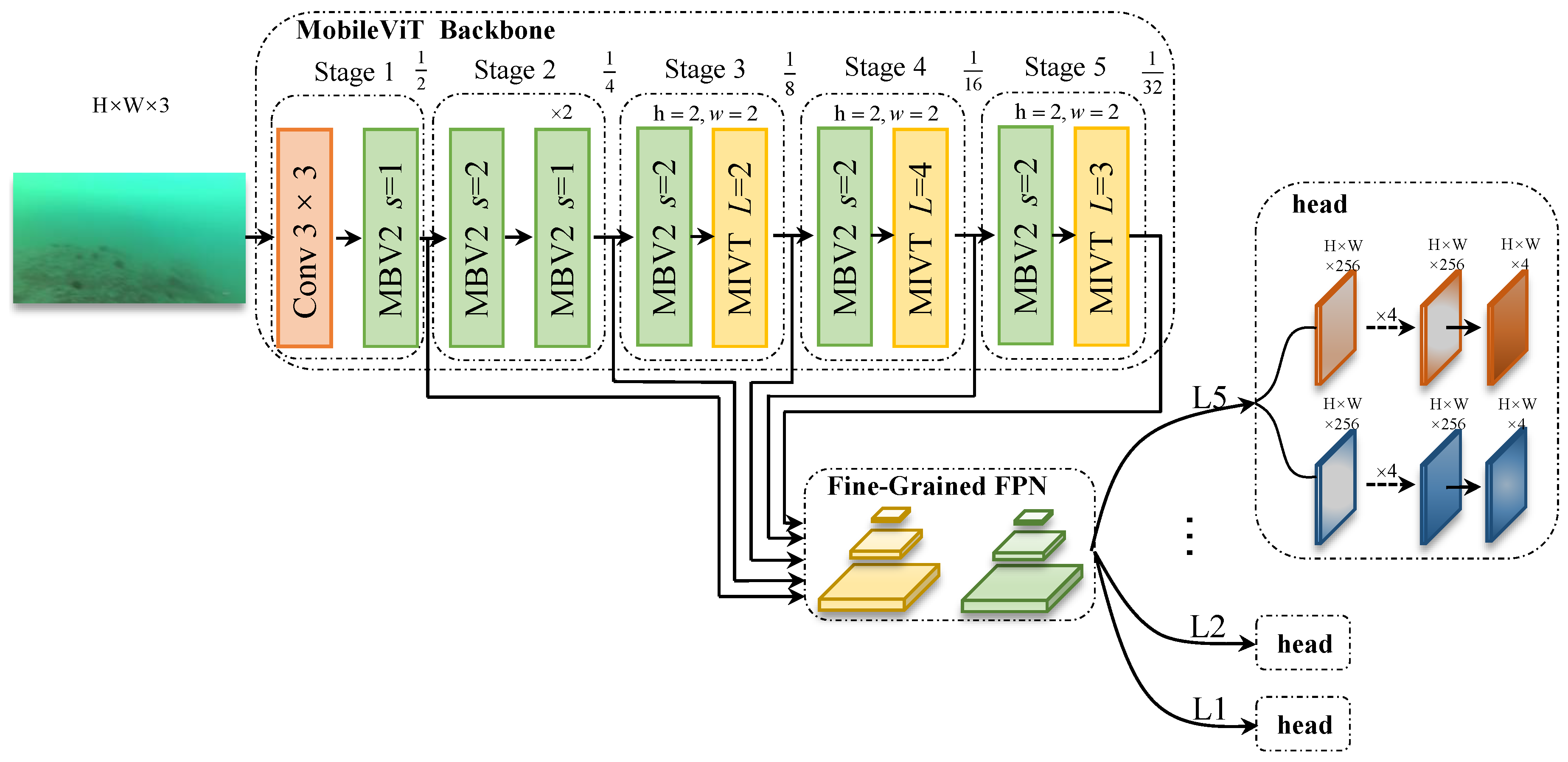
Our proposed model is outlined in Figure 3. The whole model consists of three parts.

The first component is the lightweight transformer-based hybrid backbone–MobileViT [40]. The backbone is composed of three main blocks. The first one is the MobileNetV2 block [35] with stride 2 (MBV2 with $s=2$ in Figure 3). The second one is the MobileNetV2 block with stride 1 (MBV2 with $s=1$ in Figure 3), and the last one is the MobileViT block (MVIT in Figure 3), which is the main difference from the local dependent aware model. For a given input image of shape $H\times W\times 3$, the first stage downsamples the image via a convolution layer using a $3\times 3$ kernel with a stride of 2. Subsequently, a block of MBV2 with a stride 1 is employed to extract the features having the same size as its input. For the following stages, MBV2 blocks with stride 2 are used as down-sampling blocks, and MVIT blocks are used as feature extractors, except for stage 2, which uses an MBV2 block with stride 1 as its feature extractor.

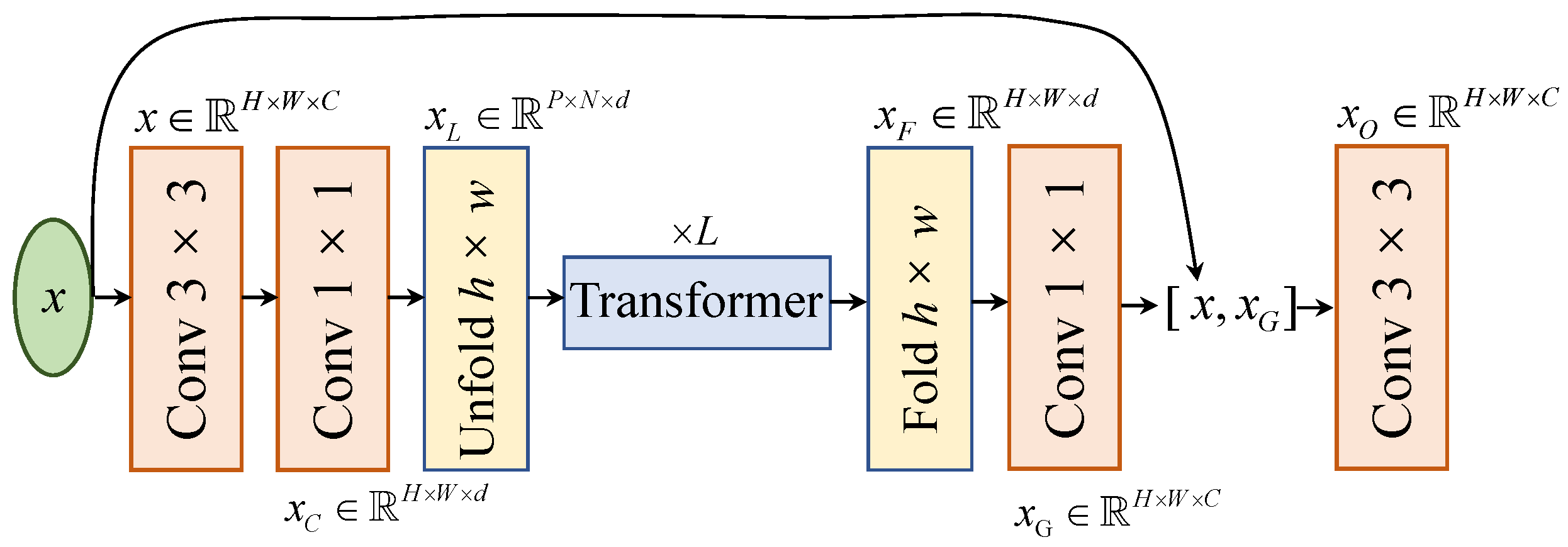
The transformer is a flexible solution for encoding the global context information of objects in images; however, pure transformer-based networks usually bring a huge computational footprint. Hybrid transformer-based networks, on the other hand, can benefit from a lightweight network with less computation and the ability to encode global-dependent contextual information. The MVIT block is a subnetwork that can be successfully inserted into a lightweight CNN to form a lightweight hybrid transformer-based network. With such a detector, it is easier to derive the global context of feeble and small objects. More specific construction of the MVIT block is described in Figure 4. As shown in Figure 4, for a given tensor x, where $x\in {\mathbb{R}}^{H\times W\times C}$, C is the overall channel count for x, two successive convolution layers are employed to extract the local representations of the object, the output tensor is $x_C\in {\mathbb{R}}^{H\times W\times d}$, and $d\ll C$. For the feature map $x_C$, the unfold layer in Figure 4 splits the feature map into a series of fixed patches the size of $h\times w$ and stacks them together as the embedding vectors $x_L$, where $x_L\in {\mathbb{R}}^{P\times N\times d}$, $P=h\times w$, $N=\frac{H\times W}{h\times w}$. The N is the overall count of patches, and the P denotes the dimension of the embedding vector. Then several successive vision transformer [41] blocks are applied to obtain the object’s global context information. In Figure 4, the number of used transformer blocks is L, and the L is 2, 4, and 3 for stage 3, stage 4, and stage 5, respectively, in Figure 3. Then the inverse layer of Unfold, Fold is used to convert the embedding sequence into the feature map $x_F\in {\mathbb{R}}^{H\times W\times d}$ and expands the channels of the feature map from $x_F\in {\mathbb{R}}^{H\times W\times d}$ to $x_G\in {\mathbb{R}}^{H\times W\times C}$ via a Conv $1\times 1$; $x_G$ contains rich global contextual information of objects and is concatenated with the input feature map x. Finally, a Conv $3\times 3$ is used to merge these two features and get the final feature vector $x_O$, where $x_O\in {\mathbb{R}}^{H\times W\times C}$.

The rest of our model is the model header and the novel fine-grained FPN module. The header of the model consists of two branches. The first branch is the classifier, the second branch is the regressor. Both branches have the same architecture, consisting of 4 convolutional layers, each with 256 channels. For the outputs of various layers of the fine-grained FPN module, the detector header generates the corresponding classification logits and location regression coordinate increments. In our model, we parameterized the position as $\{xmin,ymin,xmax,ymax\}$, which represents the top-left and bottom-right coordinates of the object’s bounding box. We used a series of predefined boxes as the references, and the regression target is the difference between the predefined box and the ground-truth box. The regressor produces the difference between the predefined box and the ground-truth box for each sampled position.

To match the predefined boxes to a specific ground-truth box, the MAX-IOU matching strategy is applied. More specifically, for a given ground-truth box $B_g$, we first calculate the $IOU$ between the $B_g$ and all other predefined boxes ${\widehat{B}}_i$, where $i\in [0,N]$, N is the total number of detectors. For predefined boxes with $IOU\ge 0.5$, we assign the ground-truth box $B_g$’s category label to these predefined boxes, calculate the coordinate differences between the $B_g$ and all ${\widehat{B}}_i$, $i\in [0,N]$, and regard these differences as their corresponding regression targets. For predefined boxes with $IOU\le 0.4$, we just assign the background labels to them and do not calculate the regression loss. As for predefined boxes with $0.4<IOU<0.5$, we ignore them.

3.2. Fine-Grained Feature Pyramid Network

Underwater optical images typically contain numerous feeble and small objects due to backscatter effects and varying object sizes. Recent studies have shown that feeble and small object signals do not usually arrive at the last few stages of deep neural networks [42,43,44,45], and only the first few stages of the network contain feeble and small object signals [46]. The last stages contain the global contextual about the object, which is key information for feeble and small object detection. A typical FPN module enhances the feeble and small object signal by fusing the neighboring layers. However, it is not enough to get a fine-grained representation of the feeble and small object via adjacent layer fusion, because global context information from the upper layer needs to undergo multiple upsampling and addition operands, which result in the gradual disappearance of this information during the operation. To address the above issue, a novel module referred to as fine-grained FPN is proposed in this paper. Fine-grained FPN is described in Equation (1) in general. In Equation (1), $P_k$, $k\in [1,5]$ denotes the typical FPN’s features at different stages; $L_i$, $i\in [1,5]$ indicates fine-grained features for each stage; ${\delta }_{k,i}$ is the learnable parameter to adjust the norm scale of the feature for each stage.

$$L_i=\sum _{k=i}^5(P_k\times {\delta }_{k,i})$$

(1)

The overview of our fine-grained FPN module is depicted as Figure 5. For a given $P_k$ and different spatial dimensions of $L_i$, a bilinear interpolation is used to align the spacial dimensions to $L_i$. As for $P_k$ and $L_i$ with the same spacial dimensions, a Conv $1\times 1$ layer is then performed to fuse the feature. After that, we apply Equation (1) to get the fine-grained features for different stages.

As described in Equation (1) and Figure 5, fine-grained FPN directly builds cumulative bridges from each upper stage to the lower stage, especially for the first stage, which directly gets the fused feature from $P_5$ to $P_1$; thus it provides more a more fine-grained feature representation of feeble and small objects.

3.3. Loss Function

To optimize the network, two types of losses are introduced. The first one is the focal loss, which was first proposed by Lin et al. [16]. The focal loss is given in Equation (2). Compared to the Cross-Entropy Loss function used in generic classification methods, the focal loss uses a pair of dynamic weights to reweight the loss corresponding to different input logits. In dense prediction fashion detectors, the number of background samples is usually much greater than the number of foreground samples. Via down weighting background samples’ gradients and increasing gradients of foreground samples, the classifier will get more preferable performance.

$$\begin{array}{c}\hfill clsloss=\frac{1}{N}\sum _i^N\left\{\begin{array}{ccc}& -{(1-p_i)}^{\gamma }\alpha log\left(p_i\right),\hfill & \hfill y_i=1\\ & -p_i^{\gamma }(1-\alpha )log(1-p_i),\hfill & \hfill y_i=0\end{array}\right.\end{array}$$

(2)

In Equation (2), N is the total number of samples, i.e., the number of all detectors; p is the logit for a specific classifier; $\gamma$ is the tunable modulation hyper-parameter, which controls the down-weighting rate for easy samples. In our experiments, we adopted 2.0 for $\gamma$. The $\alpha$ is the category-related hyper-parameter, which is used to regulate the category-related imbalance; we set $\alpha$ as 0.25 in our experiments. The $y_i$ is the category label. Note that, here, we model the classification problem into a series of Bernoulli distributions, and thus, $y_i\in \{0,1\}$

Another important part of object detection is localization. Following Lin et al. [16], we adopt predefined boxes to obtain the location and size of the final object bounding boxes. Therefore, the regression target is the variance between the predefined box and corresponding ground truth bounding box. The L1 loss in Equation (3) is the regression objective function.

$$regloss(s,\widehat{s})=\frac{1}{N_P}\sum _j^{N_P}\left|\right|s_j-{\widehat{s}}_j{\left|\right|}_1$$

(3)

In Equation (3), $N_P$ is the total number of positive predictors, i.e., negative predictors are not involved in the regression calculation; $\widehat{s}$ can be any one of $(\mathrm{\Delta }{x}_i,\mathrm{\Delta }{y}_i,\mathrm{\Delta }{h}_i,\mathrm{\Delta }{w}_i)$, which are the ground-truth of variances between predefined boxes and ground-truth boxes; s represents the corresponding predicted variance.

The final objective function is defined in Equation (4), where the coefficient $\theta$ is used to combine the classification loss and regression loss together. In our experiments, $\theta$ is set to 0.5.

$$loss=\theta \times clsloss+(1-\theta )\times regloss$$

(4)

3.4. Test Time Augmentation

To further boost model performance while keeping the number of parameters the same, we introduce a test-time augmentation method. Specifically, the long side of the image is set to 320 and 416, while the aspect ratio remains unchanged. Subsequently, images of different sizes are flipped horizontally, and four images can be generated from the same image. All these images are processed by the detector, and the results will be collected together and processed by the post-processor.

4. Experiments

In this section, we describe the comprehensive ablation studies we made to verify the effectiveness and efficiency of our model on the URPC 2018 benchmark [47].

4.1. Dataset

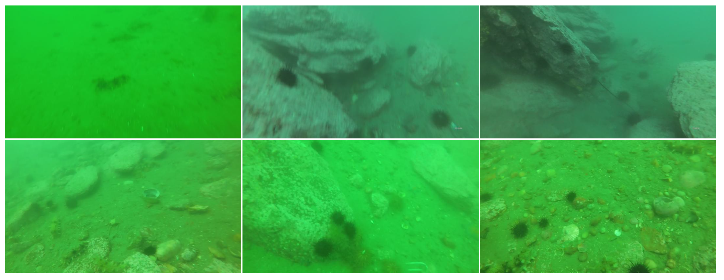
The URPC 2018 dataset is employed as our training and testing dataset. The URPC 2018 dataset contains underwater optical images acquired from the real-world shallow water environment. The images in the underwater environment exhibit severe degradation due to the backscatter and water absorption effect, as shown in Figure 6. Objects in underwater images usually have a very low SNR, especially small objects, which makes them more difficult to detect.

The URPC 2018 dataset contains four types of marine life objects, including holothurian, echinus, starfish, and scallop. The whole dataset is divided into the training set and testing set. The training set of the URPC 2018 contains 2901 labeled images, and the testing set contains 800 unlabeled images.

4.2. Evaluation Metric

We use the standard COCO [48] box evaluation metric as our performance criterion, and the mAP with different IOU thresholds is used as our main criterion. Specifically, in order to get the mAP, we need to calculate the AP for each category. The AP is given in Equation (5), and recall and precision in Equation (5) are calculated in Equation (6), n in Equation (5) is the total number of confidence thresholds, the $TP$, $FP$, and $FN$ in Equation (5) are the total number of true positive, false positive, and false positive samples, respectively. The mAP is average AP among all different classes, as listed in Equation (7). In Equation (7), $A{P}_k$ is the AP of k th class, and m is the total number of classes. In addition, we report the number of parameters as our additional criterion to evaluate the size of different models.

$$AP=\sum _{k=0}^{k=n-1}[Recall\left(k\right)-Recall(k+1)]\times Precision\left(k\right)$$

(5)

$$Precision=\frac{TP}{TP+FP},Recall=\frac{TP}{TP+FN}$$

(6)

$$mAP=\frac{1}{m}\sum _{k=1}^{k=m}A{P}_k$$

(7)

4.3. Implementation Details

We conduct our experiments on 1 NVIDIA RTX 3080 GPU with CUDA version 11.0 and PyTorch version 1.7.0. The operating system is Ubuntu 16.04 LTS. In all studies, the mini-batched stochastic gradient descent method is used to optimize the network. Our base learning rate is 0.1, and we set the momentum to 0.9 and the weight decay to 0.0001. For the backbone network, we have a smaller learning rate compared to the base learning rate, i.e., 0.5 times the base learning rate. The total learning epochs for all studies are set to 24. We decrease the learning rate at epoch 16 and epoch 22 by 0.1 times, respectively. Following the former studies [49], we refer to this setup as the 2× schedule. For better performance, we introduce the linear warming-up step at the beginning of training. The total warming-up step is specified as 2500 iterations, and the warming-up ratio is set to 0.00066667.

To reasonably compare the performance of different models and to evaluate models, we use the fixed-scale training approach, i.e., the image size is kept fixed, and all models in the comparison, unless otherwise specified, are assigned an input image size of $416\times 416$ during the training phase. During the inference phase, the input images for models participating in the comparison are likewise set to a size of $416\times 416$. The NMS is used as a post-processor for all models. It has an IOU threshold of 0.5 and a confidence threshold of 0.05.

We implement our experiment based on mmdetection codebase [49]. We follow [16] for the processing pipeline of training and test data.

4.4. Comparison with Other Models

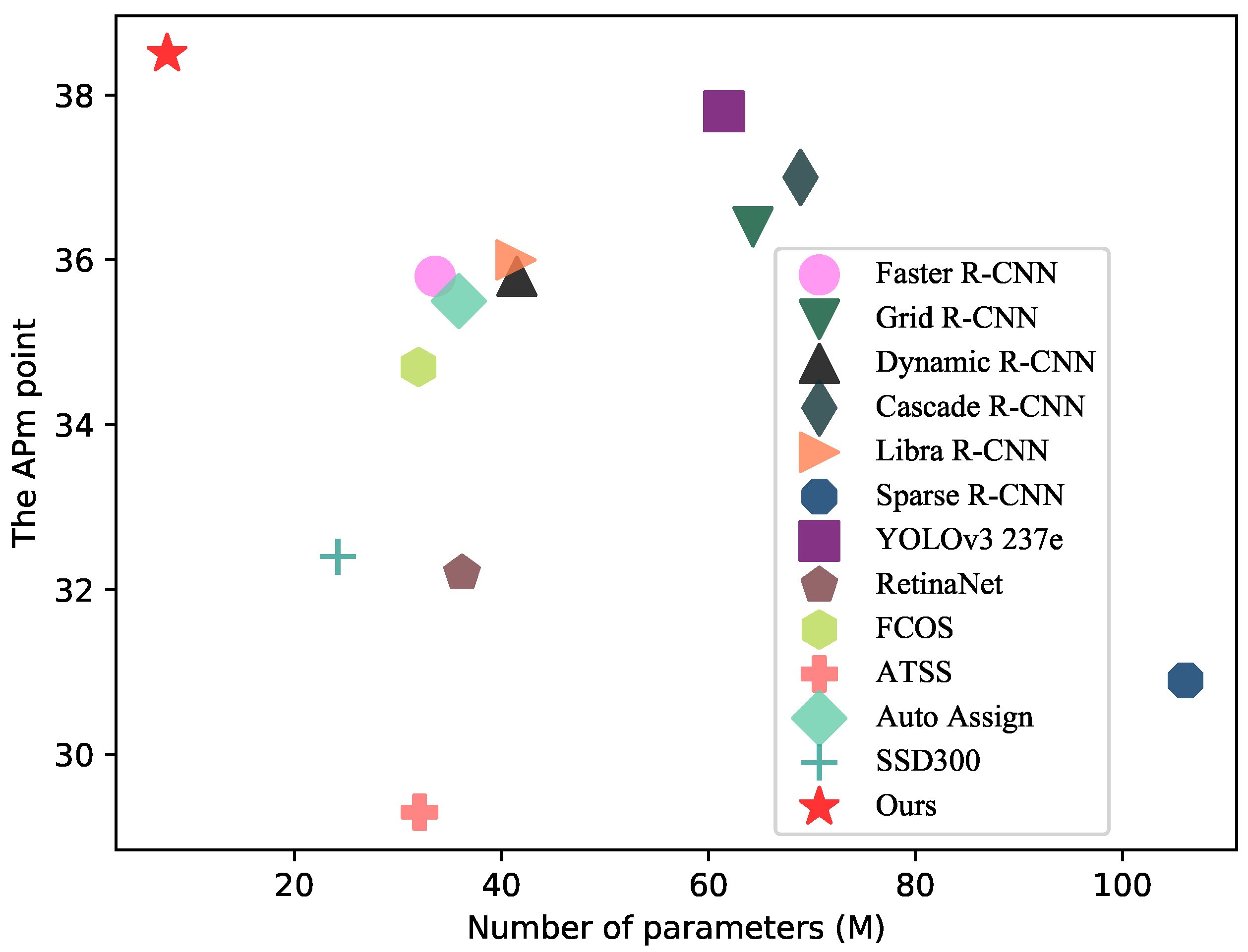
To validate the effectiveness of our model, we fully evaluate it on the URPC2018 dataset and compare it with the baseline model. RetinaNet [16], an advanced single-stage universal detector, shown impressive robustness and performance in general object detection, therefore we use it as our baseline model. We take into consideration both the number parameters and the performance, as shown in Figure 7.

Detailed comparisons are reported in Table 1. In Figure 7, the nearer the model is to the upper left corner of the coordinates, the better the overall performance of the model, i.e., having fewer parameters and better performance.

Our model is located in the top left corner of the Figure 7 and therefore has the fewest parameters and the best performance of all the models. As a result, our approach has the highest overall performance of all these models.

The proposed model achieves a 6.3 APm improvement over the baseline. Furthermore, our model gains 13.6 APm on small objects compared to the baseline model, indicating that our model is able to enhance the signal from feeble and small objects in the network. We also evaluate the performance of advanced two-stage detectors, such as faster R-CNN [13], grid R-CNN [50], dynamic R-CNN [51], cascade R-CNN [52], Libra R-CNN [53], and sparse R-CNN [54] on the URPC 2018 dataset. As can be seen from Table 1, we observe that these models exhibit a substantial performance degradation on smaller size underwater image data compared to larger size images in the air. Our model also substantially outperforms the aforementioned two-stage detectors both in terms of AP performance and parameter size.

In addition, we comprehensively evaluate the differences between our model and the latest one-stage detectors. Compared with 237 epoch trained YOLOv3 [21], our model outperforms it by 0.7 points, which also means our model converges faster than YOLOv3. For the classical lightweight detector SSD300 [15] and recent adaptive one-stage detector Auto Assign [20], our model outperforms them by 6.1 and 3.0 points, respectively. ATSS [19] is another adaptive one-stage detector that performs well in general object detection in air. Our model surpasses this model by 9.2 points in the small size underwater image condition. In addition, we evaluate the performance of the typical anchor-free one-stage detector FCOS [55] on small-sized underwater images, and we find that our detector outperforms this model by 3.8 points. It is noteworthy that our model has the fewest parameters of all the models noted above. We use the number of parameters as a measure of time-space complexity: the larger the number of parameters, the higher the time-space complexity. In addition, to test the real-time properties of the model, we conducted experiments on the RTX 3080; the model provided real-time detection at 22.6 fps.

Table 1. Comparison between models on URPC2018.

Method	#Param	AP	AP50	AP75	APs	APm	APl	Schedules
Two-Stage Method:
Faster R-CNN [13]	33.6 M	35.8	69.8	33.4	16.4	36.5	51.4	2×
Grid R-CNN [50]	64.3 M	36.4	69.9	34.1	15.3	37.4	51.2	2×
Dynamic R-CNN [51]	41.5 M	35.8	66.9	35.2	13.3	37.2	51.4	2×
Cascade R-CNN [52]	68.9 M	37.0	69.2	35.6	16.0	37.9	52.0	2×
Libra R-CNN [53]	41.4 M	36.0	68.8	33.7	16.4	36.7	51.2	2×
Sparse R-CNN [54]	106.1 M	30.9	61.2	27.8	16.2	30.8	46.2	2×
One-Stage Method:
YOLOv3 237e [21]	61.5 M	37.8	72.1	35.0	19.4	38.4	50.5	237e
RetinaNet [16]	36.2 M	32.2	65.3	28.2	9.2	32.6	48.0	2×
FCOS [55]	32.0 M	34.7	69.7	29.8	13.9	35.6	47.7	2×
ATSS [19]	32.1 M	29.3	62.1	22.9	13.5	30.9	36.0	2×
Auto Assign [20]	35.9 M	35.5	71.8	30.1	15.5	36.1	49.6	2×
SSD300 [15]	24.2 M	32.4	64.7	27.1	16.0	33.7	42.5	2×
Ours	7.7 M	38.5	76.3	32.7	22.8	39.3	49.0	2×

Table 1. Comparison between models on URPC2018.

Method	#Param	AP	AP50	AP75	APs	APm	APl	Schedules
Two-Stage Method:
Faster R-CNN [13]	33.6 M	35.8	69.8	33.4	16.4	36.5	51.4	2×
Grid R-CNN [50]	64.3 M	36.4	69.9	34.1	15.3	37.4	51.2	2×
Dynamic R-CNN [51]	41.5 M	35.8	66.9	35.2	13.3	37.2	51.4	2×
Cascade R-CNN [52]	68.9 M	37.0	69.2	35.6	16.0	37.9	52.0	2×
Libra R-CNN [53]	41.4 M	36.0	68.8	33.7	16.4	36.7	51.2	2×
Sparse R-CNN [54]	106.1 M	30.9	61.2	27.8	16.2	30.8	46.2	2×
One-Stage Method:
YOLOv3 237e [21]	61.5 M	37.8	72.1	35.0	19.4	38.4	50.5	237e
RetinaNet [16]	36.2 M	32.2	65.3	28.2	9.2	32.6	48.0	2×
FCOS [55]	32.0 M	34.7	69.7	29.8	13.9	35.6	47.7	2×
ATSS [19]	32.1 M	29.3	62.1	22.9	13.5	30.9	36.0	2×
Auto Assign [20]	35.9 M	35.5	71.8	30.1	15.5	36.1	49.6	2×
SSD300 [15]	24.2 M	32.4	64.7	27.1	16.0	33.7	42.5	2×
Ours	7.7 M	38.5	76.3	32.7	22.8	39.3	49.0	2×

4.5. Ablation Study and Analysis

In this paper, we provide further analysis to verify the effectiveness and superiority of each component of our model. We start with our baseline model, which obtains 32.2 APm points and 36.2 M parameters. After adding the lightweight hybrid transformer-based backbone, as we can see in

Table 2. Effectiveness of each part of our model.

Method	#Param	AP	AP50	AP75	APs	APm	APl
Baseline	36.2 M	32.2	65.3	28.2	9.2	32.6	48.0
Baseline + mobilevit	6.94 M	37.3	74.6	32.3	21.9	37.9	48.1
Baseline + mobilevit + FG-FPN	7.68 M	38.1	75.4	32.9	22.3	38.6	49.1
Baseline + mobilevit + FG-FPN + TTA	7.68 M	38.5	76.3	32.7	22.8	39.3	49.0

, the parameters of the model decreased by 29.26 M, whereas the APm performance increases by 5.1. It is clear that the lightweight backbone based on hybrid transformers gives the model an enormous boost and at the same time significantly reduces the number of parameters in the model. That gives us the insight that hybrid transformer-based networks, which extracts the global context information of the object quite well, can perform remarkably well on underwater optical images with relatively small sizes. We further add our fine-grained FPN (FG-FPN in Table 2) to the detector and find that it brings 0.8 points AP performance gains, and the number of parameters increases very slightly. It is also notable that our fine-grained FPN model can obtain a 0.4 AP point gain for the small object, which means the fine-grained FPN model is beneficial to small object detection. To further improve the performance of our model, test-time-augmentation (TTA) is introduced during the evaluation period and achieves an additional 0.4 AP point gain with no additional increase in the number of parameters.

4.6. URPC 2018 Error Analysis

To further analyze the detection results of our model, we show a detailed breakdown of results for the URPC 2018. We use the same methods and analysis tools as Redmon et al. [14]. All errors are classified into four types based on the following metrics:

• Localization (Loc):classification is correct, and $0.1<IOU<0.5$;
• Other (Oth):wrong classes, and $IOU>0.1$;
• Background (BG): $IOU<0.1$ for all objects;
• False Negative (FN): $IOU>0.5$, but the classification is wrong.

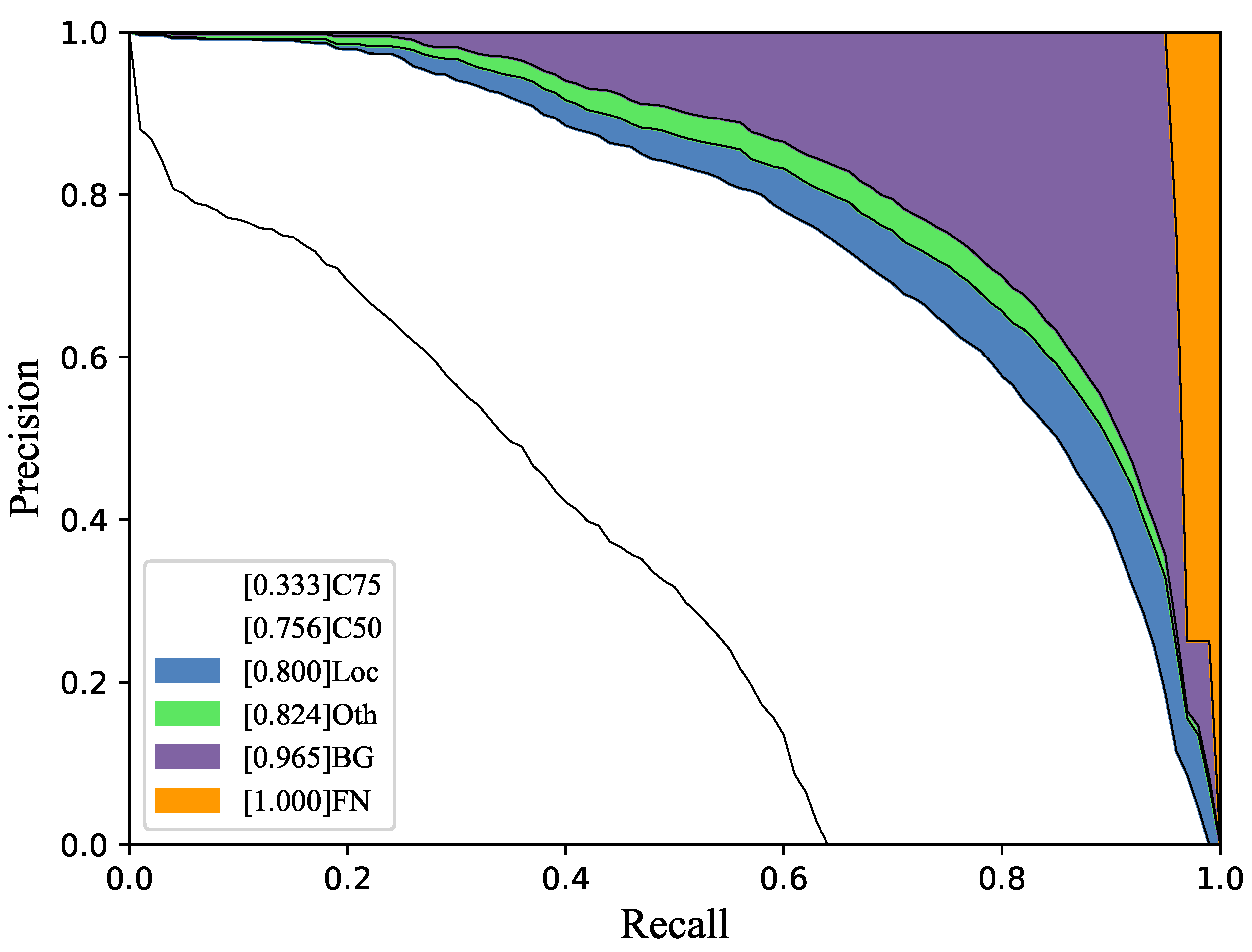
Figure 8 shows the breakdown error analysis for all four classes. In addition, Figure 8 gives a series of precision–recall curves at different conditions. As we can see, the main error contribution is still the BG error, which is mainly caused by objects with low SNR in underwater images. Our work used the fine-grained FPN to enhance the SNR of feeble and small objects, improving the small object APm performance from 21.9 to 22.3, which solved this problem to some extent.

4.7. Detection Results Analysis for Each Category

We analyze the precision–recall curves on each category of the URPC2018 dataset, as shown in Figure 9.

In general, there are four curves in Figure 9, corresponding to four categories in the dataset. All these curves are plotted with an IOU threshold of 0.5. The areas between the curves and the axes indicate the AP for the respective classes. It is illustrated in Figure 9 that our detector has the best detection performance for echinus. Among the four targets, the scallop has the worst detection. We empirically infer that the main reason for this is false positive samples caused by the presence of background noise (small rocks) on the seafloor. The echinus, on the other hand, is easier to be distinguished due to the large color difference.

4.8. Classification Analysis for Each Category

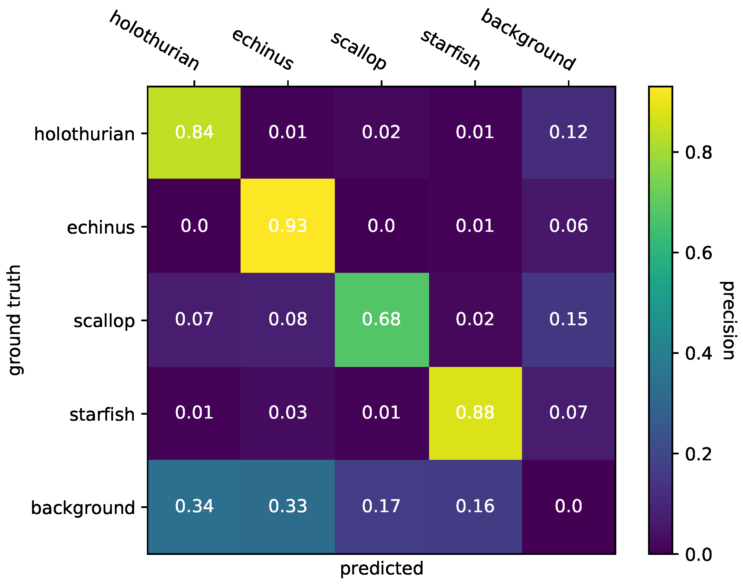
In order to further analyze the performance of the classifier on the URPC dataset, we dive deeply into the classification results of the classification branch and conduct the confusion matrix of the classification branch on the dataset, as presented in Figure 10.

In Figure 10, the values in the matrix are normalized, with the x-axis representing the ground truth and the y-axis representing the prediction. Generally speaking, our classification branch has relatively high accuracy on holothurian, echinus, and starfish, as all accuracy of those labels achieves 80%. However, there are still a few challenges in the classification branch. First, for starfish, scallops, echinus, and holothurian, the classification branch has a relatively worse performance on scallops, as scallops usually have a small size and are the same color as the background noise. Compared to scallops, the echinus has the best classification accuracy, as the echinus’s color is quite different from the background. Second, holothurian is the class most likely to be recognized as background of the four classes. This is because of the existence of long tail distribution in the URPC dataset, and holothurian is the class that has fewer numbers compared to all other classes, including background.

4.9. Analysis on Robustness of the Detector

The unmanned underwater vehicle continuously detects and senses while navigating [56,57,58], inevitably introducing different levels and types of motion blur noise to the underwater images. In addition, due to other disturbances such as Rayleigh scattering and Mie scattering, the images taken by the vehicle during motion will also have varying degrees of random noise disturbances [59,60]. To investigate the capability of our model to cope with the above noise disturbances, we make use of the methods used in the study of neural network robustness in atmospheric environments [61]. Gaussian noise, Poisson noise, and impulse noise are introduced to simulate the disturbances introduced by scattering and other factors, while motion blur, defocus blur, glass blur, and zoom blur are introduced to simulate the disturbances introduced by the motion of the vehicle. Based on this, we conduct a robustness analysis of our model on the small-size underwater optical image dataset.

Following [61], we define five different noise-severity levels, denoted as S, where a higher S indicates a more severe disturbance. We first evaluate the tendency of our model’s performance under seven different disturbances, as shown in Figure 11a. In the figure, the triangular symbols are the four types of blurred type noise, i.e., low-frequency noise, whereas the circles are the diffuse type of noise, i.e., high-frequency noise. It is clear from the figure that, for four types of blurred disturbances except for zoom noise, the model performance degradation is much slighter compared to high-frequency noise, which implies that our model is more sensitive to high-frequency disturbances, and, therefore, particles of impurities and plankton in the water column will have a larger impact on the model under very turbulent conditions. It is noted that the model is also highly sensitive to zoom noise, indicating that the detection performance of the model may receive a relatively large degree of impact when the vehicle is under high-speed operation, and, therefore, the optical perception and detection under high-speed operation is a potential issue to be further investigated. Furthermore, similar to the effect of zoom blur noise, we find that there is little difference between the three types of high frequency noise in terms of model performance. As for the remaining three types of blurred noise, the effects of the remaining three on the model are similar when the noise severity is relatively low; with an increase in severity, the glass blur noise exhibits the slightest effect on the model among the three, and the remaining two have similar outcomes.

In order to further analyze the robustness of our model and the baseline model in the presence of noise, we compare the performance of our model with that of the baseline model under different configurations, as shown in Figure 11b,f. It can be easily concluded that the interference of high-frequency noise in the model is much greater than that of low-frequency noise. Note that both for low-frequency noises, e.g., defocus blur, glass blur, and motion blur, and high-frequency noises, e.g., Gaussian noise, shot noise, and impulse noise, our model substantially surpasses the baseline model and is more robust.

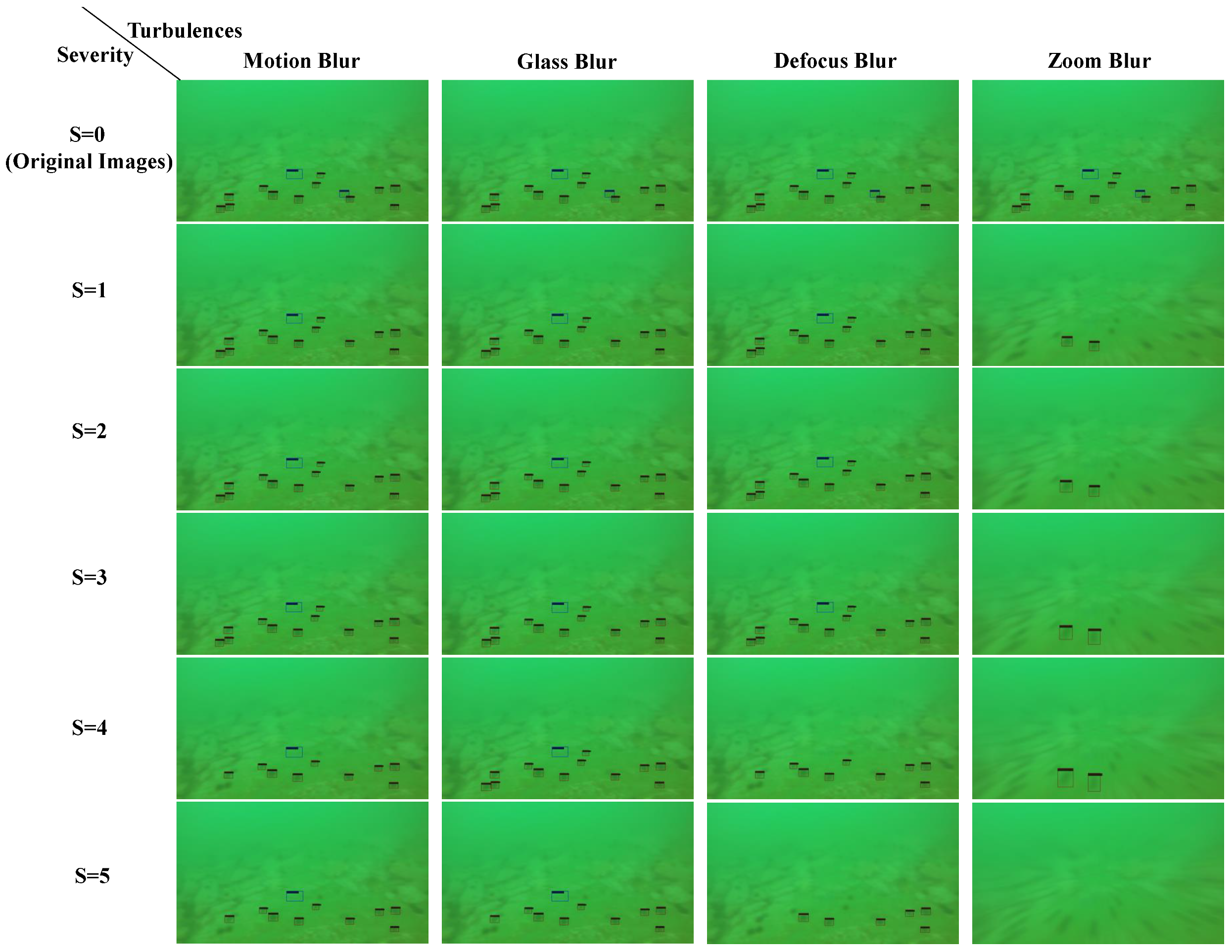
In order to better demonstrate the effects of different kinds of noise and different severity levels of noise on the model, we chose an image with multiple objects and a low object signal-to-noise ratio to visualize the detection effects of the model for high-frequency noise and low-frequency noise disturbances, respectively, as shown in Figure 12. From Figure 12, we can see that the objects are detected in the case where no noise is added; for the shot noise and the impulse noise, as S starts from 1, the objects are almost undetectable, whereas for Gaussian noise, when S is 1, only two targets can be detected, and with the increase of the S, the targets can also not be detected. For low-frequency noise, the circumstances are much better. From Figure 13, we can see that motion blur and glass blur have an effect only when S is 4 and 5, respectively, whereas Defocus blur has an effect when S is 4. Zoom blur, on the other hand, first emerged with a larger impact at S of 1, detecting only two targets, whereas when S is 5, no targets were detected.

4.10. Visualization of the Detection Results

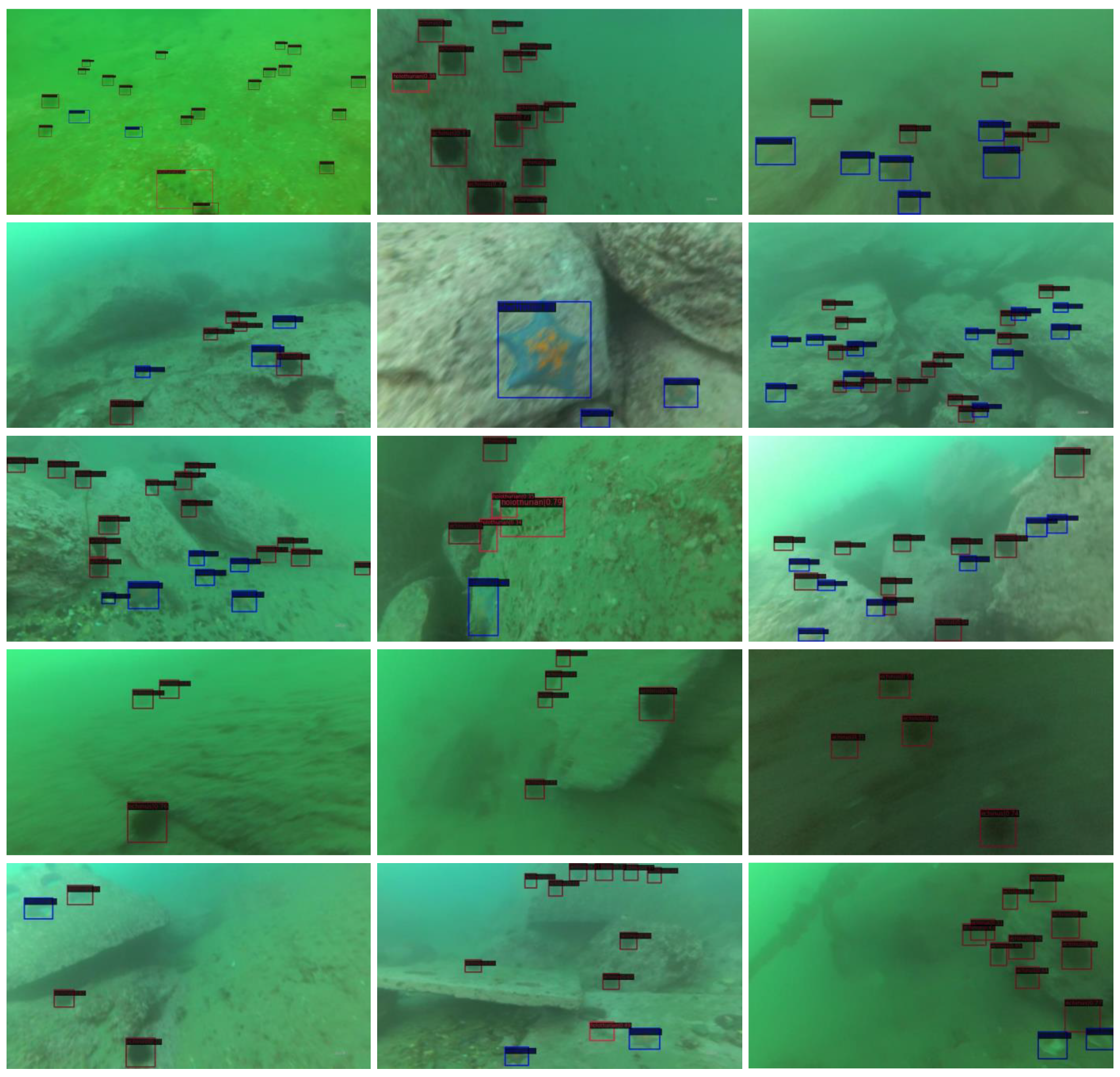
We test our model on the URPC2018 dataset. Figure 14 shows some detection results. It can be seen that objects in the images are small and clustered together, which makes them more difficult to detect. Our model can handle both small and large size objects. Moreover, for feeble objects in the image with a very low SNR, our model can still detect them.

5. Discussion

5.1. Lightweight Object Detection

Generally speaking, the computational capacity of autonomous underwater vehicles (AUV) is very restricted, and the current research on lightweight detectors in the field of underwater optical image object detection is still staying with the sparse design of the convolution kernel. With this solution, the number of model parameters can be effectively reduced without a significant decrease in the detection accuracy of the model. However, the question is whether this method changes the local relationship modeling, and whether the model does not gain significantly from reducing the number of parameters in the actual inference process. In this paper, we use a transformer-CNN hybrid network to capture global relations and solve the slow inference problem caused by the transformer network. Extensive experiments have demonstrated that the method in this paper can obtain better sensing capability of feeble objects, and the number of parameters of the model is much lower than that of the baseline model. However, in the hybrid network, the space–time complexity of the transformer layer is still the square of the input scale. Future research will focus on solving the quadratic space–time complexity of the transformer layer in the hybrid network in order to reduce the computational scale further.

5.2. Underwater Feeble and Small Object Detection

In underwater optical images, the problem of feeble and small object detection is a difficult and important problem. Previous efforts have used FPNs and short-connected FPNs to enhance the model’s sensing ability for feeble objects, but there is still the problem of low-level feeble objects’ signals being gradually fused and overwhelmed. In this paper, the proposed FG-FPN uses cumulative bridging to effectively strengthen the signal, which can effectively improve the detection ability of the model for feeble objects. However, the input feeble object signal still has the problem of low SNR. How to remove the noises and thus improve the SNR of the feeble and small objects’ signals will be a very valuable direction for future theoretical and engineering research.

6. Conclusions

In this paper, we present a transformer-based hybrid network for real-time underwater feeble and small object detection. To tackle the signal vanishing problem for feeble and small objects in the deep neural network, a fine-grained FPN module is designed to cumulatively fuse low-level and high-level features. A lightweight transformer-based hybrid backbone is introduced to exploit the global context information, allowing feeble and small objects to be detected efficiently and effectively. Moreover, the memory cost-free method is introduced to improve the performance of our detector without additional parameters. Due to the energy and weight restrictions, there is extremely limited computing resources that could be carried by underwater vehicles; thus, it is significant to pursue fewer parameters for applications in the underwater environment. Although our model has achieved relatively small results in terms of the number of parameters, there is still room for further improvement in terms of the actual speed of the device.

In the future, we will focus on distilling the knowledge from our trained detector to a smaller detector with comparable performance. In addition, object detection and sensing in an open underwater environment is very meaningful. The study of object detection in complex open underwater environments helps to apply the algorithms to realistic scenarios. We will further investigate object detection in open underwater environments based on lightweight detectors.

References

1. Moniruzzaman, M.; Islam, S.M.S.; Bennamoun, M.; Lavery, P. Deep learning on underwater marine object detection: A survey. In Proceedings of the Advanced Concepts for Intelligent Vision Systems: 18th International Conference, ACIVS 2017, Antwerp, Belgium, 18–21 September 2017; Springer: Berlin/Heidelberg, Germany, 2017; pp. 150–160. [Google Scholar]
2. Fayaz, S.; Parah, S.A.; Qureshi, G. Underwater object detection: Architectures and algorithms–a comprehensive review. Multimed. Tools Appl. 2022, 81, 20871–20916. [Google Scholar] [CrossRef]
3. Er, M.J.; Jie, C.; Zhang, Y.; Gao, W. Research Challenges, Recent Advances and Benchmark Datasets in Deep-Learning-Based Underwater Marine Object Detection: A Review. TechRxiv 2022. [Google Scholar] [CrossRef]
4. Moniruzzaman, M.; Islam, S.M.S.; Lavery, P.; Bennamoun, M. Faster R-CNN based deep learning for seagrass detection from underwater digital images. In Proceedings of the 2019 Digital Image Computing: Techniques and Applications (DICTA), Perth, Australia, 2–4 December 2019; pp. 1–7. [Google Scholar]
5. Tian, M.; Li, X.; Kong, S.; Wu, L.; Yu, J. A modified YOLOv4 detection method for a vision-based underwater garbage cleaning robot. Front. Inf. Technol. Electron. Eng. 2022, 23, 1217–1228. [Google Scholar] [CrossRef]
6. Wang, Y.; Tang, C.; Cai, M.; Yin, J.; Wang, S.; Cheng, L.; Wang, R.; Tan, M. Real-time underwater onboard vision sensing system for robotic gripping. IEEE Trans. Instrum. Meas. 2020, 70, 5002611. [Google Scholar] [CrossRef]
7. Zhang, W.; Dong, L.; Zhang, T.; Xu, W. Enhancing underwater image via color correction and bi-interval contrast enhancement. Signal Process. Image Commun. 2021, 90, 116030. [Google Scholar] [CrossRef]
8. Han, M.; Lyu, Z.; Qiu, T.; Xu, M. A review on intelligence dehazing and color restoration for underwater images. IEEE Trans. Syst. Man Cybern. Syst. 2018, 50, 1820–1832. [Google Scholar] [CrossRef]
9. Wang, N.; Zheng, B.; Zheng, H.; Yu, Z. Feeble object detection of underwater images through LSR with delay loop. Opt. Express 2017, 25, 22490–22498. [Google Scholar] [CrossRef]
10. Song, Y.; He, B.; Liu, P. Real-time object detection for AUVs using self-cascaded convolutional neural networks. IEEE J. Ocean. Eng. 2019, 46, 56–67. [Google Scholar] [CrossRef]
11. Zhang, M.; Xu, S.; Song, W.; He, Q.; Wei, Q. Lightweight underwater object detection based on yolo v4 and multi-scale attentional feature fusion. Remote Sens. 2021, 13, 4706. [Google Scholar] [CrossRef]
12. Shorten, C.; Khoshgoftaar, T.M. A survey on image data augmentation for deep learning. J. Big Data 2019, 6, 60. [Google Scholar] [CrossRef]
13. Ren, S.; He, K.; Girshick, R.; Sun, J. Faster r-cnn: Towards real-time object detection with region proposal networks. In Proceedings of the 29th Annual Conference on Neural Information Processing Systems 2015, Montreal, QC, Canada, 7–12 December 2015; Volume 28. [Google Scholar]
14. Redmon, J.; Divvala, S.; Girshick, R.; Farhadi, A. You only look once: Unified, real-time object detection. In Proceedings of the IEEE Conference on Computer Vision and Pattern Recognition, Las Vegas, NV, USA, 26 June–1 July 2016; pp. 779–788. [Google Scholar]
15. Liu, W.; Anguelov, D.; Erhan, D.; Szegedy, C.; Reed, S.; Fu, C.Y.; Berg, A.C. Ssd: Single shot multibox detector. In Proceedings of the Computer Vision–ECCV 2016: 14th European Conference, Amsterdam, The Netherlands, 11–14 October 2016; Springer: Berlin/Heidelberg, Germany, 2016; pp. 21–37. [Google Scholar]
16. Lin, T.Y.; Goyal, P.; Girshick, R.; He, K.; Dollár, P. Focal loss for dense object detection. In Proceedings of the IEEE International Conference on Computer Vision, Venice, Italy, 22–29 October 2017; pp. 2980–2988. [Google Scholar]
17. Carion, N.; Massa, F.; Synnaeve, G.; Usunier, N.; Kirillov, A.; Zagoruyko, S. End-to-end object detection with transformers. In Proceedings of the Computer Vision–ECCV 2020: 16th European Conference, Glasgow, UK, 23–28 August 2020; Springer: Berlin/Heidelberg, Germany, 2020; pp. 213–229. [Google Scholar]
18. Zhu, X.; Su, W.; Lu, L.; Li, B.; Wang, X.; Dai, J. Deformable detr: Deformable transformers for end-to-end object detection. arXiv 2020, arXiv:2010.04159. [Google Scholar]
19. Zhang, S.; Chi, C.; Yao, Y.; Lei, Z.; Li, S.Z. Bridging the gap between anchor-based and anchor-free detection via adaptive training sample selection. In Proceedings of the IEEE/CVF Conference on Computer Vision and Pattern Recognition, Seattle, WA, USA, 13–19 June 2020; pp. 9759–9768. [Google Scholar]
20. Zhu, B.; Wang, J.; Jiang, Z.; Zong, F.; Liu, S.; Li, Z.; Sun, J. Autoassign: Differentiable label assignment for dense object detection. arXiv 2020, arXiv:2007.03496. [Google Scholar]
21. Redmon, J.; Farhadi, A. Yolov3: An incremental improvement. arXiv 2018, arXiv:1804.02767. [Google Scholar]
22. Bochkovskiy, A.; Wang, C.Y.; Liao, H.Y.M. Yolov4: Optimal speed and accuracy of object detection. arXiv 2020, arXiv:2004.10934. [Google Scholar]
23. Peng, F.; Miao, Z.; Li, F.; Li, Z. S-FPN: A shortcut feature pyramid network for sea cucumber detection in underwater images. Expert Syst. Appl. 2021, 182, 115306. [Google Scholar] [CrossRef]
24. Zong, C.; Wang, H.; Wan, Z. An improved 3D point cloud instance segmentation method for overhead catenary height detection. Comput. Electr. Eng. 2022, 98, 107685. [Google Scholar] [CrossRef]
25. Yang, M.; Wang, H.; Hu, K.; Yin, G.; Wei, Z. IA-Net: An Inception–Attention-Module-Based Network for Classifying Underwater Images From Others. IEEE J. Ocean. Eng. 2022, 47, 704–717. [Google Scholar] [CrossRef]
26. Liao, L.; Du, L.; Guo, Y. Semi-supervised SAR target detection based on an improved faster R-CNN. Remote Sens. 2021, 14, 143. [Google Scholar] [CrossRef]
27. Zhou, G.; Li, W.; Zhou, X.; Tan, Y.; Lin, G.; Li, X.; Deng, R. An innovative echo detection system with STM32 gated and PMT adjustable gain for airborne LiDAR. Int. J. Remote Sens. 2021, 42, 9187–9211. [Google Scholar] [CrossRef]
28. Zhou, G.; Zhou, X.; Song, Y.; Xie, D.; Wang, L.; Yan, G.; Hu, M.; Liu, B.; Shang, W.; Gong, C.; et al. Design of supercontinuum laser hyperspectral light detection and ranging (LiDAR)(SCLaHS LiDAR). Int. J. Remote Sens. 2021, 42, 3731–3755. [Google Scholar] [CrossRef]
29. Wu, X.; Hong, D.; Tian, J.; Chanussot, J.; Li, W.; Tao, R. ORSIm detector: A novel object detection framework in optical remote sensing imagery using spatial-frequency channel features. IEEE Trans. Geosci. Remote Sens. 2019, 57, 5146–5158. [Google Scholar] [CrossRef] [Green Version]
30. Wu, X.; Hong, D.; Chanussot, J. UIU-Net: U-Net in U-Net for infrared small object detection. IEEE Trans. Image Process. 2022, 32, 364–376. [Google Scholar] [CrossRef]
31. Zhou, G.; Li, C.; Zhang, D.; Liu, D.; Zhou, X.; Zhan, J. Overview of underwater transmission characteristics of oceanic LiDAR. IEEE J. Sel. Top. Appl. Earth Obs. Remote Sens. 2021, 14, 8144–8159. [Google Scholar] [CrossRef]
32. Liu, L.; Zhang, S.; Zhang, L.; Pan, G.; Yu, J. Multi-UUV Maneuvering Counter-Game for Dynamic Target Scenario Based on Fractional-Order Recurrent Neural Network. IEEE Trans. Cybern. 2022, 1–14. [Google Scholar] [CrossRef]
33. Xie, B.; Li, S.; Lv, F.; Liu, C.H.; Wang, G.; Wu, D. A collaborative alignment framework of transferable knowledge extraction for unsupervised domain adaptation. IEEE Trans. Knowl. Data Eng. 2022; Early Access. [Google Scholar] [CrossRef]
34. Zhao, Z.; Liu, Y.; Sun, X.; Liu, J.; Yang, X.; Zhou, C. Composited FishNet: Fish Detection and Species Recognition From Low-Quality Underwater Videos. IEEE Trans. Image Process. 2021, 30, 4719–4734. [Google Scholar] [CrossRef] [PubMed]
35. Sandler, M.; Howard, A.; Zhu, M.; Zhmoginov, A.; Chen, L.C. Mobilenetv2: Inverted residuals and linear bottlenecks. In Proceedings of the IEEE Conference on Computer Vision and Pattern Recognition, Salt Lake City, UT, USA, 18–23 June 2018; pp. 4510–4520. [Google Scholar]
36. Chollet, F. Xception: Deep learning with depthwise separable convolutions. In Proceedings of the IEEE Conference on Computer Vision and Pattern Recognition, Honolulu, HI, USA, 21–26 July 2017; pp. 1251–1258. [Google Scholar]
37. Lin, T.Y.; Dollár, P.; Girshick, R.; He, K.; Hariharan, B.; Belongie, S. Feature pyramid networks for object detection. In Proceedings of the IEEE Conference on Computer Vision and Pattern Recognition, Honolulu, HI, USA, 21–26 July 2017; pp. 2117–2125. [Google Scholar]
38. Yeh, C.H.; Lin, C.H.; Kang, L.W.; Huang, C.H.; Lin, M.H.; Chang, C.Y.; Wang, C.C. Lightweight deep neural network for joint learning of underwater object detection and color conversion. IEEE Trans. Neural Netw. Learn. Syst. 2021, 33, 6129–6143. [Google Scholar] [CrossRef]
39. Tan, C.; DanDan, C.; Huang, H.; Yang, Q.; Huang, X. A Lightweight Underwater Object Detection Model: FL-YOLOV3-TINY. In Proceedings of the 2021 IEEE 12th Annual Information Technology, Electronics and Mobile Communication Conference (IEMCON), Vancouver, BC, Canada, 27–30 October 2021; pp. 0127–0133. [Google Scholar]
40. Mehta, S.; Rastegari, M. Mobilevit: Light-weight, general-purpose, and mobile-friendly vision transformer. arXiv 2021, arXiv:2110.02178. [Google Scholar]
41. Dosovitskiy, A.; Beyer, L.; Kolesnikov, A.; Weissenborn, D.; Zhai, X.; Unterthiner, T.; Dehghani, M.; Minderer, M.; Heigold, G.; Gelly, S.; et al. An image is worth 16x16 words: Transformers for image recognition at scale. arXiv 2020, arXiv:2010.11929. [Google Scholar]
42. Tong, K.; Wu, Y.; Zhou, F. Recent advances in small object detection based on deep learning: A review. Image Vis. Comput. 2020, 97, 103910. [Google Scholar] [CrossRef]
43. Liu, Y.; Sun, P.; Wergeles, N.; Shang, Y. A survey and performance evaluation of deep learning methods for small object detection. Expert Syst. Appl. 2021, 172, 114602. [Google Scholar] [CrossRef]
44. Sun, W.; Dai, L.; Zhang, X.; Chang, P.; He, X. RSOD: Real-time small object detection algorithm in UAV-based traffic monitoring. Appl. Intell. 2022, 52, 8448–8463. [Google Scholar] [CrossRef]
45. Qi, G.; Zhang, Y.; Wang, K.; Mazur, N.; Liu, Y.; Malaviya, D. Small Object Detection Method Based on Adaptive Spatial Parallel Convolution and Fast Multi-Scale Fusion. Remote Sens. 2022, 14, 420. [Google Scholar] [CrossRef]
46. Chen, Q.; Wang, Y.; Yang, T.; Zhang, X.; Cheng, J.; Sun, J. You only look one-level feature. In Proceedings of the IEEE/CVF Conference on Computer Vision and Pattern Recognition, Nashville, TN, USA, 19–25 June 2021; pp. 13039–13048. [Google Scholar]
47. Lin, W.H.; Zhong, J.X.; Liu, S.; Li, T.; Li, G. RoIMix: Proposal-fusion among multiple images for underwater object detection. In Proceedings of the ICASSP 2020—2020 IEEE International Conference on Acoustics, Speech and Signal Processing (ICASSP), Barcelona, Spain, 4–8 May 2020; pp. 2588–2592. [Google Scholar]
48. Lin, T.Y.; Maire, M.; Belongie, S.; Hays, J.; Perona, P.; Ramanan, D.; Dollár, P.; Zitnick, C.L. Microsoft coco: Common objects in context. In Proceedings of the European Conference on Computer Vision, Zurich, Switzerland, 6–12 September 2014; Springer: Berlin/Heidelberg, Germany, 2014; pp. 740–755. [Google Scholar]
49. Chen, K.; Wang, J.; Pang, J.; Cao, Y.; Xiong, Y.; Li, X.; Sun, S.; Feng, W.; Liu, Z.; Xu, J.; et al. MMDetection: Open mmlab detection toolbox and benchmark. arXiv 2019, arXiv:1906.07155. [Google Scholar]
50. Lu, X.; Li, B.; Yue, Y.; Li, Q.; Yan, J. Grid r-cnn. In Proceedings of the IEEE/CVF Conference on Computer Vision and Pattern Recognition, Long Beach, CA, USA, 15–20 June 2019; pp. 7363–7372. [Google Scholar]
51. Zhang, H.; Chang, H.; Ma, B.; Wang, N.; Chen, X. Dynamic R-CNN: Towards high quality object detection via dynamic training. In Proceedings of the Computer Vision–ECCV 2020: 16th European Conference, Glasgow, UK, 23–28 August 2020; Springer: Berlin/Heidelberg, Germany, 2020; pp. 260–275. [Google Scholar]
52. Cai, Z.; Vasconcelos, N. Cascade R-CNN: High quality object detection and instance segmentation. IEEE Trans. Pattern Anal. Mach. Intell. 2019, 43, 1483–1498. [Google Scholar] [CrossRef] [PubMed] [Green Version]
53. Pang, J.; Chen, K.; Shi, J.; Feng, H.; Ouyang, W.; Lin, D. Libra r-cnn: Towards balanced learning for object detection. In Proceedings of the IEEE/CVF Conference on Computer Vision and Pattern Recognition, Long Beach, CA, USA, 15–20 June 2019; pp. 821–830. [Google Scholar]
54. Sun, P.; Zhang, R.; Jiang, Y.; Kong, T.; Xu, C.; Zhan, W.; Tomizuka, M.; Li, L.; Yuan, Z.; Wang, C.; et al. Sparse r-cnn: End-to-end object detection with learnable proposals. In Proceedings of the IEEE/CVF Conference on Computer Vision and Pattern Recognition, Nashville, TN, USA, 19–25 June 2021; pp. 14454–14463. [Google Scholar]
55. Tian, Z.; Shen, C.; Chen, H.; He, T. Fcos: Fully convolutional one-stage object detection. In Proceedings of the IEEE/CVF International Conference on Computer Vision, Seoul, Republic of Korea, 27 October–2 November 2019; pp. 9627–9636. [Google Scholar]
56. Jin, H.S.; Cho, H.; Jiafeng, H.; Lee, J.H.; Kim, M.J.; Jeong, S.K.; Ji, D.H.; Joo, K.; Jung, D.; Choi, H.S. Hovering control of UUV through underwater object detection based on deep learning. Ocean. Eng. 2022, 253, 111321. [Google Scholar] [CrossRef]
57. Álvarez-Tuñón, O.; Jardón, A.; Balaguer, C. Generation and processing of simulated underwater images for infrastructure visual inspection with UUVs. Sensors 2019, 19, 5497. [Google Scholar] [CrossRef] [Green Version]
58. Watson, S.; Duecker, D.A.; Groves, K. Localisation of unmanned underwater vehicles (UUVs) in complex and confined environments: A review. Sensors 2020, 20, 6203. [Google Scholar] [CrossRef]
59. Yang, M.; Hu, J.; Li, C.; Rohde, G.; Du, Y.; Hu, K. An in-depth survey of underwater image enhancement and restoration. IEEE Access 2019, 7, 123638–123657. [Google Scholar] [CrossRef]
60. Anwar, S.; Li, C. Diving deeper into underwater image enhancement: A survey. Signal Process. Image Commun. 2020, 89, 115978. [Google Scholar] [CrossRef]
61. Hendrycks, D.; Dietterich, T.G. Benchmarking neural network robustness to common corruptions and surface variations. arXiv 2018, arXiv:1807.01697. [Google Scholar]
Figure 1. Feeble and small objects in the underwater image. The image appears severely degraded, showing low contrast, non-uniform illumination, and blurring: (a) shows the detection results, (b) shows the feeble and small object that is hard to detect, where the object’s SNR is −3.7 dB, and (c) shows the object with SNR equal to −2.7 dB.
Remotesensing 15 01076 g001
Figure 2. Overview schematic diagram of our algorithm. The images are fed into the network, first through a series of enhancements, then through a hybrid backbone network to extract features and a fine-grained pyramid to enhance the features. Finally, TTA is used to improve recognition accuracy.
Remotesensing 15 01076 g002
Figure 3. Overview of our detector. The input of the network is a color image with three channels, and the lightweight backbone is applied to extract multiscale features from the input image. A novel fine-grained FPN is applied to get feeble and small object friendly features. The hyperparameter L in the backbone is the repeated times of transformer blocks for each MobileVit module. The s in the MBV2 module is the down-sampling stride number relative to each module’s input.
Remotesensing 15 01076 g003
Figure 4. Mobilevit block. Compared to pure CNN or pure transformer, the Mobilevit block comprises the benefits of CNN and transformer together, and thus can get meaningful global context features.
Remotesensing 15 01076 g004
Figure 5. Fine-grained FPN. Compared to a standard FPN module, The fine-grained FPN directly builds the connection from the low-level feature to high-level features and avoids the context information being lost.
Remotesensing 15 01076 g005
Figure 6. Degraded underwater images in URPC2018. Images taken underwater usually present severe degradation because of the light window effect and the light scatter effect.
Remotesensing 15 01076 g006
Figure 7. Trade-offs between performance and number of parameters for each model. The x-axis is the number of parameters of the model and the y-axis is the APm point of the model. The closer the model is to the upper left corner, the better the model performs. Our model is represented by a pentagram. Considering both the number of parameters and performance, our model has the best performance among many models.
Remotesensing 15 01076 g007
Figure 8. Error analysis on URPC 2018. We decompose the error of our detector on the URPC2018 dataset and determine that the main error contribution is the BG error, which means the detector has difficulty finding the object in a severely degraded image. To this end, our work introduced a novel fine-grained FPN module and enhanced the feature representation of feeble and small objects.
Remotesensing 15 01076 g008
Figure 9. Precision–recall curves for each category in URPC 2018. There are four categories in the dataset. The area under the curve indicates the performance of that model in the specific category. The larger the area, the better the model performance.
Remotesensing 15 01076 g009
Figure 10. Confusion matrix for the classification branch. All values in the matrix are normalized, and color depths in the matrix represent the magnitude of the different values. As we do not detect the background, the diagonal value of the background is zero.
Remotesensing 15 01076 g010
Figure 11. Robustness analysis of our model under different noise disturbances. In (a), the triangle symbol indicates low-frequency noise, and the circle icon indicates high-frequency noise. The red bars in (bf) are our model performance, whereas the blue bars are the baseline. From (b) to (f), the severity of the noise is sequentially increased. (a) The performance trend of our model under different levels of noise disturbance. (b) Comparison of model performances under different noise disturbances for a noise severity of 1. (c) Comparison of model performances under different noise disturbances for a noise severity of 2. (d) Comparison of model performances under different noise disturbances for a noise severity of 3. (e) Comparison of model performances under different noise disturbances for a noise severity of 4. (f) Comparison of model performances under different noise disturbances for a noise severity of 5.
Remotesensing 15 01076 g011
Figure 12. Visualization of the detection results of our model in the scenarios with three types of noise and five varying severity levels of input noise disturbances. In the figure, S is the severity of the noise, each column is the detection result under the same noise, and each row is the detection result of the model under different noise disturbances of the same severity. It is noticeable that S = 0 is the model detection result without additional noise.
Remotesensing 15 01076 g012
Figure 13. Visualization of the model’s image detection results for different levels of noise severity in the scenario of four types of blurred noise that may be caused by movement. In the figure, S represents the same meaning as in Figure 12. In contrast to the previous figure, we use four different kinds of blurred noise here.
Remotesensing 15 01076 g013
Figure 14. Detection results of our proposed model on the URPC 2018 dataset. The blue boxes are starfish and the red boxes are echinus. Almost all objects are located with a bounding box, although for some objects, it is hard to pick it out. Our detector achieved relatively good qualitative results.
Remotesensing 15 01076 g014