Article

How Can Ecological Land Be Deployed to Cool the Surface Thermal Environment? A Case Study from the Perspectives of Patch and Network

1
College of Geoscience and Surveying Engineering, China University of Mining and Technology-Beijing, Beijing 100083, China
2
Ningxia Data and Application Center of High Resolution Earth Observation System, Ningxia Institute of Remote Sensing Survey, Yinchuan 750021, China
3
Satellite Application Center for Ecology and Environment, Ministry of Ecology and Environment, Beijing 100094, China
*
Author to whom correspondence should be addressed.
Remote Sens. 2023, 15(4), 1061; https://doi.org/10.3390/rs15041061
Submission received: 23 December 2022 / Revised: 6 February 2023 / Accepted: 7 February 2023 / Published: 15 February 2023
(This article belongs to the Section Environmental Remote Sensing)

Abstract

:
Changes in climate and rapid urbanization have aggravated the urban heat island effect, and a reasonable means to reduce temperature increases in the surface thermal environment is urgently needed. We integrated the research perspectives of patch and network, taking Yinchuan metropolitan region as the research area, and reduced the surface thermal environment through the rational allocation of ecological land. For patch, a correlation analysis and linear regression were used to study the impact of landscape composition and spatial configuration on the surface thermal environment. For network, the thermal source patches were determined based on the morphological spatial pattern analysis (MSPA) method, the thermal resistance surface was calculated based on the minimum cumulative resistance model, and the pinch points and corridors that prevented the surface thermal environment from circulating were determined based on circuit theory. Finally, ecological land with a cooling effect was deployed at the pinch point to prevent heat patch from spreading and thus connect to larger heat networks, and the regional cooling effect was estimated. The results were as follows: (1) The fitting precision of landscape factors and the surface temperature was in the order of area ratio of ecological land > shape index > fragmentation index. When the area ratio of ecological land was greater than 61%, the patch shape was simple, the degree of fragmentation was low, and the cooling effect was the most obvious. (2) Then, 34 corridors, 44 pinch points, and 54 grids of ecological land were identified for deployment. (3) After the deployment of ecological land, the simulated cooling effect was between 0.04 and 6.02 °C, with an average decline of 2.16 °C. This research case offers approaches for mitigating temperature increases in the surface thermal environment and improving the sustainable development of cities (regions), and it serves as a reference for improving the ecological environmental quality in arid and semiarid areas.

1. Introduction

The urban heat island (UHI) effect is causing increasing harm to humans and the natural environment due to global warming. Surface thermal environment cooling of the city is a very concerning issue [1,2]. Numerous studies have shown that increasing vegetation, water, wetland, and other types of ecological land can mitigate increases in the surface temperature [3,4,5]. The most important step in ecological land deployment is to determine the deployment position. Simultaneously, it is necessary to consider the comprehensive influence of other factors [5,6,7]. For example, to maximize the cooling effect, when deploying ecological land, one should consider the amount of area needed, whether the shape should be simple or complex, and whether the patches should be compact or loose [8].
Many researchers have studied landscape patterns [9] based on patch mosaics at the patch level (size, shape, composition, and type) [10] to analyze the impact of ecological land types on the intensity of heat island mitigation [11]. The cooling effect on the surface thermal environment is significantly influenced by a reasonable area ratio of the ecological land area and spatial layout. Based on the patch perspective, landscape composition and landscape configuration [12,13] affect the cooling effect of ecological land [14]. Commonly used study units include land-use classifications, grids, and neighborhoods. The factors that influence the mitigation of UHIs include the area ratio and the complexity of urban green space (UGS) [15]; the cooling effect of large UGS patches is more obvious, and there is a threshold between the patch area and the cooling effect [16,17]. The area ratio of water or green space in a landscape is positively correlated with its cooling effect [18].
Based on the network perspective, by calculating the connectivity of thermal patches in the landscape pattern, modeling and evaluation are performed to provide a reference for cooling the surface thermal environment [19,20,21]. UHI patches can be regarded as heat patches, and their intensity increases with the connectivity between patches [5,22]. Circuit theory analyzes surface thermal environmental connectivity by computing least-cost paths between landscape nodes [23,24,25], representing the degree of connectivity between nodes with a resistance raster map [5]. The connectivity between urban parks and green corridors was calculated using graph theory and Conefor software, and recommendations were provided for the development of ecological, green infrastructure networks [20] to improve the surface thermal environment. Zhaowu Yu [25] proposed a conceptual framework for assessing and mitigating the UHI graphically in 2021, but no mitigation measures or simulated cooling effects were proposed. Utilizing the MSPA approach to describe UHI patterns and networks [26,27] can facilitate a determination of the spatial distribution of UHIs on a regional scale and the development of effective mitigation strategies [28]. Zhaowu Yu [24] built a UHI network using MSPA and circuit theory, identifying pinch points and corridors of heat circulation and adding ecological land at pinch points to block heat spread and reduce heat island intensity. Based on a network analysis, Zahra Mokhtari [29] calculated the connectivity of the heat sink or heat source points using the connectivity cost between resistive surfaces or patches. In terms of the network, it provides urban planners with an optimization scheme of UGS spatial patterns to mitigate urban temperature increases.
To summarize, the pieces of research on cooling the surface thermal environment from the patch perspective and the network perspective have their own focus and limitations. Research from the network perspective can determine the location of the ecological land to be deployed but it cannot recommend the parameters, such as area, shape, and fragmentation, of the ecological land to be deployed [29]. Research from the patch perspective can derive the cooling effects of landscape composition and landscape configuration on ecological land classes; however, it is hard to describe the overview of the surface thermal environment and the connectivity between patches [30], and it is difficult to precisely locate the spatial pattern and network [25] of the surface thermal environment to propose effective strategies to cool the LST [31]. This case integrates the two perspectives of patch and network for cooling the surface thermal environment and answers the following three key questions: (1) Which factor has the greatest impact on the allocation of ecological land, concerning area, shape, and fragmentation? (2) Where are the cooling points located (corridors and pinch points where thermal patches spread)? (3) How does the cooling effect work? This case can provide a coherent analytical process for research on cooling the surface thermal environment, from locating pinch points to allocating suitable ecological land, and blocking the connection between heat spots, which can effectively prevent the formation of a larger heat network due to the connection of heat spots. This case can also provide references for cooling the surface thermal environment and improving urban (regional) sustainable development.

2. Study Area and Data

2.1. Study Area

In arid and semiarid areas, strong sunshine and high temperatures, less precipitation and strong evaporation, and high surface thermal environment temperature have serious negative impacts on the human living environment. Globally, arid and semiarid regions cover approximately 35% of land areas, with the majority concentrated in the United States Midwest, most of Mexico, most of the areas outside the central deserts of Australia, and parts of northern China. The Yinchuan metropolitan region (38°22′–39°3′N, 106°15′–106°44′E) covers an area of 7072 km2 and is located in inland Asia with a typical continental climate. It is the population and economic center of Ningxia and a typical arid and semiarid region of northern China. Sunny weather lasts for approximately 300 days throughout the year and is negatively affected by the surface thermal environment. With the process of urbanization, a large amount of ecological land (vegetation, water, etc.) is affected by human activities and is transformed into the impervious surface, which intensifies the UHI phenomenon [32]. The Yinchuan metropolitan region was chosen as the research region for surface thermal environment cooling research. This study provides a reference for the cooling of the surface thermal environment in other arid and semiarid cities worldwide.

2.2. Data

Summer has a greater impact on environmental comfort than other seasons, and the demand for cooling the surface thermal environment is most obvious [33,34]. The data used in this study are described as follows: (1) Landsat TM/OLI data, 30 m spatial resolution, 4 dates, including 29 July 1991, 9 August 2001, 20 July 2011, and 31 July 2021; these data are used to retrieve LST and calculate fractional vegetation cover (FVC) (data source: Geospatial Data Cloud https://www.gscloud.cn, accessed on 10 June 2022) (2) Land use/land cover (LUCC), 30 m spatial resolution, time is consistent with the year of remote sensing images, and comprehensive evaluation accuracy is 89%; these data are used for MSPA analysis and resistance surface construction (data source: Resources and Environment Science Data Center, Chinese Academy of Sciences https://www.resdc.cn, accessed on 10 June 2022). (3) DEM, 30 m spatial resolution, used for construction of the resistance surface (data source: Geospatial Data Cloud https://www.gscloud.cn, accessed on 10 June 2022). (4) Socioeconomic data for comprehensive analysis (data source [35,36,37]).
Data preprocessing includes the following: (1) Radiometric calibration, atmospheric correction, and image mosaicking of remote sensing images. (2) The inversion accuracy of surface temperature is verified using MODIS surface temperature 8d composite product data (MODIS surface temperature products in the same periods of 2011 and 2021, and there are no corresponding data in 1991 and 2001). (3) Updating and revising land-use data were completed through manual visual interpretation.

3. Methods

3.1. Analytical Process

Figure 1 shows an integrated patch and network perspective analysis process for cooling the surface thermal environment. First, from the perspective of patches, correlation analysis and piecewise linear regression analysis were used to investigate the effects of landscape composition and spatial configuration on the surface thermal environment. The second step is to identify the network pinch points and corridors that prevent surface thermal environment circulation. The source pattern is determined based on the MSPA method using the minimum cumulative resistance model, and the thermal resistance surface is computed. The pinch point in the heat network is determined by combining the heat source pattern and the resistance surface, and cooling measures are preferentially deployed at the pinch point position according to circuit theory. When corridors and pinch points are blocked, the connectivity of the thermal landscape will be reduced dramatically, which will effectively cool the surface thermal environment. The third step is to deploy ecological land on the pinch point to block the circulation of heat patches, prevent them from connecting to a larger heat network, and estimate the regional cooling effect.

3.2. Analysis of Changes in the Surface Thermal Environment

To analyze the spatial distribution and changes of the surface thermal environment in the study area for the last 30 years, the LST was inverted based on Landsat TM and OLI images using the method outlined in [38]. The LST can reflect the condition of the surface thermal environment on the day of image acquisition, but it is not a very suitable indicator for comparing the changes in the spatial pattern of the surface thermal environment over time. To make the LSTs of different years more comparable, the relative surface temperature [39] (RLST) was introduced, and it can more accurately represent the similarities and differences of the surface thermal environment in different years [24]. Furthermore, the heat island intensity was classified into 5 classes according to the RLST. The equation for calculating the RLST is as follows.
R L S T i = L S T i L S T ¯
where R L S T i is the relative surface temperature of pixel i, L S T i is the LST of pixel i, and L S T ¯ is the average surface temperature of the entire image.

3.3. Quantification of Spatial Configuration

Spatial configuration includes landscape shape and spatial arrangement; shape index (2) is used to measure landscape shape, and patch fragmentation is described using fragmentation index (3) [40]. These two types of indices are computed using land-cover data.
S = P / A
F = Q / A
where S is the shape index, P is the perimeter, A is the total area, F is the fragmentation index, and Q is the total number.

3.4. Identification of Heat Sources

Surface thermal environment connectivity at the pixel level can be calculated using spatial pattern analysis (MSPA) [41,42]. The input data of the model are binary, and the patches with RLST > 3 are selected as the foreground (the area accounts for 92.55% of the heat sources, including the built-up area and unused land), and the others comprise the background. The foreground is divided into 7 categories based on morphology: core, bridge, loop, branch, edge, perforation, and islet. Among them, core is the most important type to describe the connectivity of the surface thermal environment.
Landscape connectivity can identify the circulation of heat between patches. The integral index of connectivity (IIC) and probability of connectivity (PC) of the core patches were calculated [43]. dPC is the connectivity probability of a single patch, and the larger the value is, the greater the impact on landscape connectivity [44]. The patch with the top 30 dPC values is selected as the source.

3.5. Establishing the Resistance Surface

The minimum cumulative resistance(MCR) model was used to investigate the connectivity of biological diffusion or ecological security patterns [44,45], and it was also used to describe the resistance of the thermal environment when it expands in complex landscapes. Representing the thermal resistance surface as a conductive surface and each source patch as a circuit node, low resistance is allocated to landscapes that promote heat spread, and high resistance is allocated to landscapes that impede heat spread. The minimum cumulative distance based on the thermal resistance surface and the cumulative resistance value of each node link is determined. The equation is given as follows:
M C R = f × min j = n i = m ( D i j × R i )
where MCR is the value of minimum cumulative resistance; f is the function that is positively correlated with MCR during the movement process; D i j is the distance between source j and target landscape i; and R i is the resistance between target source i and landscape movement.

3.6. Identification of Corridors and Pinch Points

The spread of the surface thermal environment is dynamic and random, heat flows between heat sources in the same way that electricity flows in a circuit network, and the surface thermal environment can be considered a heat grid. Pinch points and corridors are important connected areas in the heat network. Corridors are long, narrow passageways through which heat spreads in the thermal network, and pinch points are areas of the corridor where heat flow is most concentrated. Based on circuit theory, the conductive surface is the thermal resistance surface, and the circuit nodes are the heat source patches. The MCR model was used to calculate the cumulative resistance of the corridors between the circuit nodes of the conductive surface, where the highest current density areas are pinch points [46,47].

4. Results

4.1. Factors That Affect the Cooling Effect of Ecological Land: Proportion, Shape, or Fragmentation?

4.1.1. RLST Variation

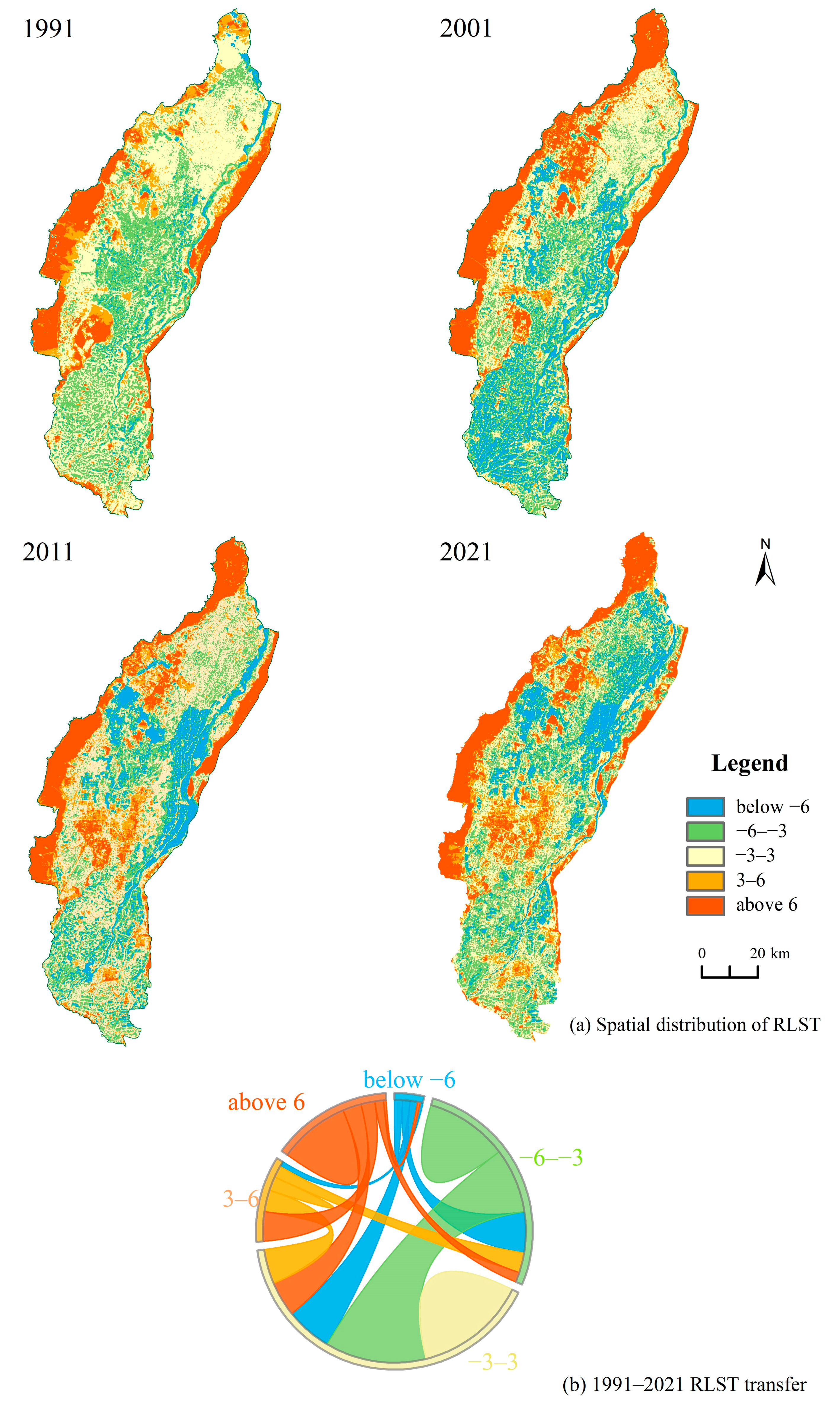
The RLST (Figure 2a) was calculated according to Equation (1). In the past 30 years, the thermal environment has been high in the east and west and low in the central area and the south. With the continuous expansion of built-up areas in the urbanization process, areas with high temperatures continues to increase, and great changes have occurred in the thermal environment spatial pattern over the whole research area. The mesophilic zone in the study area has shrunk significantly over the last 30 years, accounting for 47.3% of the changed area. Sub-high temperatures and high temperatures show an increasing trend, especially in the high-temperature area, with a growth rate of 29%.
Figure 2b shows the result of different grades of the RLST area transfer from 1991 to 2021: in 1991, the areas converted from a low temperature, sub-low temperature, and medium temperature to a high temperature were 25.958 km2, 90.826 km2, and 320.179 km2, totaling 436.963 km2 and accounting for 32.2% of the total area of change. The area converted from sub-high temperatures and high temperatures to low temperatures is 48.025 km2 and 23.462 km2, accounting for 7.6% of the total area of change. The increasing range and proportion of the RLST are significantly higher than those of a decreasing RLST, and the surface thermal environment shows a warming trend, which requires mitigation methods.
The contribution index of various land-use types to the thermal environment is calculated. As urbanization progresses, the obvious increase in built-up areas leads to an increase in spatial aggregation, which has a greater contribution to surface warming. The contribution of the built-up area to the regional thermal environment shows an obvious increasing trend, and the contribution of the built-up area to the surface thermal environment is close to 50% in 2021. The contribution of cultivated land and forestland to the surface thermal environment is relatively stable. Due to the small percentage of forestland, its contribution to the regional thermal environment is relatively small. The contributions of water, unused land, and grassland to the regional thermal environment first increased but then decreased. Several studies have found that water, grassland, forestland, and cultivated land have the effect of mitigating high surface temperatures, and these four heat sinks are classified as ecological land [22,48], while built-up areas and unused lands are classified as heat sources that raise the land’s surface temperature. Since ecological land contributes almost twice as much to cooling as nonecological land, it has a strong cooling effect.

4.1.2. Landscape Composition

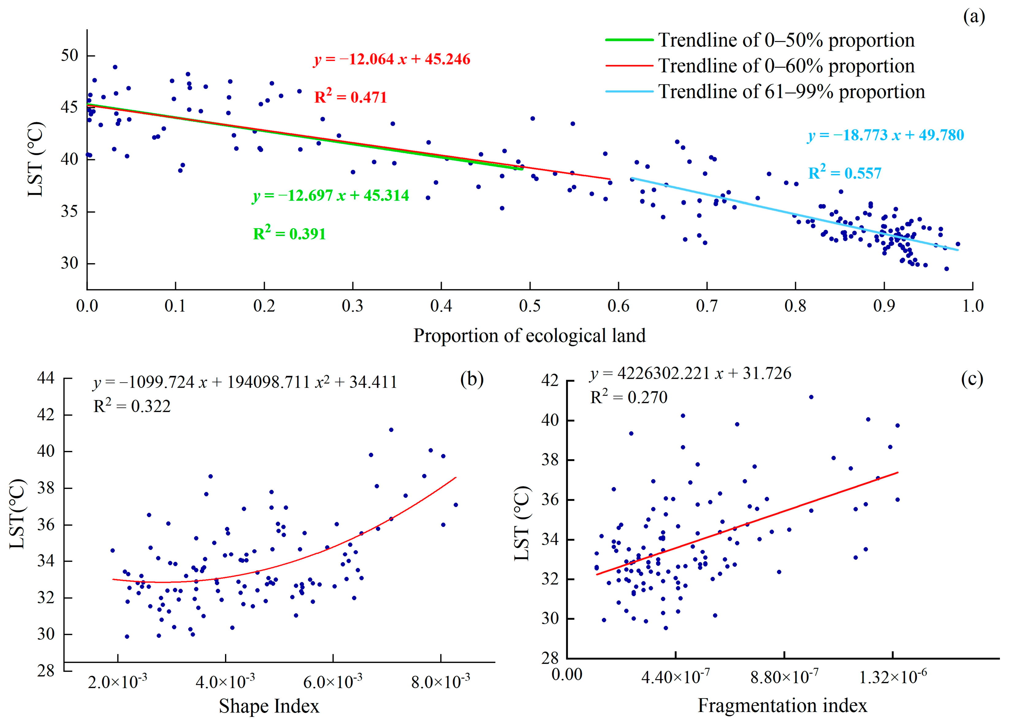
Ten grids with different lengths (the increment is 1.2 km, from 1.2 km to 12 km) were used to divide the study area, among which the 6 × 6 km grid was the best. Based on this scale, the fitting relationship between the area ratio of ecological land and surface temperature in 2021 was analyzed, and the results are shown in Figure 3. Overall, the area ratio of ecological land is negatively correlated with the LST; the higher the area ratio of ecological land, the lower the RLST. The threshold of ecological land with the greatest cooling effect was identified using a segmented linear regression. Using 10% as a step, the model fit coefficients were analyzed when the ratio of ecological land was in the range of 10–80%, and the results showed that the fit coefficients increased as the area ratio of ecological land increased. The R2 of the fitted model was 0.391 when the area ratio of ecological land reached 50% (p < 0.05), and the R2 increased to 0.471 when the area ratio of ecological land reached 60% (p < 0.05). Thus, the 61–99% area ratio interval of ecological land was selected for segmented fitting, and the R2 of the fitted model was improved to 0.557 (p < 0.05). In addition, fitting analyses were also performed using other area ratios of ecological lands as threshold inflection points, and the results were all lower than the corresponding results for the 61% threshold (see the Discussion section). Therefore, 61% was determined to be the threshold for the most significant cooling effect, corresponding to an area of approximately 21.6 km2. When the ecological land area ratio exceeded 61%, the cooling efficiency increased by 1.88°C for every 10% increase in the ecological land area ratio (R2 = 0.557, p < 0.05).

4.1.3. Landscape Configuration

Based on the threshold of the ecological land proportion, the data with an ecological land proportion greater than 61% were selected from the 6 × 6 km grid as the data source; the fragmentation index and shape index were calculated; and the fitting relationship between the index and the LST was analyzed. Figure 3b,c depicts the fitting analysis results. Both indices are positively correlated with the LST, and the LST increases as the index value increases. This finding indicates that those areas with more complex or fragmented ecological lands correspond to higher LSTs. In the fitting results of the two indices and the LST, the shape index was better than the fragmentation index, and the R2 was 0.322 (p < 0.05). The results show that the effect of landscape composition on the LST is stronger than that of spatial configuration. The degree of influence of the three types of factors on the LST was ranked from the largest to smallest as follows: ecological land proportion > shape index > fragmentation index.
In addition, a multiple linear regression analysis was performed by combining the three types of factors (Table 1). The best results are obtained when the area ratio of ecological land is >61%, both the shape index and fragmentation index are included in the modeling, and the fitted equation is y = 17.670 x 1 303.445 x 2 + 2230262.173 x 3 + 49.078 , where x 1 , x 2 , and x 3 are the area ratio of ecological land, shape index, and fragmentation index, respectively. The results indicate that when calculating the cooling effect of ecological land, the area ratio of ecological land should be considered first, and that simpler shapes and lower fragmentation are more conducive to reducing surface high temperatures.

4.2. Blocking the Heat Source Flow: Where Are the Patches and Corridors?

4.2.1. MSPA Classification and Connectivity

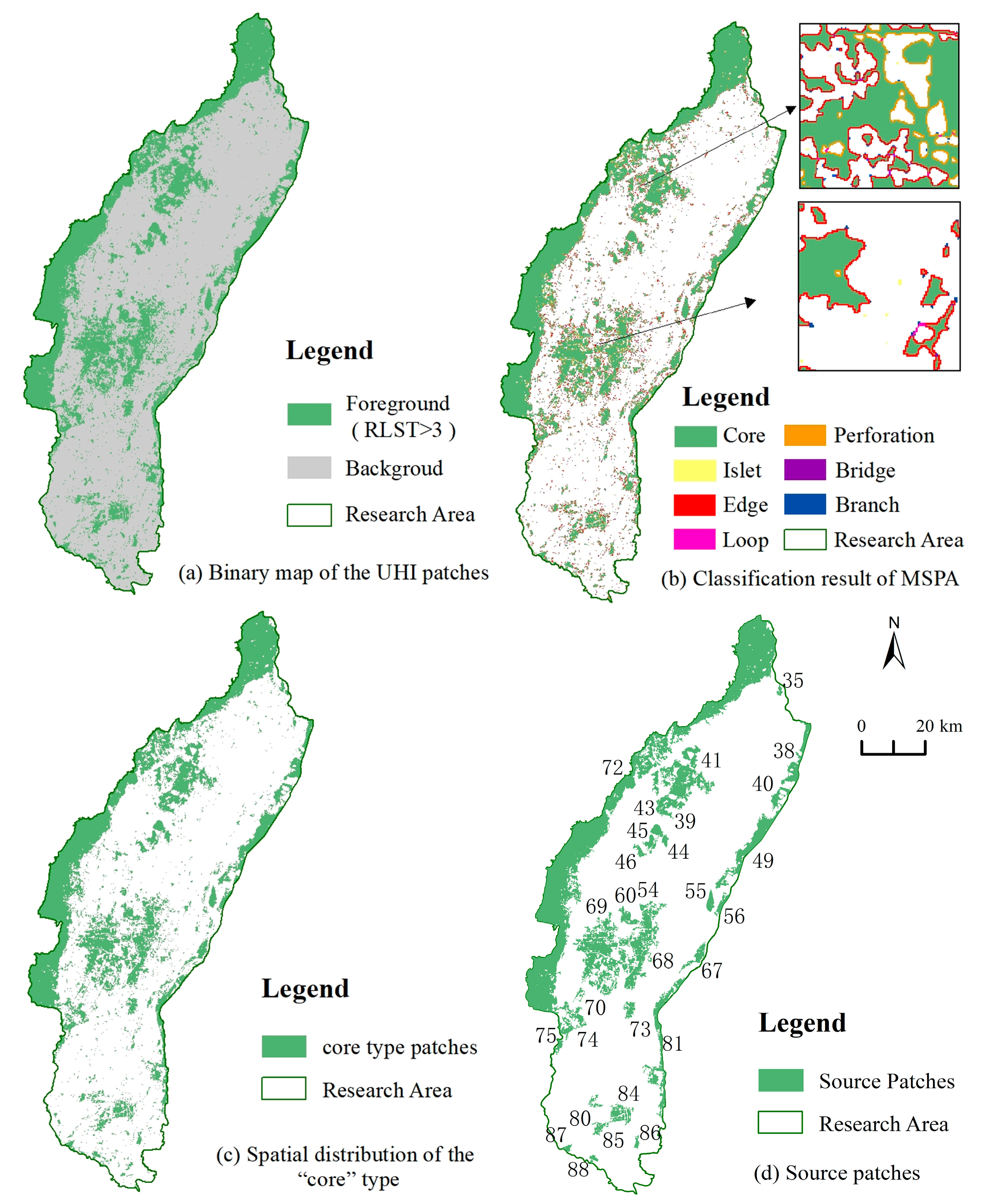
Figure 4b shows the results of the MSPA classification, where the core class has the highest number and area (Figure 4c): the number is 2795, accounting for 88.04% of the number of foreground patches and 26.58% of the total number of patches in the study area. The area is 1880.40 km2, accounting for 88.31% of the total study area. The spatial positions of the core area and the construction land and unused land are highly overlapping. The edge type is located outside the core, and its number accounts for 8.89% and 2.68% of the patches in the foreground and study area, respectively, and 8.73% of the foreground area. Perforation and branch accounted for a relatively low percentage of 1.99% and 0.67% of the number of foreground patches, respectively. Islets, rings, and bridges accounted for the lowest percentage of the MSPA category, all less than 0.4% (Table 2).
The core type is a significant feature of network stability in graph theory. In this study, the connectivity of the heat network (surface thermal environment) was measured by the core patches. Table 3 shows the top 30 index values of the connectivity of the core patches. The higher the connectivity, the faster the circulation of the thermal environment and the easier it is to spread, so they are selected as the diffusion source of the thermal environment (Figure 4d).

4.2.2. Resistance Surface

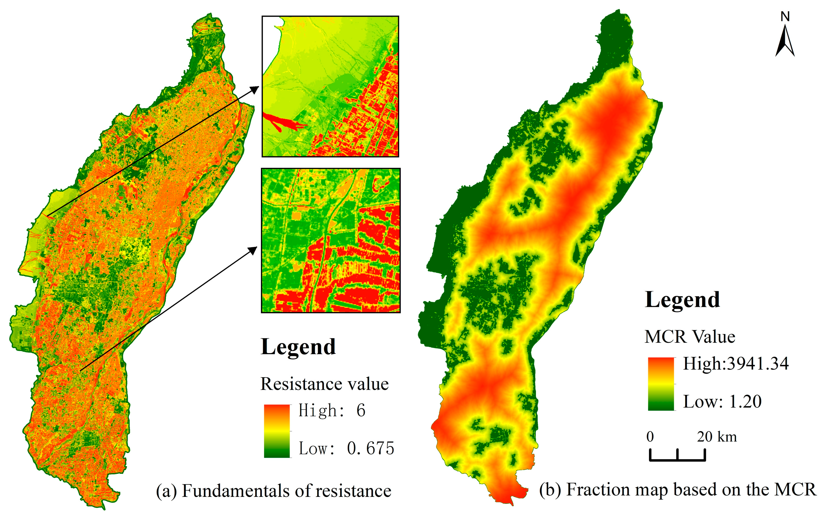
The comprehensive resistance surface (Figure 5a) is constructed by three types of factors: LUCC, DEM, and FVC, and the resistance values range from 0.675–6. Ecological land types, including vegetation and water, make up the majority of the surface coverage types in high-value locations, and the surface coverage types in low-value areas are mainly in built-up areas and unused land. The thermal resistance surface is established based on MCR, and the thermal resistance value ranges from 1.20–3941.34 (Figure 5b). The areas with high resistance values are mainly distributed in the north-central and southern parts of the study area, with the cultivated land and forestland widely distributed in the central-north area, and the cultivated land and grassland in the southern region, with only a small distribution of built-up areas. Overall, the resistance distribution rules of the minimum cumulative resistance surface and the comprehensive resistance surface are consistent, and the corresponding relationship between the resistance value and the surface cover type is also similar.

4.2.3. Corridors and Pinch Points of Heat Networks

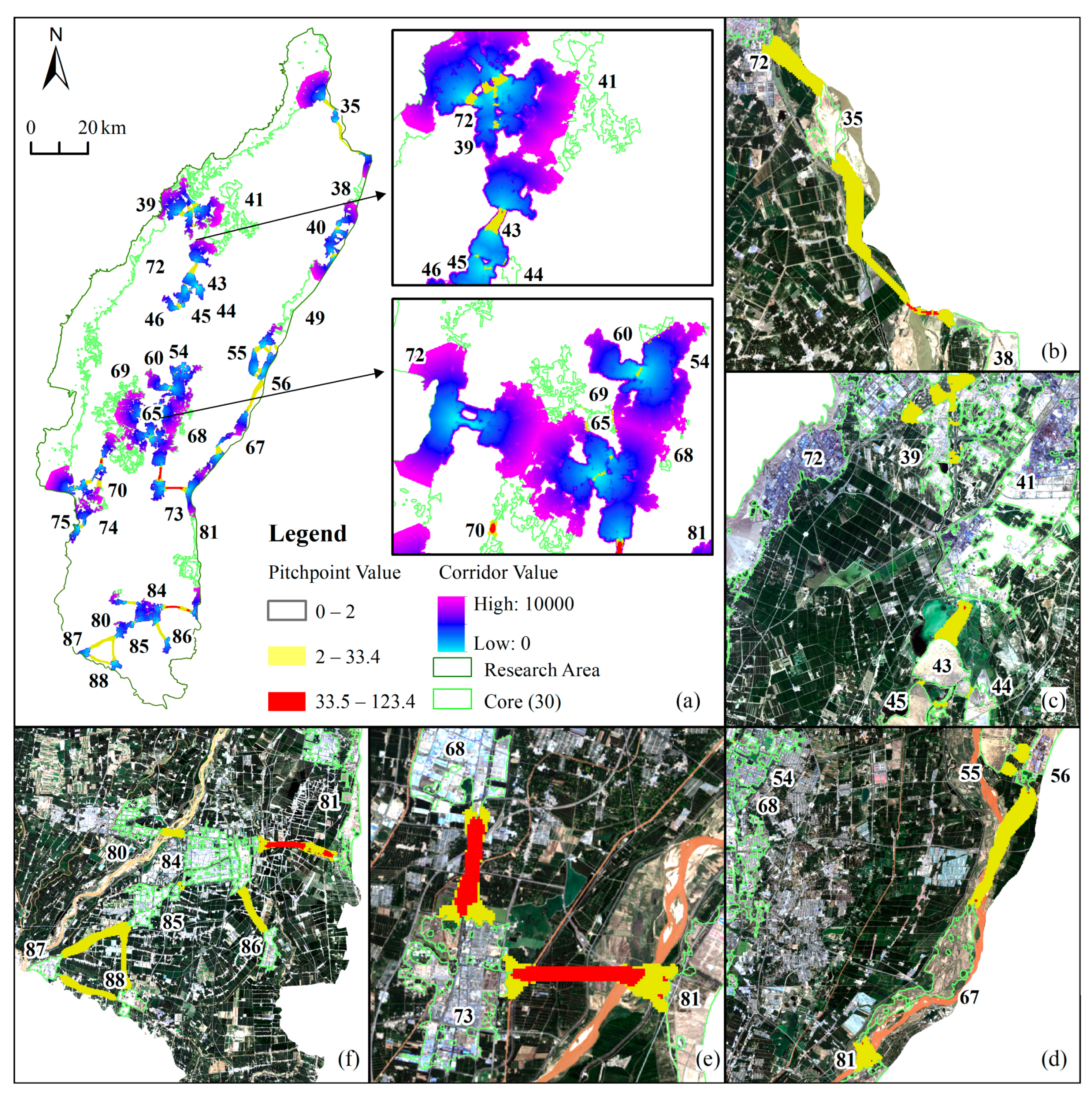
The top 30 patches of the connectivity value are selected as the source. Based on the source patch and resistance surface, a total of 34 corridors and 44 pinch points are extracted (Figure 6). The corridor is a narrow connecting channel between the source patches, and the smaller source patches are almost completely covered by the corridor, while the larger source patches are partially covered. The higher the effective resistance value of the corridor, the more difficult it is to connect with other patches, and the lower the effective resistance value, the easier it is to connect with other source patches. A corridor may contain multiple pinch points, and the pinch points are areas in the corridor where the heat flow is most concentrated. According to the classification of the effective resistance value, the pinch points are divided into three categories: general strength pinch points; medium strength pinch points, mainly distributed between built-up areas; and strong pinch points, mainly distributed between built-up areas and unused land (bare land, Gobi).
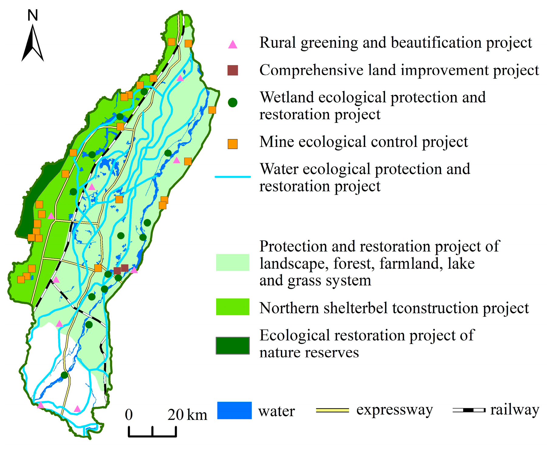
To confirm the rationality of the corridors and pinch points, this paper compares the data published by government departments, such as the Land Greening and Wetland Protection and Restoration Plan of the Ningxia Section of the Yellow River Basin and Special Plan for Ecological Protection and Restoration of Helan Mountain. These government programs are designed to make ecological improvements, enhance the livability of cities, and minimize ecological environmental problems, including the heat island effect. The key ecological environment improvement projects (Figure 7) involved in planning include the protection and restoration of wetlands along the Yellow River, the construction of natural or urban wetland parks, the reconstruction or construction of shelter forest systems along the mainstream of the Yellow River and around urban farmlands, and the ecological restoration of the Helan Mountain. After comparison and verification, the extracted pinch point is highly consistent with the deployment position of ecological land guided by planning; for example, the pinch point between the source patches (56–67, 73–81) along the Yellow River, the pinch point between the source patches (74–75) around Helan Mountain, and the pinch point between the source patches (41–43) of riverside parks in the built-up areas. It can support the reliability of the pinch point location analysis and provide effective decision support for planners.

4.3. Cooling Effect

Based on the premise that ecological land can be deployed within the pinch point (by adding new ecological land or enhancing the cooling effect of the original ecological land, etc.), we superimposed the pinch point with a grid with a side length of 6 × 6 km to estimate the cooling effect after deploying ecological land. According to the fitting results between the area ratio of ecological land and the LST, 61% is the most significant threshold for the cooling effect.
When the area ratio of ecological land is less than 61%, every 10% increase in the area ratio of ecological land will reduce the temperature by 1.20 °C. When the area ratio of ecological land is greater than 61%, every 10% increase in the area ratio of ecological land will reduce the temperature by 1.88 °C. Figure 8 shows the LST of 54 grids before and after cooling. The cooling range is between 0.04 °C and 6.02 °C, and the average temperature drop is 2.16 °C.

5. Discussion

5.1. The Rationality of the Research Method

From identifying the key points and deploying ecological land to estimating the cooling effects, this study proposes a complete and logical network. The entire analytical process includes numerous key methodological steps, the rationality of which has a significant impact on the results.
Graph theory, which analyzes the connectivity of complex landscape patterns as a kind of network, has received widespread usage in research on biodiversity, biological conservation, ecological pattern security, etc. The spreading mode of the surface thermal environment is dynamic and random, and the morphological image-processing method is also appropriate for a surface thermal landscape analysis. Therefore, the MSPA model is used to classify the thermal landscape. According to the RLST, the surface heating network is established, and the core patches that may cause surface temperature rises are located. The importance of the core patches is graded according to the connectivity index, and the source patches of the surface temperature are identified.
The random spreading characteristics of the thermal patches are similar to those of currents. Based on the MCR model, a thermal resistance surface is established to describe the resistance of the thermal environment when it expands in a complex landscape pattern. Combined with circuit theory, resistance surfaces and source patches are used to determine the corridors and pinch points in the thermal network and their effective resistance values.
The area ratio, shape, and fragmentation of ecological land all have a significant impact on the regional thermal environment. A correlation analysis, multiple linear regression methods, and a piecewise linear regression were used to investigate the impact of three types of factors on the thermal environment, identify the most significant factors influencing the cooling effect of ecological land, and define the cooling effect threshold, which has a certain guiding significance for the deployment of ecological land. The above simulation relationship is used to estimate the cooling effect after deploying ecological land. Based on the case study findings, the method chosen for this study is highly adaptable to the analytical process and can meet the research requirements.

5.2. Applicability of the Research Process to Cooling Surface Thermal Environments

The UHI effect has had a negative impact on the ecological environment and human beings [49], and it is necessary to mitigate the land’s high temperature. Most previous studies have been analyzed from a single point of view, and some of them analyzed the factor that has the greatest impact among the many factors that lead to surface warming [11]. Some discussed the influence of the size, shape, fragmentation, and other characteristics [50,51] of the patch on the surface temperature in terms of the patch. Some researchers have discussed the cooling effect of the blue-green surface type ratio [52]. However, opinions from a single point of view are of limited help in achieving the actual surface cooling; for example, the inability to determine where to deploy governance. In practice, it is difficult to develop a systematic mitigation strategy [24], and it is impossible to present a systematic inspiration plan for reducing high surface temperatures [25,29]. The mitigation of a surface high temperature is a complex analysis process, which cannot be solved by only a single aspect of research and analysis. It requires a systematic and coherent research logic network. This research proposes a relatively complete research process. Taking the Yinchuan metropolitan region as a case study, 44 pinch points were identified in 34 thermal corridors, and 54 ecological lands were selected for grid deployment. The cooling range was between 0.04 °C and 6.02 °C, with an average cooling of 2.16 °C. The results show that in the system of mitigating the surface temperature, we should first pay attention to the key corridors and pinch points of heat circulation and build ecological land with an area ratio close to the cooling threshold (simple shape and low fragmentation). Overall, this research case serves as a reference for mitigating thermal environments and improving the sustainable development of cities (regions).

5.3. Factors Influencing the Simulation

5.3.1. Impact of Grid Size on the Fitted Relationship

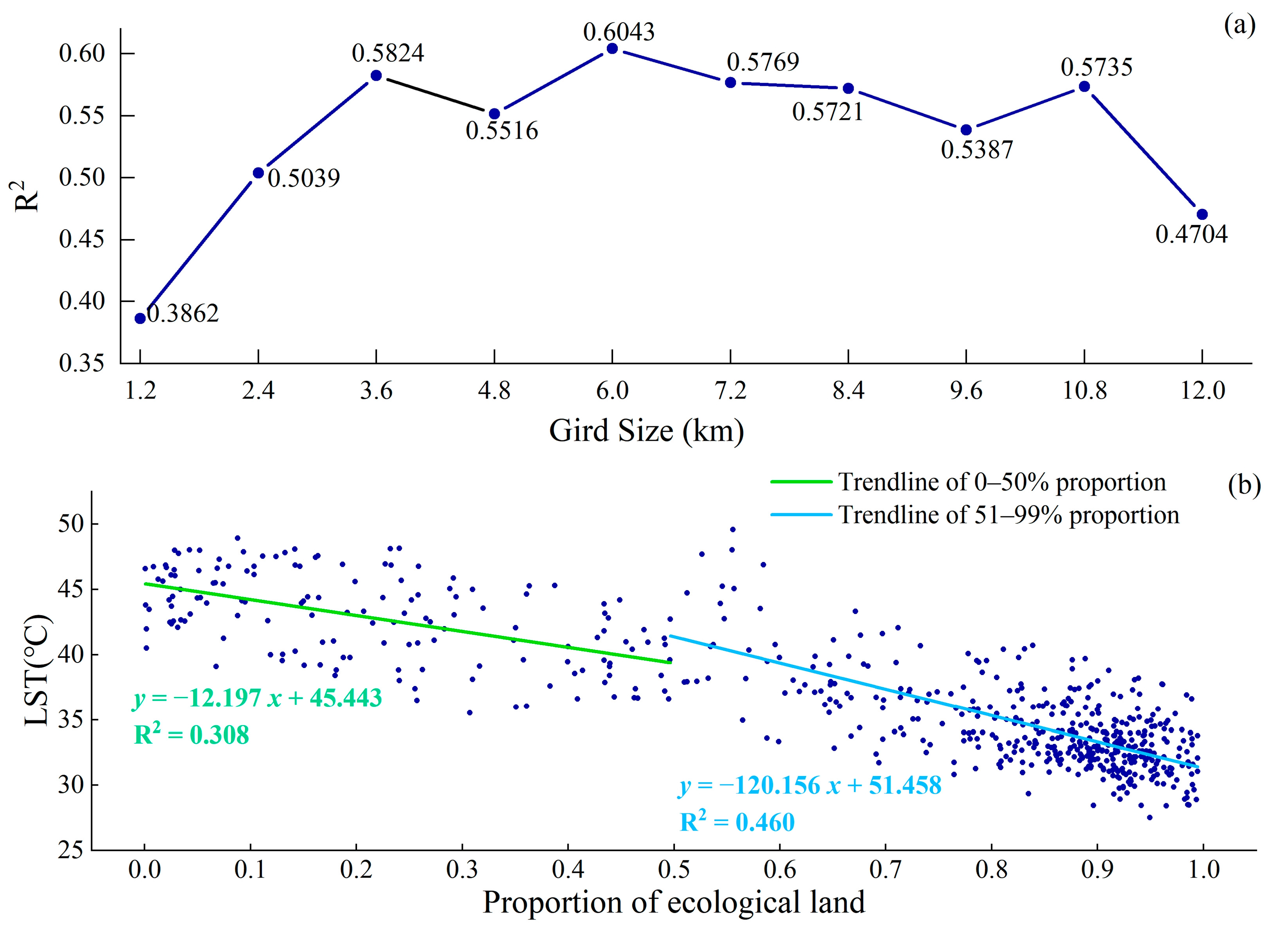
The grid is divided to determine the area ratio of ecological land, shape index, and fragmentation index within a given range. The following considerations should be made when determining the grid threshold: (1) The study area is approximately 7072 km2, and the grid size should not be excessively large or small. (2) Because the pixels in the Landsat OLI image are 30 × 30 m, the grid size should be an integer multiple of 30. (3) The appropriate edge length of the grid is selected based on the fitting effect of each variable with LST. In the experiment, the fitting effects of 10 kinds of grids are tested in increments of 1.2 km from 1.2 km to 12 km, with comparisons and analyses from two aspects. Figure 9a is the fitting result of the ecological land area ratio and the LST (different grid sizes). With the increase in grid size, the fitting coefficient (R2) between the LST and the ecological land area ratio increases. R2 is greater than 0.5 when the grid size ranges from 2.4 km to 10.8 km, indicating a fluctuating state. When the grid size is 6 km, the highest R2 is 0.6043 (p < 0.05). The fitting effect is relatively low when the grid size is 1.2 km and 12 km, suggesting that the length is too large or too small, which is not conducive to the objective presentation of the research results.
When the grid size is 3.6 km, the fitting result is second only to that when the grid size is 6 km. By analyzing the ecological land proportion threshold of the 3.6 km grid, it appears at approximately 50% (Figure 9b), which is close to the threshold of the ecological land-use ratio (61%) of the 6 km grid, indicating that the selection of the threshold of the ecological land-use ratio is reasonable.

5.3.2. Factors and Coefficients for Constructing the Resistance Surface

Varied land types exhibit distinctly different solar radiation reflection and absorption properties. Urban impervious surfaces, such as built-up areas and unused land, exhibit higher temperatures. Since vegetation and water bodies can absorb more solar radiation, the temperature of such features is lower and their cooling effect on the surrounding landscape decreases with an increasing distance. In areas with large differences in surface elevation, the vertical temperature gradient is also a factor that affects the surface temperature. Four main factors were considered in constructing the resistance surface, including the LUCC, DEM, FVC, and distance from water.
  • The single-factor resistance value
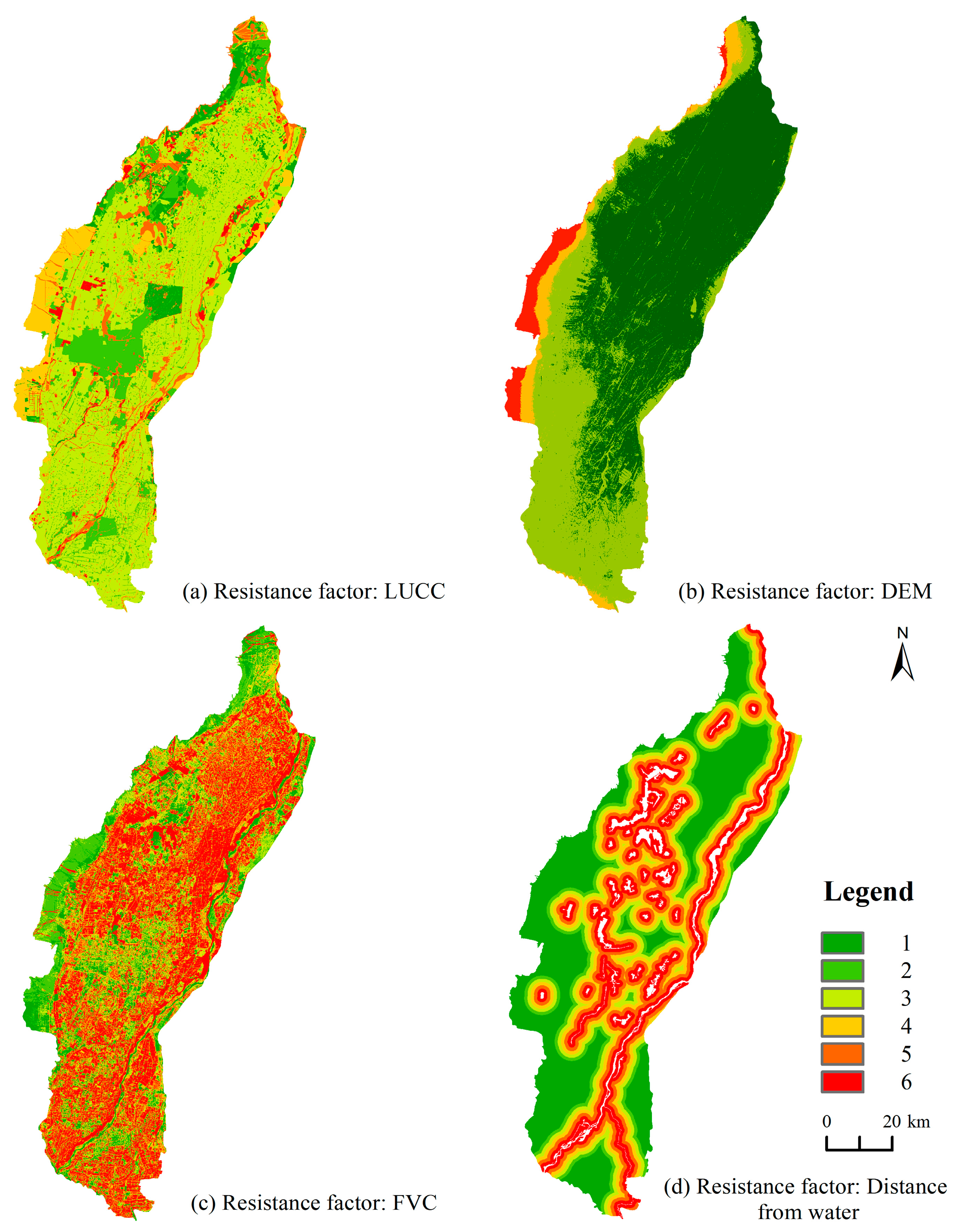
Vegetation, water, and other ecological lands have a cooling effect, which has great resistance to the spread of the surface thermal environment. Construction land and unused land (mostly bare land) have higher surface temperatures and less resistance to the spread of the surface thermal environment. The area with a higher FVC has a cooler surface temperature, and the region closer to the water has a cooler surface temperature. Factors that promote the diffusion of heat sources were assigned lower resistance values, and factors that hinder the diffusion of heat sources were assigned higher resistance values (Figure 10). Considering the reasonableness of the classification of the four categories of factors (LUCC, DEM, FVC, and distance from water), the quantile classification method was used to classify the resistance [53] from low to high into six levels, labeled 1, 2, 3, 4, 5, and 6, respectively (Table 4).
2.
Total resistance value
The dependent variable is the RLST, and the independent variables are the LUCC, FVC, DEM, and distance from water. The correlation coefficient between the dependent variable and the independent variable is calculated by the geographic detector [54]. The geographic detector is a statistical model that measures the driving force of spatially stratified heterogeneity exploration, and this method was used to detect the spatially heterogeneous influence of the independent variable on the surface thermal environment. The q value represents the degree of explanation; q takes the value interval [0,1], and a q value closer to one represents the stronger explanatory power of the independent variable on the RLST. The q values of the FVC, LUCC, DEM, and distance from water are 0.503, 0.338, 0.198, and 0.007, respectively, and their p values are all less than 0.005. The correlation between the RLST and distance from water is weak, so this factor is abandoned. The correlation coefficient is normalized, and the total resistance coefficients of the FVC, LUCC, and DEM are 0.484, 0.325, and 0.191, respectively.

5.3.3. Resistance Threshold of the Corridor

The corridor is a crucial pathway for the thermal environment to spread, and indeed, the width of the corridor has an apparent impact on the heat flow. The corridor area was calculated by setting five cumulative resistance thresholds ranging from 2 k to 18 k in 4 k increments, and the proportion of the corridor area to the source patch area was 6.59%, 30.84%, 54.89%, 76.11%, and 91.70%. The area of the corridor expands as the cumulative resistance threshold increases, but the spatial position remains essentially unchanged. With the increasing corridor width, the heat flow is diverted, and the maximum accumulated current of the pinch point decreases; however, the spatial distribution of the pinch points does not obviously change, indicating that the threshold has little influence on the spatial position of the pinch point and that the pinch point is effective in cooling the thermal environment. In this case, the pinch point’s location is compared to the ecological governance location mentioned in planning documents, such as ecological governance in the study area, and 10 k is used as the threshold to calculate the corridor and the pinch point.

5.4. Limitations and Future Study

The accuracy of the basic data used in the research (LST, LUCC, FVC, etc.) has a direct impact on the analytical results. The research area is 7072 km2, and the basic data accuracy is well-matched with the analysis results. However, when the study area is small, it is necessary to improve the basic data interpretation ability, particularly the boundary segmentation accuracy of the source patch, to obtain more accurate analytical results.
In reality, some areas within the pinch point may be unable to add new ecological land. To reduce the surface temperature, we can consider increasing the cooling effect of the in situ type. The in situ type, for example, is sparse grassland, which can promote cooling by increasing vegetation richness. The in situ type is the riparian tidal flat, which can improve the ecological function of the river channel and promote cooling by creating a riverside landscape green space. Therefore, simulating the cooling effect has some limitations that can be evaluated in conjunction with more detailed planning data in actual work.
When constructing the resistance surface and analyzing the landscape composition or landscape index for the evaluation of the cooling effect of ecological land, it is recommended to add analysis factors with high suitability in the study area to further enhance their local suitability.

6. Conclusions

With climate change and urbanization processes, the UHI effect imposes increasingly serious harm on human beings and the ecosystem. Ecological land with a cooling function can be used to mitigate the thermal environment and help maintain a good ecological quality and improve human living comfort. We integrated both patch and network perspectives to cool the surface thermal environment through the rational allocation of ecological land. Using the Yinchuan metropolitan region as an example, we propose locating the pinch points and deploying suitable ecological land for them, blocking connectivity between thermal patches, effectively preventing the formation of a larger thermal network due to thermal patch connectivity, and estimating the regional cooling effect. The fitting precision of landscape factors and surface temperature is described as follows: area ratio of ecological land > shape index > fragmentation index. Next, 61% was the most significant threshold of the area ratio of ecological land, and when it exceeded 61%, the cooling efficiency increased by 1.88°C for every 10% rise in the ecological land area ratio (R2 = 0.557, p < 0.05). The study area was divided into seven types based on the MSPA classification, with core patches accounting for the greatest number and area, with 88.04% of the number of foreground patches and 88.31% of the total area. Selecting the patches with the top 30 connectivity index values as the heat source and combining them with the heat resistance surface calculated by the MCR model, 34 corridors and 44 pinch points are identified based on circuit theory. After the deployment of ecological land, the cooling range of 54 grids is between 0.04 °C and 6.02 °C, with an average cooling of 2.16 °C. Priority should be given to pinch points and corridor areas when implementing surface temperature cooling measures.
This research case offers new ideas for cooling the thermal environment and enhancing cities’ sustainability performance, particularly in the context of the Yellow River basin’s national strategy for high-quality development, and it provides a reference for improving the ecological environment quality in arid and semiarid areas.

Author Contributions

Writing—original draft, D.W.; writing—review and editing, H.S.; funding acquisition, D.W. and H.S.; methodology, D.W., H.S., H.X. and Z.X.; investigation, T.Z.; visualization, D.W., H.X., Z.X. and L.W.; software, D.W., H.X., T.Z. and Z.X.; data curation, L.W. All authors have read and agreed to the published version of the manuscript.

Funding

This research was funded by the Natural Science Foundation of the Ningxia Hui Autonomous Region (Grant No. 2021AAC03456), the Ningxia Hui Autonomous Region Excellent Talents Support Program, the Ningxia Hui Autonomous Region Key Research and Development Program (Grant No. 2022BEG03064), the Beijing Municipal Natural Science Foundation (Grant No. 6222045), the National Natural Science Foundation of China (Grant No. 41871338), and the Fundamental Research Funds for the Central Universities.

Data Availability Statement

Not applicable.

Acknowledgments

We give special thanks to the guidance and suggestions of the research group of Hao Sun, from the College of Geoscience and Surveying Engineering, China University of Mining and Technology-Beijing. Additionally, we gratefully acknowledge the anonymous reviewers’ constructive comments and the editor’s efforts to improve this manuscript.

Conflicts of Interest

The authors declare no conflict of interest.

References

  1. Sheng, S.; Xiao, H.; Wang, Y. The cooling effects of hybrid landscapes at the district scale in mega-cities: A case study of Shanghai. J. Cleaner Prod. 2022, 366, 132942. [Google Scholar] [CrossRef]
  2. Khare, V.R.; Vajpai, A.; Gupta, D. A big picture of urban heat island mitigation strategies and recommendation for India. Urban Clim. 2021, 37, 100845. [Google Scholar] [CrossRef]
  3. Huang, A.; Shen, R.; Jia, G.; Xu, X. Reforestation enhanced landscape connectivity for thermal buffering in China. Environ. Res. Lett. 2022, 17, 014056. [Google Scholar] [CrossRef]
  4. Hyseni, C.; Heino, J.; Bini, L.M.; Bjelke, U.; Johansson, F. The importance of blue and green landscape connectivity for biodiversity in urban ponds. Basic Appl. Ecol. 2021, 57, 129–145. [Google Scholar] [CrossRef]
  5. Peng, J.; Cheng, X.; Hu, Y.; Corcoran, J. A landscape connectivity approach to mitigating the urban heat island effect. Landsc. Ecol. 2022, 37, 1707–1719. [Google Scholar] [CrossRef]
  6. Zou, Z.; Yan, C.; Yu, L.; Jiang, X.; Ding, J.; Qin, L.; Wang, B.; Qiu, G. Impacts of land use/ land cover types on interactions between urban heat island effects and heat waves. Build. Environ. 2021, 204, 108138. [Google Scholar] [CrossRef]
  7. Tran, D.X.; Pla, F.; Latorre-Carmona, P.; Myint, S.W.; Gaetano, M.; Kieu, H.V. Characterizing the relationship between land use land cover change and land surface temperature. ISPRS J. Photogramm. Remote Sens. 2017, 124, 119–132. [Google Scholar] [CrossRef] [Green Version]
  8. Lai, D.; Liu, W.; Gan, T.; Liu, K.; Chen, Q. A review of mitigating strategies to improve the thermal environment and thermal comfort in urban outdoor spaces. Sci. Total Environ. 2019, 661, 337–353. [Google Scholar] [CrossRef]
  9. Yu, Z.; Yang, G.; Zuo, S.; Jorgensen, G.; Koga, M.; Vejre, H. Critical review on the cooling effect of urban blue-green space: A threshold-size perspective. Urban For. Urban Green. 2020, 49, 126630. [Google Scholar] [CrossRef]
  10. Xu, C.; Chen, G.; Huang, Q.; Su, M.; Rong, Q.; Yue, W.; Haase, D. Can improving the spatial equity of urban green space mitigate the effect of urban heat islands? An empirical study. Sci. Total Environ. 2022, 841, 156687. [Google Scholar] [CrossRef]
  11. Tan, M.; Li, X. Integrated assessment of the cool island intensity of green spaces in the mega city of Beijing. Int. J. Remote Sens. 2013, 34, 3028–3043. [Google Scholar] [CrossRef]
  12. Peng, J.; Xie, P.; Liu, Y.; Ma, J. Urban thermal environment dynamics and associated landscape pattern factors: A case study in the Beijing metropolitan region. Remote Sens. Environ. 2016, 173, 145–155. [Google Scholar] [CrossRef]
  13. Zhang, C.; Wu, J.; Grimm, N.B.; McHale, M.; Buyantuyev, A. A hierarchical patch mosaic ecosystem model for urban landscapes: Model development and evaluation. Ecol. Model. 2013, 250, 81–100. [Google Scholar] [CrossRef]
  14. Zhou, W.; Qian, Y.; Li, X.; Li, W.; Han, L. Relationships between land cover and the surface urban heat island: Seasonal variability and effects of spatial and thematic resolution of land cover data on predicting land surface temperatures. Landsc. Ecol. 2014, 29, 153–167. [Google Scholar] [CrossRef]
  15. Ke, X.; Men, H.; Zhou, T.; Li, Z.; Zhu, F. Variance of the impact of urban green space on the urban heat island effect among different urban functional zones: A case study in Wuhan. Urban For. Urban Green. 2021, 62, 127159. [Google Scholar] [CrossRef]
  16. Zhou, W.; Yu, W.; Wu, T. An alternative method of developing landscape strategies for urban cooling: A threshold-based perspective. Landsc. Urban Plann. 2022, 225, 104449. [Google Scholar] [CrossRef]
  17. Xia, H.; Chen, Y.; Song, C.; Li, J.; Quan, J.; Zhou, G. Analysis of surface urban heat islands based on local climate zones via spatiotemporally enhanced land surface temperature. Remote Sens. Environ. 2022, 273, 112972. [Google Scholar] [CrossRef]
  18. Zhou, Y.; Gao, W.; Yang, C.; Shen, Y. Exploratory analysis of the influence of landscape patterns on lake cooling effect in Wuhan, China. Urban Clim. 2021, 39, 100969. [Google Scholar] [CrossRef]
  19. Cui, L.; Wang, J.; Sun, L.; Lv, C. Construction and optimization of green space ecological networks in urban fringe areas: A case study with the urban fringe area of Tongzhou district in Beijing. J. Cleaner Prod. 2020, 276, 124266. [Google Scholar] [CrossRef]
  20. Zhang, Z.; Meerow, S.; Newell, J.P.; Lindquist, M. Enhancing landscape connectivity through multifunctional green infrastructure corridor modeling and design. Urban For. Urban Green. 2019, 38, 305–317. [Google Scholar] [CrossRef]
  21. Peng, J.; Hu, Y.; Dong, J.; Liu, Q.; Liu, Y. Quantifying spatial morphology and connectivity of urban heat islands in a megacity: A radius approach. Sci. Total Environ. 2020, 714, 136792. [Google Scholar] [CrossRef] [PubMed]
  22. Yu, Z.; Yao, Y.; Yang, G.; Wang, X.; Vejre, H. Strong contribution of rapid urbanization and urban agglomeration development to regional thermal environment dynamics and evolution. For. Ecol. Manag. 2019, 446, 214–225. [Google Scholar] [CrossRef]
  23. Grafius, D.R.; Corstanje, R.; Siriwardena, G.M.; Plummer, K.E.; Harris, J.A. A bird’s eye view: Using circuit theory to study urban landscape connectivity for birds. Landsc. Ecol. 2017, 32, 1771–1787. [Google Scholar] [CrossRef] [PubMed] [Green Version]
  24. Yu, Z.; Zhang, J.; Yang, G. How to build a heat network to alleviate surface heat island effect? Sus. Cities Soc. 2021, 74, 103135. [Google Scholar] [CrossRef]
  25. Yu, Z.; Zhang, J.; Yang, G.; Schlaberg, J. Reverse Thinking: A New Method from the Graph Perspective for Evaluating and Mitigating Regional Surface Heat Islands. Remote Sens. 2021, 13, 1127. [Google Scholar] [CrossRef]
  26. Liu, Q.; Xie, M.; Wu, R.; Xue, Q.; Chen, B.; Li, Z.; Li, X. From expanding areas to stable areas: Identification, classification and determinants of multiple frequency urban heat islands. Ecol. Indic. 2021, 130, 108046. [Google Scholar] [CrossRef]
  27. Xie, M.; Gao, Y.; Cao, Y.; Breuste, J.; Fu, M.; Tong, D. Dynamics and Temperature Regulation Function of Urban Green Connectivity. J. Urban Plann. Dev. 2015, 141, A5014008. [Google Scholar] [CrossRef]
  28. Lian, Z.; Feng, X. Urban Green Space Pattern in Core Cities of the Greater Bay Area Based on Morphological Spatial Pattern Analysis. Sustainability 2022, 14, 12365. [Google Scholar] [CrossRef]
  29. Mokhtari, Z.; Barghjelveh, S.; Sayahnia, R.; Karami, P.; Qureshi, S.; Russo, A. Spatial pattern of the green heat sink using patch- and network-based analysis: Implication for urban temperature alleviation. Sus. Cities Soc. 2022, 83, 103964. [Google Scholar] [CrossRef]
  30. Chen, L.; Sun, R.; Lu, Y. A conceptual model for a process-oriented landscape pattern analysis. Sci. China-Earth Sci. 2019, 62, 2050–2057. [Google Scholar] [CrossRef]
  31. Gao, J.; Gong, J.; Yang, J.; Li, J.; Li, S. Measuring Spatial Connectivity between patches of the heat source and sink (SCSS): A new index to quantify the heterogeneity impacts of landscape patterns on land surface temperature. Landsc. Urban Plann. 2022, 217, 104260. [Google Scholar] [CrossRef]
  32. Lyu, R.; Pang, J.; Tian, X.; Zhao, W.; Zhang, J. How to optimize the 2D/3D urban thermal environment: Insights derived from UAV LiDAR/multispectral data and multi-source remote sensing data. Sus. Cities Soc. 2023, 88, 104287. [Google Scholar] [CrossRef]
  33. Yuan, F.; Bauer, M.E. Comparison of impervious surface area and normalized difference vegetation index as indicators of surface urban heat island effects in Landsat imagery. Remote Sens. Environ. 2007, 106, 375–386. [Google Scholar] [CrossRef]
  34. Li, K.; Chen, Y.; Gao, S. Comparative Analysis of Variations and Patterns between Surface Urban Heat Island Intensity and Frequency across 305 Chinese Cities. Remote Sens. 2021, 13, 3505. [Google Scholar] [CrossRef]
  35. Forestry and Grassland Bureau of Ningxia Hui Autonomous Region Home Page. Available online: http://lcj.nx.gov.cn/zwgk/zfxxgkml/ghxx/202112/t20211213_3219671.html (accessed on 20 January 2023).
  36. Department of Ecology and Environment of Ningxia Hui Autonomous Region Home Page. Available online: https://sthjt.nx.gov.cn/zwgk/hjgh/hhlystbh/202210/t20221031_3823687.html (accessed on 20 January 2023).
  37. People’s Government of Shizuishan City Home Page. Available online: http://www.shizuishan.gov.cn/zwgk/zc/szfwj/szbf/202204/t20220406_3418273.html (accessed on 20 January 2023).
  38. Haashemi, S.; Weng, Q.; Darvishi, A.; Alavipanah, S.K. Seasonal Variations of the Surface Urban Heat Island in a Semi-Arid City. Remote Sens. 2016, 8, 352. [Google Scholar] [CrossRef] [Green Version]
  39. Sun, R.; Chen, L. Effects of green space dynamics on urban heat islands: Mitigation and diversification. Ecosyst. Serv. 2017, 23, 38–46. [Google Scholar] [CrossRef]
  40. Peng, J.; Wang, Y.; Zhang, Y.; Wu, J.; Li, W.; Li, Y. Evaluating the effectiveness of landscape metrics in quantifying spatial patterns. Ecol. Indic. 2010, 10, 217–223. [Google Scholar] [CrossRef]
  41. An, Y.; Liu, S.; Sun, Y.; Shi, F.; Beazley, R. Construction and optimization of an ecological network based on morphological spatial pattern analysis and circuit theory. Landsc. Ecol. 2021, 36, 2059–2076. [Google Scholar] [CrossRef]
  42. Wickham, J.D.; Riitters, K.H.; Wade, T.G.; Vogt, P. A national assessment of green infrastructure and change for the conterminous United States using morphological image processing. Landsc. Urban Plann. 2010, 94, 186–195. [Google Scholar] [CrossRef]
  43. Saura, S.; Torné, J. Conefor Sensinode 2.2: A software package for quantifying the importance of habitat patches for landscape connectivity. Environ. Modell. Softw. 2009, 24, 135–139. [Google Scholar] [CrossRef]
  44. Dai, L.; Liu, Y.; Luo, X. Integrating the MCR and DOI models to construct an ecological security network for the urban agglomeration around Poyang Lake, China. Sci. Total Environ. 2021, 754, 141868. [Google Scholar] [CrossRef] [PubMed]
  45. Li, Y.-Y.; Zhang, Y.-Z.; Jiang, Z.-Y.; Guo, C.-X.; Zhao, M.-Y.; Yang, Z.-G.; Guo, M.-Y.; Wu, B.-Y.; Chen, Q.-L. Integrating morphological spatial pattern analysis and the minimal cumulative resistance model to optimize urban ecological networks: A case study in Shenzhen City, China. Ecol. Process. 2021, 10, 1–15. [Google Scholar] [CrossRef]
  46. Leonard, P.B.; Duffy, E.B.; Baldwin, R.F.; McRae, B.H.; Shah, V.B.; Mohapatra, T.K. gflow: Software for modeling circuit theory-based connectivity at any scale. Methods Ecol. Evol. 2017, 8, 519–526. [Google Scholar] [CrossRef] [Green Version]
  47. McRae, B.H.; Beier, P. Circuit theory predicts gene flow in plant and animal populations. Proc. Natl. Acad. Sci. USA 2007, 104, 19885–19890. [Google Scholar] [CrossRef] [Green Version]
  48. Feng, H.H.; Zhao, X.F.; Chen, F.; Wu, L.C. Using land use change trajectories to quantify the effects of urbanization on urban heat island. Adv. Space Res. 2014, 53, 463–473. [Google Scholar] [CrossRef]
  49. Hondula, D.M.; Vanos, J.K.; Gosling, S.N. The SSC: A decade of climate-health research and future directions. Int. J. Biometeorol. 2014, 58, 109–120. [Google Scholar] [CrossRef]
  50. Yang, L.; Niyogi, D.; Tewari, M.; Aliaga, D.; Chen, F.; Tian, F.; Ni, G. Contrasting impacts of urban forms on the future thermal environment: Example of Beijing metropolitan area. Environ. Res. Lett. 2016, 11, 034018. [Google Scholar] [CrossRef] [Green Version]
  51. Sun, Y.; Li, Y.; Ma, R.; Gao, C.; Wu, Y. Mapping urban socio-economic vulnerability related to heat risk: A grid-based assessment framework by combing the geospatial big data. Urban Clim. 2022, 43, 101169. [Google Scholar] [CrossRef]
  52. Fan, H.; Yu, Z.; Yang, G.; Liu, T.Y.; Liu, T.Y.; Hung, C.H.; Vejre, H. How to cool hot-humid (Asian) cities with urban trees? An optimal landscape size perspective. Agric. For. Meteorol. 2019, 265, 338–348. [Google Scholar] [CrossRef]
  53. Yu, Q.; Yue, D.P.; Wang, J.P.; Zhang, Q.B.; Li, Y.T.; Yu, Y.; Chen, J.X.; Li, N. The optimization of urban ecological infrastructure network based on the changes of county landscape patterns: A typical case study of ecological fragile zone located at Deng Kou (Inner Mongolia). J. Cleaner Prod. 2017, 163, S54–S67. [Google Scholar] [CrossRef]
  54. Wang, J.; Xu, C.; Hu, M.; Li, Q.; Yan, Z.; Jones, P. Global land surface air temperature dynamics since 1880. Int. J. Climatol. 2018, 38, 466–474. [Google Scholar] [CrossRef]
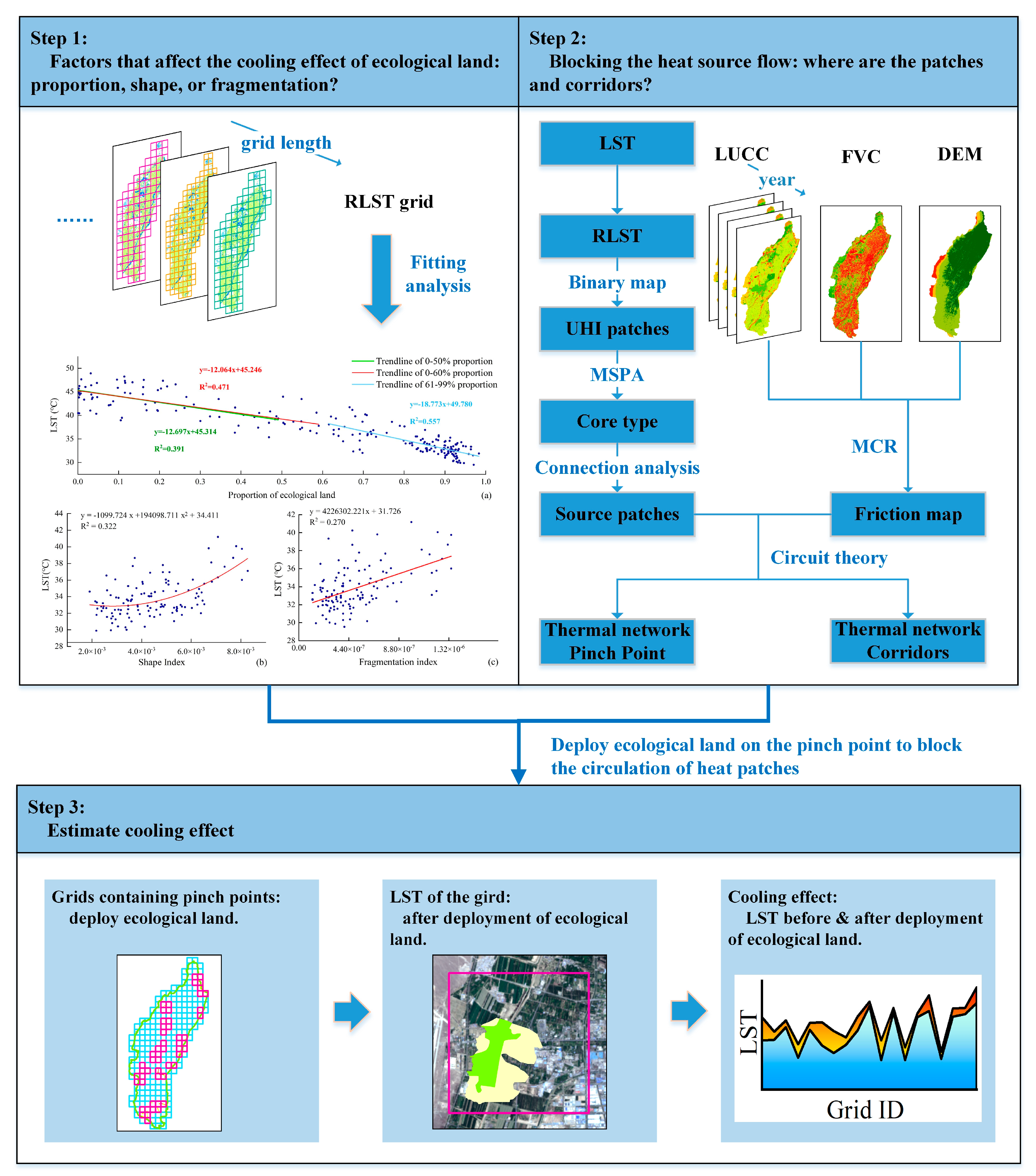
Figure 1. A comprehensive perspective analysis process of the patch and network for cooling surface thermal environment. There are three steps, which are as follows: (1) investigate the effects of landscape composition and spatial configuration on the surface thermal environment; (2) identify the network pinch points and corridors that prevent surface thermal environment circulation; and (3) deploy ecological land at the pinch points to block the connection between the heat patches and cool the surface temperature.
Remotesensing 15 01061 g001
Figure 2. Spatiotemporal pattern of and variation in RLST: (a) spatial distribution of RLST from 1991 to 2021; (b) transformation of RLST from 1991 to 2021. According to RLST, the heat island intensity is classified into 5 classes: −6 ≥ low, −6 < sub-low ≤ −3, −3 < medium ≤ 3, 3 < sub-high ≤ 6, and 6 < high.
Remotesensing 15 01061 g002
Figure 3. Analysis of the effects of 3 landscape composition factors (proportion, shape, or fragmentation) on LST: (a) A segmented linear regression method was used to fit the ecological land proportion with LST in steps of 10% to determine the ecological land threshold with the most significant cooling effect. (b) Fitting results of shape index and land surface temperature. (c) Fitting results of fragmentation index and land surface temperature.
Remotesensing 15 01061 g003
Figure 4. The process of selecting the source patches: (a) Binary map of the UHI patches. The RLST data are divided into foreground and background, where the foreground is data greater than 3. (b) Classification result of the UHI patches based on MSPA. In addition to the core type, the area of other types of patches is small, and the magnification in the corner plot shows the details of the patch. (c) Core type patches in the classification results. (d) The core patches ranked among the top 30 for connectivity were selected as source patches.
Remotesensing 15 01061 g004
Figure 5. Resistance surface: (a) The fundamentals of resistance. Local details are enlarged for clear display. (b) The fraction map based on the MCR. Green represents a low resistance value, which facilitates the flow of the heat source; red represents a high resistance value, which hinders the flow of the heat source.
Remotesensing 15 01061 g005
Figure 6. Spatial distribution of corridors and pinch points: (a) The distribution of a corridor and its effective resistance value are enlarged, with blue representing a smaller resistance value and rose-red representing a stronger resistance value. (bf) The pinch point and its effective resistance value are enlarged, with yellow representing a smaller resistance value and red representing a stronger resistance value.
Remotesensing 15 01061 g006
Figure 7. The layout of key projects for improving the ecological environment in the Yinchuan metropolitan region. Key ecological improvement projects were used to verify the rationality of corridors and pinch points.
Remotesensing 15 01061 g007
Figure 8. Comparison of average LST in the grid before and after ecological land deployment. The cooling range is between 0.04 °C and 6.02 °C, and the average temperature drop is 2.16 °C.
Remotesensing 15 01061 g008
Figure 9. The influence of different grid lengths on the fitting effect: (a) Fitting relationship between ecological land proportion and LST in different grid sizes. (b) The threshold value of ecological land proportion (grid size is 3.6 km).
Remotesensing 15 01061 g009
Figure 10. Four factors were used to construct the resistance surface: (a) Resistance surface of land-use type. (b) Resistance surface of digital elevation model. (c) Resistance surface of fractional vegetation cover. (d) Resistance surface of distance from water. The resistance value indicates the degree of resistance of the factor to the flow of the heat source, with a higher value indicating greater resistance, i.e., from low to high labeled as 1, 2, 3, 4, 5, and 6.
Remotesensing 15 01061 g010
Table 1. Results of multiple linear regression analysis.
TypeThe Area Ratio of
Ecological Land
Shape
Index
Fragmentation
Index
R2 of Multiple
Linear Regression
M1>61%0.557 **
M20.550 **
M30.559 **
M40.565 **
M5<61%0.471 **
M60.482 **
M70.478 **
M80.495 **
Note: ○ is not included in regression analysis. √ is included in regression analysis. ** is p < 0.05.
Table 2. Classification result based on MSPA.
TypePercentage of the Number in the Whole Image (%)Percentage of the Number in the Foreground (%)Amount
(Number)
Area in the Foreground (km2)Percentage of the Area in the Foreground (%)
Core26.5888.0427951880.4088.31
Islet0.10.3313696.200.29
Perforation0.61.9999541.601.95
Edge2.688.892535186.008.73
Loop0.010.021771.310.06
Bridge0.020.063462.610.12
Branch0.20.67652711.250.53
Table 3. The top 30 connectivity values in the core patches.
RankdPCdIICNode IDRankdPCdIICNode ID
188.9490.36572160.0370.03343
25.9094.62369170.0320.02945
34.6513.24968180.0290.02967
43.3523.29374190.0140.01573
52.192.08541200.0130.01355
60.5120.51349210.0130.00375
70.5090.5181220.0130.01244
80.2570.14465230.0110.01156
90.1460.02460240.0040.00446
100.1390.1438250.0040.00480
110.1150.00254260.0020.00270
120.0910.08784270.0020.00288
130.0480.00939280.0020.00286
140.0420.03485290.0020.00287
150.0390.02840300.0020.00135
Table 4. Division of the single-factor resistance value.
Resistance FactorLevel/Resistance Value
LUCCwater/6; woodland/5; grassland/4; cultivated land/3; construction land/2; unused/1
FVC(0, 0.09]/1; (0.09, 0.28]/2; (0.28, 0.49]/3; (0.49, 0.7]/4; (0.7, 0.88]/5; (0.88, 1]/6
DEM(1008, 1110]/1; (1110, 1158]/2; (1158, 1246]/3; (1246, 1363]/4; (1363, 1811]/5; (1811, 65535]/6
Distance from water/m(500, 1000]/1; (1000, 2000]/2; (2000, 3000]/3; (3000, 4000]/4; (4000, 5000]/5; (5000, 9000]/6
Disclaimer/Publisher’s Note: The statements, opinions and data contained in all publications are solely those of the individual author(s) and contributor(s) and not of MDPI and/or the editor(s). MDPI and/or the editor(s) disclaim responsibility for any injury to people or property resulting from any ideas, methods, instructions or products referred to in the content.