Abstract
UAV-based target positioning methods are in great demand in fields, such as national defense and urban management. In previous studies, the localization accuracy of UAVs in complex scenes was difficult to be guaranteed. Target positioning methods need to improve the accuracy with guaranteed computational speed. The purpose of this study is to improve the accuracy of target localization while using only UAV information. With the introduction of depth estimation methods that perform well, the localization errors caused by complex terrain can be effectively reduced. In this study, a new target position system is developed. The system has these features: real-time target detection and monocular depth estimation based on video streams. The performance of the system is tested through several target localization experiments in complex scenes, and the results proved that the system can accomplish the expected goals with guaranteed localization accuracy and computational speed.
1. Introduction
In recent years, with the development of UAV technology, the research direction of remote sensing images has gradually increased, such as remote sensing image registration [1,2,3,4,5,6], image fusion [7,8], etc. UAVs are increasingly used in complex scenes or special perspectives, such as environment monitoring [9,10], search and rescue [11,12], surveying and mapping [13,14,15], power inspection [16], and intelligent agriculture [17,18]. The target positioning method has high practical value in UAVs for Earth observation missions, such as national defense, emergency management, and urban management.
Unlike vehicle-mounted lenses, UAVs have a higher degree of freedom in spatial location, which makes it difficult to use a stable scale standard for UAV remote sensing images. This problem leads to the fact that when target localization methods are applied in UAV remote sensing images, more information needs to be obtained to determine the scale information of the remote sensing images. Common localization methods include laser ranging, point cloud modeling, and binocular localization. Both laser ranging and point cloud modeling require specialized sensors on the UAV. This brings more challenges to the range of UAVs and limits the application scenarios of UAVs to some extent. Using fewer sensors to obtain more and more accurate remote sensing information as much as possible is the trend of UAV civilization development.
Currently, binocular localization methods are mostly used in the fields of target tracking [19], Simultaneous Localization and Mapping (SLAM) [20], and autonomous driving [21]. The principle of binocular positioning is to calculate the relative depth using parallax information and the absolute depth information from the baseline to achieve the effect of localization. Ma et al. [22] uses the UAV binocular positioning method to locate insulators.
The monocular localization method mostly relies on spatial triangulation. Sun et al. [23] uses the flight height of UAV on the internal reference of camera to achieve the calculation of target localization. Madhuanand et al. [24] proposes the depth estimation of tilted remote sensing images from UAV.
The binocular positioning method increases the hardware cost and the amount of remote sensing data due to the addition of a video acquisition unit, which shortens the UAV endurance. In addition, binocular localization relies on parallax information, which leads to a baseline length that limits the maximum depth range that can be trusted. The baseline length of binocular cameras can be limited by the size of the UAV. On the other hand, the size of the UAV limits the maximum depth range of binocular localization methods, which imposes significant limitations on the use scenarios for UAV localization.
Monocular vision target positioning method relies mostly on the establishment of spatial triangles. Currently, in addition to constructing spatial triangles by assuming the ground level, depth estimation is mostly used to determine the depth of the target for target localization calculation. Currently, monocular depth estimation methods allow prediction of relative depth. These methods are mostly used in fields, such as the autonomous driving of cars. Since the in-vehicle camera height is stable to the ground, a more accurate scale factor can be obtained by predicting the camera height, which is used to obtain the mapping relationship from relative depth to absolute depth. However, this method has difficulty producing good results for obtaining the scale factor of UAV remote sensing images. This is due to the difficulty of determining a stable reference plane as the ground in remote sensing images, especially in complex scenes with undulating heights, multiple planes or no planes. This makes it a challenge to obtain the absolute depth of UAV remote sensing images.
A new solution is proposed to address these problems. This solution uses the motion of the UAV as a scaling criterion and combines optical flow estimation with the UAV position information. The optical flow estimation model predicts the motion relationship of each pixel point, and then solves the depth information to achieve absolute depth estimation of monocular remote sensing images. In order to solve the problem of UAV target localization, we also build a UAV target positioning system, which takes the monocular UAV as the sensor, and the ground equipment takes up all the computational work, with open access to the target detection module and the absolute depth estimation module. We also constructed two datasets for remote sensing images, which are used for training the target detection model and optical flow estimation model, respectively.
The main contributions of this work are as follow:
- We propose a solution for estimating the absolute depth of monocular remote sensing images. It combines the optical flow estimation model with the UAV motion information, and solves the problem of not being able to obtain accurate absolute depth information in complex scenes, such as no-plane and multi-plane.
- A UAV targeting system is proposed. This system deploys the components in a distributed manner, with the monocular UAV acting as a sensor. The device on the ground combines a target detection module with an absolute depth estimation module to perform real-time operations on the received remote sensing image sequences.
- We constructed two datasets for training the target detection network and the optical flow estimation network, respectively.
This paper is structured as follows. The Section 2 is an overview of the related work in our research process. The Section 3 describes our proposed methodology in detail. The description of data used in the experiments and experimental results are described in Section 4, and finally, the Conclusion.
2. Related Work
We review several currently used methods for target position, as well as a selection of well-performing depth estimation models using self-supervised or ground truth readily available supervised training, which includes monocular and stereo-based training.
2.1. Target Positioning Methods on UAV
Target positioning methods on UAVs are mainly divided into laser ranging [25,26], point cloud modeling [27], and visual position [28]. Laser ranging and point cloud modeling both rely on specialized sensors to directly acquire the relative position of the target and the UAV.
Visual positioning methods can be further divided into stereo and monocular vision Stereo vision generally refers to synchronized stereo image pairs, which are acquired by binocular cameras, and the depth information is predicted by calculating the parallax relationship between the binocular images to achieve target position. Since the baseline of binocular cameras directly limits the calculation of the parallax relationship, binocular cameras with shorter baselines are generally only used in indoor environments to ensure the accuracy of the calculation.
Monocular cameras lack the baseline as a constraint on the scale information compared to binocular cameras, so some kind of more stable parameter is usually used to constrain the scale information. For example, a camera on the ground will use the camera height as a constraint to convert the relative depth information predicted by the monocular depth estimation network into absolute depth information. UAVs cannot find the correct datum to complete the constraint in complex environments, such as multiplanes, mountains, and cliffs during flight.
In this work, we propose a new benchmark for real-time depth estimation during UAV flight based on the motion information of UAVs.
2.2. Monocular Depth Estimation with Self-Supervised Training
Unsupervised learning-based monocular depth estimation methods have become a hot topic in monocular depth estimation research because they do not rely on the depth truth during network training [29,30,31].
In the absence of truth depth information, the depth estimation model can be trained using image reconstruction as a supervised signal based on the geometric relationship between image pairs. During the training process, the input images can be stereo image pairs acquired by a multi-ocular camera or image sequences acquired by a monocular camera. The reprojection of images are calculated based on the predicted depth, and then the training of the model is completed by minimizing the reprojection error.
2.2.1. Stereo Training
The ability to use stereo image pairs for supervised training of monocular depth estimation networks is due to the ability to obtain parallax information of stereo images by predicting pixel differences between image pairs, thus obtaining depth values that can be used as supervised information. Stereo-based approaches have now been extended for semi-supervised data, generative adversarial networks, additional consistency, temporal information, etc.
The production of datasets requires binocular cameras with fixed relative positions, mostly mounted on ground vehicles, such as cars. Such remote sensing datasets are difficult to produce and few public datasets are available.
The baseline length of the binocular camera is the main factor limiting the maximum depth information by acquiring surveillance information through stereo image pairs. When performing a mission, the UAV flies at an altitude of about 40 m. When the baseline length is too short, it is difficult to predict the pixel differences between stereo image pairs, and thus no effective supervision information can be obtained. Additionally, too long baselines make the flight cost and flight safety of UAVs increase dramatically. Therefore, using stereo images for training supervision of the monocular depth estimation network is a less feasible option in the task of this scenario.
2.2.2. Monocular Training
In the absence of sufficient constraints, the more common form of self-supervised training today uses video streams, or image sequences, captured by monocular cameras. Along with the depth prediction, the camera’s pose must be estimated. The pose estimation model is only used in training to constrain the depth estimation network by participating in reprojection calculation.
In 2019, proposed methods such as minimum reprojection loss and full-resolution multi-scale sampling to significantly improve the quality of depth estimation through self-supervised monocular training. On this basis, in 2021, ref. [32] proposed the ManyDepth, an adaptive approach to dense depth estimation that can make use of sequence information at test time, when it is available.
In 2021, Madhuanand et al. [24] first proposed a self-supervised monocular depth estimation model for oblique UAV videos. In that study, they used two consecutive time frames to generate feature maps as a way to generate the inverse depth, and added a contrast loss term in the training phase, which is the image produced by the model closer to the original video image.
3. Materials and Methods
3.1. Positioning System
The complete system is deployed in a distributed manner on three types of devices, 4G/5G devices for controlling the UAV and sending remote sensing images with UAV location information, computing devices, usually computers, for mission planning and monitoring to target location computational tasks, and cloud servers for message forwarding between the first two types of endpoints. We recommend using a multi-rotor UAV as a sensor for the system. A multi-rotor UAV can take off and land vertically in complex scenarios without a runway, and it can fly at a controlled speed. This is ideal for flight operations in complex scenarios. The computing device contains a target detection module and an absolute depth estimation module. The sensors, the target detection module and the depth estimation module are all connected to the system through an open interface, and any sensor or model that satisfies the interface is able to replace the module units in the system.
The YOLOv5 model is divided into several versions according to the complexity of the network structure, including YOLOv5n, YOLOv5s, YOLOv5m, YOLOv5l, and YOLOv5x. The complexity of network structures of these five versions increases and the operation speed decreases in order. When connecting YOLOv5 to the system, a combination of computing speed and target detection recall and accuracy is required. The target detection module takes key frames divided into equal time intervals as input, one frame at a time, detects the target of the current frame and outputs the pixel coordinates.
The absolute depth estimation module is used to calculate the absolute depth of the current frame. Unlike the target detection module, monocular depth estimation method combining optical flow estimation with UAV motion information requires, in addition to the current frame, the key frame of the previous frame and the UAV displacement information corresponding to both frames of the current frame together as the input of the module. The target detection module and the absolute depth estimation module are executed in parallel, and when the two modules complete the calculation of the same frame, the pixel coordinates, the absolute depth information of the current frame and the corresponding UAV position of the current frame will be used as a set of inputs for target localization calculation, and the GPS coordinates of the target are subsequently output. The flow of the calculation is shown in Figure 1.
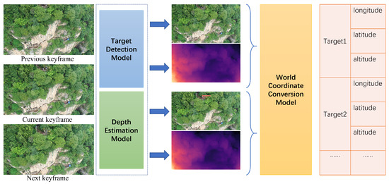
Figure 1.
The target detection model detects the current frame and outputs the pixel coordinates of targets. The depth estimation model in parallel with it uses the previous frame to perform depth estimation with the current frame and obtains the absolute depth based on the displacement information of UAV. Finally the coordinate conversion model combines the pixel coordinates with the depth information to obtain the global coordinate positioning of all targets.
Target positioning accuracy is influenced by various aspects such as UAV position accuracy, flight altitude, and speed. Since the remote sensing image and UAV flight information are transmitted separately, we mark the two kinds of information separately. The alignment of the two types of information is achieved in milliseconds by tagging and linear calculation. This reduces the impact of the UAV flight speed on the positioning error. Additionally, in the mission, the flight speed of the UAV should be proportional to the height relative to the scanned area. This is to ensure that the IOU of the area corresponding to the front and back frames at the same time interval remains within a more stable range. In order to take into account the flight safety and the clarity of the image, we generally position the flight height around 40 m and the flight speed is 8 m/s.
3.2. Depth Estimate
The main idea is to establish the function relationship between optical flow information and depth information by converting optical flow information into parallax information.
Considering that the rotation of the camera causes a significant change in the optical flow information, the optical flow information is corrected using the rotation information of the UAV before the calculation. Then by transforming the optical flow information through the camera coordinate system, the scaling factor is obtained as the relative depth of the camera displacement length. In the following, we will explain the method in several key steps.
3.2.1. Optical Flow Correct
The pixel coordinate transformation caused by camera rotation is independent of the depth information. The optical flow noise caused by rotation can be obtained by back-projecting the pixel coordinates to the camera coordinate system, then reprojecting them to the pixel coordinate system after the coordinate rotation transformation. By subtracting the optical flow noise from the result of the optical flow estimation model, we can obtain the optical flow information in the same directional view.
The inverse projection calculation requires the parameters of the camera. After calibrating the camera, we obtain the internal reference matrix, denoted as . This matrix represents the projection of the camera coordinate system with respect to the pixel coordinate system.
where denotes the pixel coordinates and is the spatial position in the current camera coordinate system corresponding to the pixel coordinates.
The inverse matrix of is denoted as . The formula for the inverse projection is expressed as:
denotes the corresponding point of the pixel point in the plane of m in the camera coordinate system.
The calculation also involves the rotational change of the spatial coordinate system. If the angles of rotation around the three axes are set to , , and , then the rotation matrices around each of the three axes are
The rotation can be decomposed into three steps. (1) The camera coordinate system rotates around the x-axis , so that the z-axis is horizontal. (2) Rotates around the y-axis , so that the projection of both z-axis on the horizontal plane is in the same direction. (3) Rotates around the x-axis again , so that the two coordinate systems are in the same direction of the three axes. and are the corresponding pitch angle of the two frames, while , represent the yaw angle of the camera. The rotation matrix is expressed by the equation as:
Combining the above formulas, the angle correction is calculated as follows:
represents the optical flow information estimated by the model for the two frames, and is what we need, after rotation correction.
3.2.2. Depth Computing
The main idea is to combine the optical flow, , with the displacement of the camera to construct similar triangles. The depth information of the current frame is derived by equiproportional calculation. We choose a plane in the 3D coordinate system to illustrate the construction of the triangle, as shown in Figure 2.
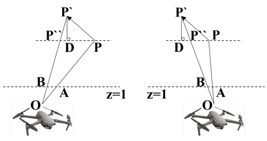
Figure 2.
Illustration of depth calculation for any pair of corresponding points.
To facilitate the calculation, we use inverse projection to transform the pixel coordinates so that all coordinate calculations can be placed under the same camera coordinate system. The point P is the real position of any point in the current frame to one, and is the position of point P in the previous frame relative to the camera. After point P make a parallel line parallel to and intersect the line where is at the point . Thus, we obtain a set of similar triangles, with . The absolute depth of point P, denoted as , is
The length of can be found by through the inverse projection. is perpendicular to with the vertical point D. is divided into two parts. is the projection of camera displacement in the direction of and is the correction to the previous value. Figure 2 shows two different positions of the points in relation to the camera, corresponding to the cases where the correction value is greater than zero and less than zero, respectively. The correction value is influenced by and , and is opposite in sign to the cosine of the angle between these two vectors.
The length of can be found by the Rt. Set the coordinates of point C as , which is the projection point of O on the plane . We achieve the solution for the length of by constructing the second pair of equivalence relations as follows:
Finally, combining the above equations, the absolute depth is solved by:
3.3. World Coordinate Calculation
The function of this method is to convert pixel coordinates to world coordinates. The main process is divided into two parts. First, converting pixel to camera coordinates, and then continuing the conversion to world coordinates through the both spatial coordinate system conversion relationship.
Record the longitude of the camera as L, the latitude as B, and the elevation as H. The Z-axis of camera coordinate system coincides with the camera optical axis, and the direction is outward, so it only needs to be positively rotated around the X-axis by a pitch angle, noted as p, and the Z-axis direction is vertical to the horizontal plane. Then, rotate B around the Y-axis, and finally rotate the Z-axis , the three axis direction and the geocentric coordinate system to maintain the same. Finally, the formula of rotation matrix is:
The origin of the camera coordinate system can be regarded as the position of the UAV, which is written as , and the center of the circle of the geocentric coordinate system is written as . Then is the geocentric coordinate of the UAV, which is written as . The conversion method through latitude, longitude and elevation is:
where the equatorial radius of the reference ellipsoid is noted as a and the polar radius of the reference ellipsoid is b.
Finally, the conversion process of the target pixel coordinates is summarized as:
4. Results
In this section, we will show the positioning effect of our method in practical applications. The experiments are divided into four parts: (1) optical flow model training, (2) depth calculation, and (3) target localization experiments in complex environments.
4.1. Models Training
4.1.1. Optical Flow Model
The purpose of introducing the optical flow estimation model is to find the correspondence between the pixel coordinates in two frames. We select the currently well-performing model, RAFT [33], and train it. It takes the optical flow estimation problem and estimates the motion of all pixels end-to-end using deep neural networks and achieves higher accuracy and robustness than other optical flow algorithms. It has strong generalization over many datasets, so we think it can also have good performance in remote sensing images. RAFT performs well in terms of number of parameters, inference time, which can meet the real-time requirements well. We reprojected remote sensing images of complex terrain based on depth information with random orientation camera positional changes to form the dataset used for network training. We show part of the dataset, as well as the test results in Figure 3.
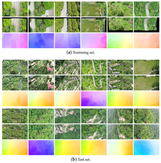
Figure 3.
Parts of dataset are shown. Each piece of data are divided into three parts, A (first row), B (second row), and flow (third row). Flow is the pixel motion relationship from A to B. In the training set, A is the original image and B is the reprojected image. In the test set, A is the previous frame image and B is the current frame image.
The whole dataset consists of 20 videos with a frame rate of 30 frames/s. The UAVs fly at 20–60 m and have a flight speed of 1 m/s. The scene contents of the videos mainly include forests, steep cliffs, mountains, etc. We obtained 7201 images by extracting key frames, and modeled the scene through SLAM method. The modeling results serve as the reference value source for depth information. The scene with point cloud is displayed in Figure 4. We amplified all images by performing multiple random direction reprojection operations on each one, and finally obtained a dataset containing 36,005 images. The training set and verification set are randomly allocated according to the ratio of 8:2.
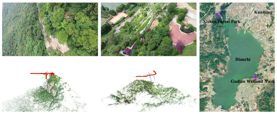
Figure 4.
Data set collection and experimental scenes. The scene on the left is Xishan Forest Park (N E) and on the right is Gudian Wetland Park (N E).
4.1.2. Target Detection Model
We trained each of the five models with different specifications and complexity of YOLOv5, in descending order of network complexity, YOLOv5n, YOLOv5s, YOLOv5m, YOLOv5l, and YOLOv5x. The datasets used for training and testing are from the same source as the datasets used for training the optical flow model. To enlarge the dataset size, we used data enhancement methods including rotation, scaling, and single-shoulder transformation. The dataset contains 3080 images and 45,096 target labels. The ratio of training set to validation set is about 8:2. The trends of precision and recall in training are shown in Figure 5. The performance effect of each model is shown in the Table 1. The represents the time required to process an image when the target detection model is invoked alone. The comparison results show that YOLOv5 performs the best in terms of the combined evaluation criteria of accuracy and recall. The YOLOv5x model is the preferred choice for the experiments provided that the real-time requirements are met. Considering the need to access two neural network models at the same time and to ensure the real-time performance of the operation, we used YOLOv5l for the subsequent experiments.
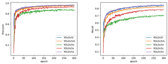
Figure 5.
The variation trend of precision (left) and recall (right) during training.

Table 1.
Performance of different models on the RTX 2070 Super.
4.2. Depth Calculation
In the experiment, we used the pictures collected in the places shown in Figure 4 that did not appear in the training set to form the test set. The test set contains 604 images, which are composed of three video key frames. Considering that our method requires two adjacent frames for computation, we compared the results of except the first key frame of each video.
We evaluated the effectiveness of our method by comparing it with the reference depth theywere born using the SLAM method. We likewise compare with three other methods, Monodepth2 [34], Madhuanand et al. [24], and CADepth [35]. Monodepth2 [34] uses a joint training approach to train both PoseNet and DepthNet using consecutive image sequences for self-supervised training. Madhuanand et al. [24] proposes for the first time to train a depth estimation model using tilted drone videos. All these models are trained under the same environment, dataset, and resolution as our method to make them comparable.
To evaluate the performance, we compared the Madhuanand et al. [24] according to a series of metrics. These include Absolute Relative difference (Abs Rel), given in Equation (13), used to calculate the average difference between the reference and corresponding pixel position of the method’s predicted depth, Squared Relative difference (Sq Rel) as given in Equation (14) which is used to represent the squared difference between reference and method predicted depth, Root Mean Square Error (RMSE), given in Equation (15), accuracy as given in Equation (16).
where is the reference depth of each pixel at the position and is the method predicted depth at the position. The accuracy of Equation (16) is the percentage of pixels within a certain threshold . Based on the standard benchmarks of KITTI quantitative evaluation, the thresholds are chosen as , , and . The predicted depths of our method with these depth estimation models are visualized in Figure 6. The quantitative evaluation results are shown in Table 2. In steep and rugged scenes, our method has higher accuracy. It is also obvious from the depth information visualization images that the depth distribution predicted by our method is more consistent with the real depth distribution and is not limited by the inherent depth distribution trend at any angle, in any terrain.
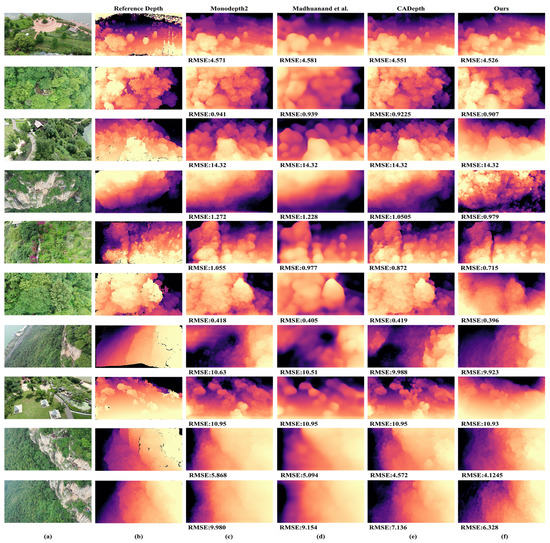
Figure 6.
Qualitative comparison between (b) reference depths from SLAM, (c) Monodepth2 [34], (d) Madhuanand et al. [24], (e) CADepth [35], (f) ours. The test image is given in (a).

Table 2.
Comparison of assessment results.
Areas with larger depth values are colored blue-purple, and smaller ones are yellow. Our method has clearer edges in a variety of scenes including cliffs, woods, slopes, etc. Additionally, in a variety of depth distribution trends, our method can better and more accurately reflect the changes in depth. However, in the edge region, our method sometimes has errors, especially when the true depth value of the image edge varies widely. Since there are no moving objects involved in the test set, the effect of depth prediction for moving objects is not reflected in the test images. We also performed a quantitative evaluation to compare the effects between several methods more accurately.
The quantitative metrics between the methods are shown in Table 2. The data in the table are the evaluation metrics calculated by calculating the ratio of the reference depth to the mean value of the predicted depth of each method, after scaling the predicted depth. From the table, we can observe that our method achieves the best results for all three evaluation metrics, Abs Rel, Sq Rel, and RMSE. At a threshold of 1.05, the accuracy of our method is second only to CADepth and obtains the best results with the same effect as CADepth at a threshold of 1.25.
4.3. Positioning in Complex Scenes
To demonstrate the effectiveness and accuracy of the method in complex scenes, we designed several field positioning experiments. Experimenters were dispersed into scenes as positioning targets. These scenes included hills, woods, cliffs, etc. The experiments were conducted in the Xishan Forest Park (N E) and the Gudian Wetland Park (N E). The target localization calculation was partially run on a laptop with an i7-10875H CPU, RTX 2070 SUPER GPU and 16GB RAM. The computation speed can reach more than 25 frames per second, which meets the real-time requirement. Finally, the calculated points are displayed in the form of coordinates in Figure 7. The error results of target localization are shown in Table 3.
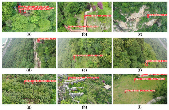
Figure 7.
Target positioning result display. The positioning results shown in each image are consistent with the Positioning Lng, Lat column in Table 3. The scene in (a–f) is in the Xishan Forest Park, which has steep terrain and contains complex environments such as mountain roads and cliffs. The scene in (g–i) is in Gudian Wetland Park, with selected scenes of woods, meadows, etc.

Table 3.
Target positioning result.
The error distance of localization is derived by calculating the spatial distance between the true and predicted coordinates. As can be seen from the settlement results in the table, of positioning accuracy errors remain within 5 m in complex scenarios. The overly steep environment is still generally lower than the positioning accuracy in other environments. However, the error can still be guaranteed to be within 8 m. Overall, this method can meet the positioning requirements in complex scenes.
We cite different depth estimation methods involved in positioning for comparing the effect of depth estimation methods on positioning errors. Since the exact distance from the camera to a plane is not available in a complex environment, the scale factor of the depth map cannot be calculated by predicting the camera height during the experiment. We designed a computational method for the calculation of scale factor. This method derives the scale factor corresponding to two depth maps by the different representations of two depth maps with different UAV positions at the same spatial point. The formula is as follows:
where is a set of determined corresponding points, is the relative depth information corresponding to this pair of points, and is the rotation matrix of the UAV. The equation can be solved for three unknowns. is the scale factor corresponding to the two depth maps. b represents the error distance, and the scaling factor is more accurate only when the value of B is smaller. In the experiment, the absolute value of b is limited to less than 0.2, which represents the selected corresponding point at a distance less than 0.2 m in space.
The analysis of the positioning errors after plugging different depth estimation models into the target positioning method is shown in Table 4. We calculated the minimum, maximum, and average values of the errors, and counted the proportion of samples with errors within 3 m, 5 m, and 8 m of the total samples, respectively. From the table, we can see that the target localization results using our depth estimation method have smaller errors overall and more stable results.

Table 4.
Target positioning result with different depth estimate method.
5. Discussion
In this paper, a new method is proposed for estimating the depth information of UAV videos in complex scenes. This method is used to improve the accuracy of target localization in complex scenes. The method we propose requires a progressive depth calculation based on the pixel coordinate relationship between frames based on the motion information of the UAV. The pixel motion used in the computation is predicted by the trained optical flow estimation model. Although supervised training is performed, the supervised signal can be obtained by reprojection calculation, which is less difficult to obtain and more accurate. Moreover, the trained model is not limited by the original terrain type because it is detached from the original scene of the terrain, and can be used for a variety of multi-angle complex scenes.
In terms of target positioning, the computational process that introduces depth estimation is detached from the dependence on elevation information and assumed planes, which allows for much higher positioning accuracy in complex terrain, especially in scenes with large elevation changes. The calculation of depth information is related to the pixel motion distance. The smaller the pixel motion distance is, the larger the depth estimation error is. When the displacement of the UAV is parallel to the imaging plane of the camera, the pixel motion distance corresponding to the same spatial point reaches the maximum and the depth estimation is the most accurate.
In our future work, we will further explore the depth estimation methods for remote sensing videos in complex scenes, improve the depth estimation accuracy for reflective and dynamic objects, and further improve the accuracy of target localization methods.
Author Contributions
Conceptualization, L.X.; methodology, L.X.; software, L.X. and K.Y.; validation, L.X. and K.Y.; formal analysis, L.X.; investigation, L.X.; resources, L.X.; data curation, L.X.; writing—original draft preparation, L.X.; writing—review and editing, L.X. and Y.Y.; visualization, L.X.; supervision, Y.Y.; project administration, Y.Y.; funding acquisition, Y.Y. and L.X. All authors have read and agreed to the published version of the manuscript.
Funding
This research was funded by Graduate Research and Innovation Fund of Yunnan Normal University (YJSJJ22-B112).
Data Availability Statement
The data presented in this study are available on request from the corresponding author. The data are not publicly available due to privacy issues such as portraits of people other than the experimenters involved in the data collection process.
Conflicts of Interest
The authors declare no conflict of interest. The funders had no role in the design of the study; in the collection, analyses, or interpretation of data; in the writing of the manuscript, or in the decision to publish the results.
Abbreviations
The following abbreviations are used in this manuscript:
| UAV | Unmanned Aerial Vehicle |
| SLAM | Simultaneous Localization and Mapping |
References
- Chen, J.; Chen, S.; Chen, X.; Yang, Y.; Rao, Y. StateNet: Deep State Learning for Robust Feature Matching of Remote Sensing Images. IEEE Trans. Neural Netw. Learn. Syst. 2021, 1–15. [Google Scholar] [CrossRef] [PubMed]
- Chen, J.; Chen, S.; Chen, X.; Yang, Y.; Xing, L.; Fan, X.; Rao, Y. LSV-ANet: Deep Learning on Local Structure Visualization for Feature Matching. IEEE Trans. Geosci. Remote Sens. 2021, 60, 4700818. [Google Scholar] [CrossRef]
- Chen, J.; Chen, S.; Liu, Y.; Chen, X.; Yang, Y.; Zhang, Y. Robust Local Structure Visualization for Remote Sensing Image Registration. IEEE J. Sel. Top. Appl. Earth Obs. Remote Sens. 2021, 14, 1895–1908. [Google Scholar] [CrossRef]
- Chen, J.; Fan, X.; Chen, S.; Yang, Y.; Bai, H. Robust Feature Matching via Hierarchical Local Structure Visualization. IEEE Geosci. Remote Sens. Lett. 2021, 19, 8018205. [Google Scholar] [CrossRef]
- Chen, S.; Chen, J.; Xiong, Z.; Xing, L.; Yang, Y.; Xiao, F.; Yan, K.; Li, H. Learning Relaxed Neighborhood Consistency for Feature Matching. IEEE Trans. Geosci. Remote Sens. 2021, 60, 4702913. [Google Scholar] [CrossRef]
- Liu, Y.; Gong, X.; Chen, J.; Chen, S.; Yang, Y. Rotation-Invariant Siamese Network for Low-Altitude Remote-Sensing Image Registration. IEEE J. Sel. Top. Appl. Earth Obs. Remote Sens. 2020, 13, 5746–5758. [Google Scholar] [CrossRef]
- Ma, J.; Tang, L.; Fan, F.; Huang, J.; Mei, X.; Ma, Y. SwinFusion: Cross-domain Long-range Learning for General Image Fusion via Swin Transformer. IEEE/CAA J. Autom. Sin. 2022, 9, 1200–1217. [Google Scholar] [CrossRef]
- Tang, L.; Deng, Y.; Ma, Y.; Huang, J.; Ma, J. SuperFusion: A Versatile Image Registration and Fusion Network with Semantic Awareness. IEEE/CAA J. Autom. Sin. 2022, 9, 2121–2137. [Google Scholar] [CrossRef]
- Manfreda, S.; McCabe, M.F.; Miller, P.E.; Lucas, R.; Pajuelo Madrigal, V.; Mallinis, G.; Ben Dor, E.; Helman, D.; Estes, L.; Ciraolo, G.; et al. On the Use of Unmanned Aerial Systems for Environmental Monitoring. Remote Sens. 2018, 10, 641. [Google Scholar] [CrossRef]
- Ventura, D.; Bonifazi, A.; Gravina, M.F.; Belluscio, A.; Ardizzone, G. Mapping and Classification of Ecologically Sensitive Marine Habitats Using Unmanned Aerial Vehicle (UAV) Imagery and Object-Based Image Analysis (OBIA). Remote Sens. 2018, 10, 1331. [Google Scholar] [CrossRef]
- Xing, L.; Fan, X.; Dong, Y.; Xiong, Z.; Xing, L.; Yang, Y.; Bai, H.; Zhou, C. Multi-UAV cooperative system for search and rescue based on YOLOv5. Int. J. Disaster Risk Reduct. 2022, 76, 102972. [Google Scholar] [CrossRef]
- Alotaibi, E.T.; Alqefari, S.S.; Koubaa, A. LSAR: Multi-UAV Collaboration for Search and Rescue Missions. IEEE Access 2019, 7, 55817–55832. [Google Scholar] [CrossRef]
- Rusnak, M.; Sladek, J.; Kidova, A.; Lehotsky, M. Template for high-resolution river landscape mapping using UAV technology. Measurement 2017, 115, 139–151. [Google Scholar] [CrossRef]
- Langhammer, J.; Vacková, T. Detection and Mapping of the Geomorphic Effects of Flooding Using UAV Photogrammetry. Pure Appl. Geophys. 2018, 175, 3223–3245. [Google Scholar] [CrossRef]
- James, M.R.; Chandler, J.H.; Eltner, A.; Fraser, C.; Miller, P.E.; Mills, J.P.; Noble, T.; Robson, S.; Lane, S.N. Guidelines on the use of structure-from-motion photogrammetry in geomorphic research. Earth Surf. Process. Landf. 2019, 44, 2081–2084. [Google Scholar] [CrossRef]
- Yan, K.; Li, Q.; Li, H.; Wang, H.; Fang, Y.; Xing, L.; Yang, Y.; Bai, H.; Zhou, C. Deep learning-based substation remote construction management and AI automatic violation detection system. IET Gener. Transm. Distrib. 2022, 16, 1714–1726. [Google Scholar] [CrossRef]
- Dyson, J.; Mancini, A.; Frontoni, E.; Zingaretti, P. Deep Learning for Soil and Crop Segmentation from Remotely Sensed Data. Remote Sens. 2019, 11, 1859. [Google Scholar] [CrossRef]
- Dan, P.; Stoican, F.; Stamatescu, G.; Ichim, L.; Dragana, C. Advanced UAV–WSN System for Intelligent Monitoring in Precision Agriculture. Sensors 2020, 20, 817. [Google Scholar] [CrossRef]
- Hua, J.; Cheng, M. Binocular Visual Tracking Model Incorporating Inertial Prior Data. In Proceedings of the 2020 IEEE 4th Information Technology, Networking, Electronic and Automation Control Conference (ITNEC), Chongqing, China, 12–14 June 2020; Volume 1, pp. 1861–1865. [Google Scholar] [CrossRef]
- Xu, S.; Dong, Y.; Wang, H.; Wang, S.; Zhang, Y.; He, B. Bifocal-Binocular Visual SLAM System for Repetitive Large-Scale Environments. IEEE Trans. Instrum. Meas. 2022, 71, 1–15. [Google Scholar] [CrossRef]
- dong Guo, X.; bo Wang, Z.; Zhu, W.; He, G.; bin Deng, H.; xia Lv, C.; hai Zhang, Z. Research on DSO vision positioning technology based on binocular stereo panoramic vision system. Def. Technol. 2022, 18, 593–603. [Google Scholar] [CrossRef]
- Ma, Y.; Li, Q.; Chu, L.; Zhou, Y.; Xu, C. Real-Time Detection and Spatial Localization of Insulators for UAV Inspection Based on Binocular Stereo Vision. Remote Sens. 2021, 13, 230. [Google Scholar] [CrossRef]
- Sun, J.; Li, B.; Jiang, Y.; Wen, C. A Camera-Based Target Detection and Positioning UAV System for Search and Rescue (SAR) Purposes. Sensors 2016, 16, 1778. [Google Scholar] [CrossRef]
- Madhuanand, L.; Nex, F.; Yang, M.Y. Self-supervised monocular depth estimation from oblique UAV videos. ISPRS J. Photogram. Remote Sens. 2021, 176, 1–14. [Google Scholar] [CrossRef]
- Nagata, C.; Torii, A.; Doki, K.; Ueda, A. A Position Measurement System for a Small Autonomous Mobile Robot. In Proceedings of the 2007 International Symposium on Micro-NanoMechatronics and Human Science, Nagoya, Japan, 11–14 November 2007; pp. 50–55. [Google Scholar] [CrossRef]
- Porter, R.; Shirinzadeh, B.; Choi, M.H.; Bhagat, U. Laser interferometry-based tracking of multirotor helicopters. In Proceedings of the 2015 IEEE International Conference on Advanced Intelligent Mechatronics (AIM), Busan, Republic of Korea, 7–11 July 2015; pp. 1559–1564. [Google Scholar] [CrossRef]
- Mo, Y.; Zou, X.; Situ, W.; Luo, S. Target accurate positioning based on the point cloud created by stereo vision. In Proceedings of the 2016 23rd International Conference on Mechatronics and Machine Vision in Practice (M2VIP), Nanjing, China, 28–30 November 2016; pp. 1–5. [Google Scholar] [CrossRef]
- Liu, Y.; Hu, L.; Xiao, B.; Wu, X.Y.; Chen, Y.; Ye, D.; Hou, W.S.; Zheng, X. Design of Visual Gaze Target Locating Device Based on Depth Camera. In Proceedings of the 2019 IEEE International Conference on Computational Intelligence and Virtual Environments for Measurement Systems and Applications (CIVEMSA), Tianjin, China, 14–16 June 2019; pp. 1–5. [Google Scholar] [CrossRef]
- Wang, R.; Pizer, S.M.; Frahm, J.M. Recurrent Neural Network for (Un-)Supervised Learning of Monocular Video Visual Odometry and Depth. In Proceedings of the 2019 IEEE/CVF Conference on Computer Vision and Pattern Recognition (CVPR), Long Beach, CA, USA, 15–20 June 2019; pp. 5550–5559. [Google Scholar] [CrossRef]
- Ling, C.; Zhang, X.; Chen, H. Unsupervised Monocular Depth Estimation Using Attention and Multi-Warp Reconstruction. IEEE Trans. Multimed. 2022, 24, 2938–2949. [Google Scholar] [CrossRef]
- Takamine, M.; Endo, S. Monocular Depth Estimation with a Multi-task and Multiple-input Architecture Using Depth Gradient. In Proceedings of the 2020 Joint 11th International Conference on Soft Computing and Intelligent Systems and 21st International Symposium on Advanced Intelligent Systems (SCIS-ISIS), Hachijo Island, Japan, 5–8 December 2020; pp. 1–6. [Google Scholar] [CrossRef]
- Watson, J.; Mac Aodha, O.; Prisacariu, V.; Brostow, G.; Firman, M. The Temporal Opportunist: Self-Supervised Multi-Frame Monocular Depth. In Proceedings of the 2021 IEEE/CVF Conference on Computer Vision and Pattern Recognition (CVPR), Nashville, TN, USA, 19–25 June 2021; pp. 1164–1174. [Google Scholar] [CrossRef]
- Teed, Z.; Deng, J. RAFT: Recurrent All-Pairs Field Transforms for Optical Flow. arXiv 2020, arXiv:2003.12039. [Google Scholar]
- Godard, C.; Aodha, O.M.; Firman, M.; Brostow, G. Digging Into Self-Supervised Monocular Depth Estimation. In Proceedings of the 2019 IEEE/CVF International Conference on Computer Vision (ICCV), Seoul, South Korea, 27 October–2 November 2019; pp. 3827–3837. [Google Scholar] [CrossRef]
- Yan, J.; Zhao, H.; Bu, P.; Jin, Y. Channel-Wise Attention-Based Network for Self-Supervised Monocular Depth Estimation. arXiv 2021, arXiv:2112.13047. [Google Scholar]
Disclaimer/Publisher’s Note: The statements, opinions and data contained in all publications are solely those of the individual author(s) and contributor(s) and not of MDPI and/or the editor(s). MDPI and/or the editor(s) disclaim responsibility for any injury to people or property resulting from any ideas, methods, instructions or products referred to in the content. |
© 2023 by the authors. Licensee MDPI, Basel, Switzerland. This article is an open access article distributed under the terms and conditions of the Creative Commons Attribution (CC BY) license (https://creativecommons.org/licenses/by/4.0/).