Article

Analysis of Temperature Semi-Annual Oscillations (SAO) in the Middle Atmosphere

1
School of Geography and Information Engineering, China University of Geosciences, Wuhan 430074, China
2
Hubei Subsurface Multi-Scale Imaging Key Laboratory, Institute of Geophysics and Geomatics, China University of Geosciences, Wuhan 430074, China
3
Department of Atmospheric Science, China University of Geosciences, Wuhan 430074, China
4
Centre for Severe Weather and Climate and Hydro-Geological Hazards, Wuhan 430074, China
5
Research Centre for Complex Air Pollution of Hubei Province, Wuhan 430074, China
*
Author to whom correspondence should be addressed.
Remote Sens. 2023, 15(3), 857; https://doi.org/10.3390/rs15030857
Submission received: 5 November 2022 / Revised: 18 January 2023 / Accepted: 31 January 2023 / Published: 3 February 2023

Abstract

:
The middle atmosphere plays an important role in the research of various dynamical and energy processes. Microwave Limb Sounder (MLS), reanalyses and model simulations with NCAR’s Whole Atmosphere Community Climate Model (WACCM) data in the range between 100 and 0.1 hPa from 2005 to 2020 have been analyzed with a focus on the temperature semi-annual oscillations (SAO). Significant SAO of temperature is prominent in the tropical region (20 ° S–20 ° N) around 1–3 hPa, which is consistent with previous studies. We also found significant SAO in the northern hemisphere (NH) high latitudes between 8 and 0.3 hPa and southern hemisphere (SH) high latitudes between 0.5 and 0.1 hPa, which has been of less concern in previous studies. The thermal budget based on MERRA2 and simulations is used to explain the mechanism of SAO in the middle atmosphere. In the tropics, the two temperature peaks are mainly determined by radiative processes. In the NH high latitudes of the stratosphere, the temperature peak in January is mainly related to dynamical processes, while the temperature peak in July is determined by a combination of dynamical and radiative processes. In the NH high latitudes of the lower mesosphere, the first peak in June is primarily associated with dynamical and radiative processes, while the second peak in December is primarily associated with the dynamical processes. In the SH high latitudes of the lower mesosphere, the first temperature peak in July is mainly due to dynamical processes while the second temperature peak in December is mainly due to radiative processes. Various features are present in the SH and NH high latitude SAO in the lower mesosphere. Furthermore, we performed model simulations with and without SAO in sea surface temperatures (SST-SAO) to study the connection between SST and temperature SAO. WACCM6 results indicate that the SAO in the middle atmosphere is partially affected by the existence of an SST-SAO. By removing SAO in SST, the PSD magnitude of the SAO decreases in the tropical region and increases in the polar region. The amplitudes of total heating rates are also modified. The WACCM experiment confirms the relationship between SST-SAO and temperature SAO in the middle atmosphere.

1. Introduction

Various oscillations from diurnal to interannual time scales in temperature and wind have been extensively studied in the middle atmosphere [1,2,3]. Among them, the semi-annual oscillations (SAO) of the wind and temperature field is one of the most interesting components. The SAO in the middle atmosphere is notable mainly in two regions, with one near the stratopause (∼1 hPa) and the other around the mesopause (∼0.01 hPa). A dominated SAO in temperature and wind fields in the equatorial region was first documented in the middle atmosphere in the 1960s [4,5,6]. The SAO in the stratosphere is related to the twice-yearly passage of the Sun across the equator and the strong absorption of solar ultraviolet radiation by ozone. As previously found [7], the stratospheric SAO in equatorial latitudes might be additionally associated with the winter circulation in the troposphere. Later research showed that the tropical stratospheric SAO was driven by wave–mean flow interactions [8,9]. Some studies [7,10,11] also indicated that the stratospheric temperature SAO exists in polar regions, but with a smaller amplitude compared to the annual cycle. The stronger SAO at the North Pole relative to the South Pole is due to polar stratospheric warming [10].
The SAO in the mesosphere is out of phase with the stratospheric SAO [12,13]. Many studies [14,15,16] have suggested that gravity and Kelvin waves, which are selectively transmitted by stratospheric SAO, were responsible for the equatorial SAO in the mesosphere. However, the research concerning the SAO in the mesosphere is still inadequate, especially for high latitudes because there are limited observations and there are still large uncertainties in the explanation of the SAO in the mesosphere. Most of radiosonde stations have data up to 10 hPa in the middle stratosphere. Lidar and sounding rocket measurements have only limited spatial and temporal coverage. As a consequence, model simulations are commonly used to study the mechanism of the SAO in the mesosphere [17,18]. However, model simulations have difficulties in simulating a realistic SAO in the middle atmosphere by, e.g., a lack of eastward forcing by waves [19]. The launch of the Microwave Limb Sounder (MLS) in the year 2004 makes it possible to assess the SAO in the mesosphere especially in high latitudes. Recent studies [20,21,22] show that a new set of observations is helpful for updating the observed temperature variability in the middle atmosphere.
The SPARC Reanalysis Intercomparison Project (S-RIP) compares temperature and wind in the middle atmosphere of all reanalyses to better understand the differences among different products and their underlying causes, to provide guidance to users and to establish collaborative links between the SPARC community and the reanalysis centers [23]. According to SPARC S-RIP reports [23], tropical SAO showed large differences by detailed comparison among reanalyses (CFSR, MERRA, ERA-Interim, JRA-55 and MERRA2) and one of the future evaluations is SAO variability. However, the comparison is between the surface and 10 hPa. In our study, the global spatio-temporal variation of the temperature SAO in the middle atmosphere is investigated with the latest data sets, i.e., the MLS satellite measurements and the latest ERA5 and MERRA2 reanalysis data. With the development of models and data assimilation techniques, the new generation of reanalyses has improved their ability to better represent the SAO in the middle atmosphere. In particular, the differences between the newest ERA5 and MERRA2 in the representation of SAO in the upper stratosphere and lower mesosphere would be interesting to both the SPARC community and the reanalysis centers.
In an earlier study [24], we studied the SAO in the upper troposphere and lower stratosphere (UTLS) based on GNSS RO, ERA5, MERRA2 and WACCM6. The result shows that the SAO in the UTLS is related to moisture and dynamical heating and also partly affected by the SST-SAO. However, the results are limited in the UTLS region up to 10 hPa. The SAO in temperature and zonal wind not only exists in the UTLS and at the surface, but is also noticed in the middle atmosphere. For instance, the predictability of the lower atmosphere can be improved by the middle atmosphere [25,26,27]. The goal of this paper is to show some new features and to give a comprehensive survey of the SAO in the middle atmosphere and also to try to give some explanation of the SAO formation through the thermal budget analysis. We also try to establish the connection between the SST-SAO and the SAO in the middle atmosphere. Simulation is a powerful tool to realize these purposes. Therefore, we also include WACCM6 to study the temperature SAO in the middle atmosphere due to its significant new capabilities (e.g., better representation of the chemistry, an internally generated QBO and improved climatology of sudden stratospheric warming) in the middle and upper atmosphere. In our case, we use the WACCM6 and MERRA2 thermal energy budget to reveal the mechanism of the SAO in the middle atmosphere. In addition, WACCM6 can be run coupled to an ocean [28]. With the help of WACCM6, we could explore the link between SST-SAO and the SAO in the middle atmosphere. We document the responses of temperature SAO throughout the upper stratosphere and lower mesosphere in a comprehensive whole atmosphere global model with different prescribed SST. Such a model setup can capture well the temperature variations in the middle atmosphere in responding to removed SAO in SSTs. It is of interest to quantify the magnitude temperature under different prescribed SST. Our study explores the feature of SAO in the middle atmosphere with the thermal energy budget and its possible connection with SST-SAO.
The organization of the paper is as follows: The used data sets and analysis methods are introduced in Section 2. Section 3 gives the results and discussion. In Section 3.1 and Section 3.2, a spatial and temporal variation of the SAO in the middle atmosphere is described in detail based on the spectrum analysis. In Section 3.3, we further analyze the thermal energy budget of the simulation and MERRA2 for the mechanism to drive the SAO. In Section 3.4, the relationship between the SAO in the middle atmosphere and SST-SAO is checked based on the model simulations and wavelet analysis. Section 4 summarizes and concludes the paper.

2. Data and Methods

2.1. MLS Data

The Aura MLS observations, which include atmospheric observations (e.g., temperature and ozone) from the upper troposphere to the mesosphere, started in July 2004 [29,30]. Aura orbit enables MLS measurements with a latitude coverage of 82 ° S to 82 ° N [31]. The MLS temperature data have been validated with many different instruments and analyses, and show good quality [32,33]. The MLS data used here are the monthly binned product version 5.1 for temperature derived from radiances measured by the 188 and 240 GHz radiometers at fixed pressure levels. They have a horizontal resolution of 4 ° × 5 ° (latitude × longitude) and can be downloaded from https://search.earthdata.nasa.gov/search?q=ML3MBT_005.thml, accessed on 27 August 2022. The vertical range from 261 to 0.001 hPa is recommended for use and 31 pressure levels from 100 to 0.1 hPa with a vertical resolution between 3 and 6 km are used in this study. In addition, the MLS ozone retrievals v5.1 (https://disc.gsfc.nasa.gov/datacollection/ML3MBO3_005.html, accessed on 27 August 2022) in the same region are used as assistant data for the analysis. More information about MLS products can be found in the study [34].

2.2. Reanalysis Data

We also analyzed the monthly zonal mean temperature from 2005 to 2020 in the range of 100 to 0.1 hPa in two sets of global reanalyses, i.e., ERA5 [35] and MERRA2 [36]. ERA5, which are released by the European Centre for Medium Range Weather Forecasts (ECWMF) in 2018, is used in this study. ERA5 with the model levels and a horizontal resolution of 1 ° are downloaded from Climate Data Store (CDS) [37]. In addition to the temperature product, MERRA2 also includes energy budget parameters. We used monthly mean heating rates and temperature products of MERRA2 [38,39]. Compared with ERA5, MERRA2 assimilates temperature data from Aura MLS above 5 hPa [40], which constrains the MERRA2 temperature even in the mesosphere. The MERRA2 with spatial resolution 1.25 ° are downloaded by the Global Modeling and Assimilation Office (GMAO). In total, 18 pressure levels from 100 to 0.1 hPa are extracted from MERRA2 data. Compared to MERRA2, ERA5 has a higher vertical resolution (56 selected pressure levels in the range of 100 to 0.1 hPa).

2.3. WACCM

WACCM6 is a general circulation model of the whole atmosphere from the surface to 140 km in the Community Earth System Model (CESM), which is provided by the National Center for Atmospheric Research (NCAR) [27]. CESM2 is used in the configuration. WACCM6 improves the atmospheric chemistry, stratospheric variability (a self-generated quasi-biennial oscillation and improved climatology of sudden stratospheric warming) and volcanic aerosols. It allows studying the propagation of signals of various phenomena and possible processes that connect two far distant regions. We use the atmosphere-only mode with prescribed SSTs at 70 standard vertical levels. We chose 29 levels from 100 to 0.1 hPa with a horizontal resolution 1.9 ° latitude by 2.5 ° longitude to show in this study. We first employ a hindcast simulation (hereafter termed the control run), with prescribed Hadley Centre SSTs [41] and forcing by historically observed values (e.g., greenhouse gases, ozone-depleting substances) over the period from 1995 to 2020 [28]. The first 10 years (1995–2004) are not analyzed to provide a spin-up. The solar and geomagnetic forcing used in the model is described in the study [42]. WACCM6 runs with the interactive ocean are helpful to check the relationship between the temperature SAO in the middle atmosphere and SST-SAO. We employ two additional simulations (rmSAO and rmSAO-TP) with the same climate forcing but different prescribed SSTs [24]. The SSTs are adjusted to remove the SAO (signals between 5 and 7 months) globally (rmSAO run) and in the tropics (rmSAO-TP run) by a band-pass filter based on the Butterworth method [43], respectively.

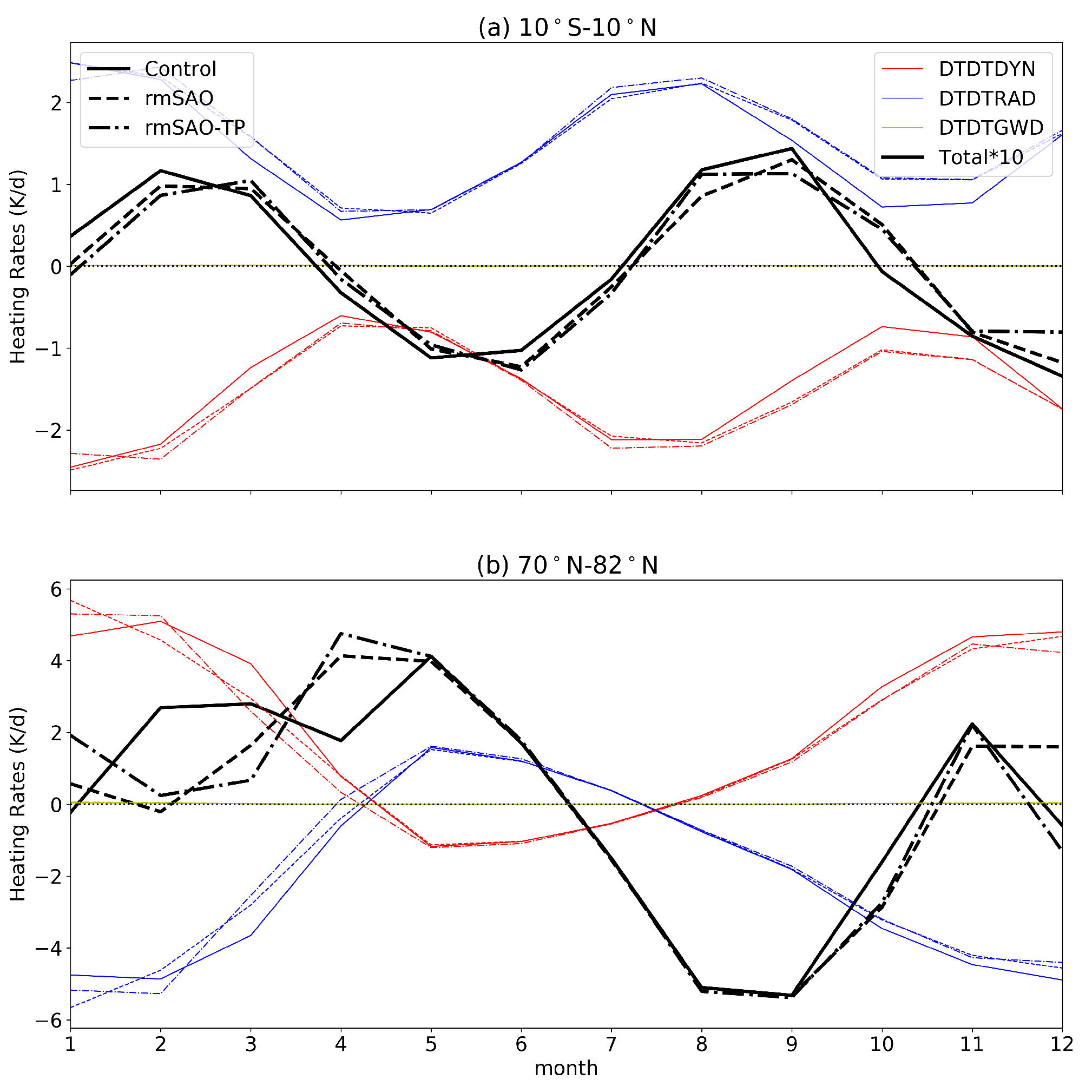
2.4. Thermal Energy Budget

The thermal budget of the MERRA2 and model simulations are used to analyze the temperature SAO. WACCM6 could provide an atmosphere energy budget and cloud radiative effects up to their top. The temperature tendencies related to dynamics, radiation, moisture and gravity wave drag processes are provided in the WACCM6 [27]. The radiation term is the sum of long-wave and short-wave terms in the simulation. Here we use the dynamics, radiation and gravity wave drag terms in this study. The formulation for the thermodynamic balance is [44,45]:
T t ¯ = v ¯ * T y ¯ w ¯ * S e z H [ e z H ( v t ¯ T y ¯ S + w T ¯ ) ] z + Q ¯
v ¯ * = v ¯ ρ 0 1 [ ρ 0 v Θ ¯ / Θ ¯ z ] z
w ¯ * = w ¯ + ( a c o s ϕ ) 1 [ c o s ϕ v Θ ¯ / Θ ¯ z ] ϕ
where ρ 0 is the atmosphere density, Θ is potential temperature and ϕ is latitude. S = H N 2 R with R = 287 m 2 s 2 K 1 , H = 7 km. N 2 is the Brunt-V a ¨ is a ¨ l a ¨ frequency. The overbars of the equation denote zonal averages, the prime numbers denote deviations from it and the indices denote partial derivatives. The components of the residual circulation v ¯ * and w ¯ * are calculated via Equations (2) and (3). w ¯ (converted from the vertical pressure velocity) is the zonal mean vertical velocity. The dynamical heating includes the first three terms on the right side of Equation (1), which denote heating by the meridional component of the residual circulation, the heating/cooling by downwelling/upwelling and heating related to eddys, respectively. Q is the radiative heating.
MERRA2 also provides detailed temperature tendencies related to dynamics (DTDTDYN), radiation (DTDTRAD), moisture (DTDTMST), friction (DTDTFRI), gravity wave drag (DTDTGWD), near-surface turbulence (DTDTTRB) and analysis tendencies (DTDTANA), which is a residual to keep a balance of the thermal budget during the data assimilation. The DTDTANA can be considered as the negative of model physical process errors and the DTDTDYN includes advection of resolved-scale gradients by resolved-scale flows, pressure gradient and Coriolis [46]. More details for the thermal energy budget can be found in previous studies [24,46].

2.5. Time Series Analysis

Spectrum analysis and wavelet analysis were performed to study the spatio-temporal variation of the SAO. A periodogram is used to detect periodic signatures in the temperature data. The periodogram, which is the Fourier transform of the biased estimate of the autocorrelation sequence, is used to estimate the power spectral density (PSD) [47,48]. A Fisher’s g-statistic is used to calculate the statistical significance for a false discovery rate (FDR) level of 0.05, which distinguishes periodical processes from purely random processes. Fisher’s g-statistic uses the ratio of the largest periodogram value to the sum of all periodogram values over half of the frequency interval [49]. To study the statistical relationship between temperature SAO and SST-SAO, the 1D wavelet Morlet transform is firstly used to extract SAO signals (5–7 months) [50,51]. For the correlation analysis, we use the Pearson correlation coefficient and the statistical significance with a Student’s t-test.

3. Results and Discussion

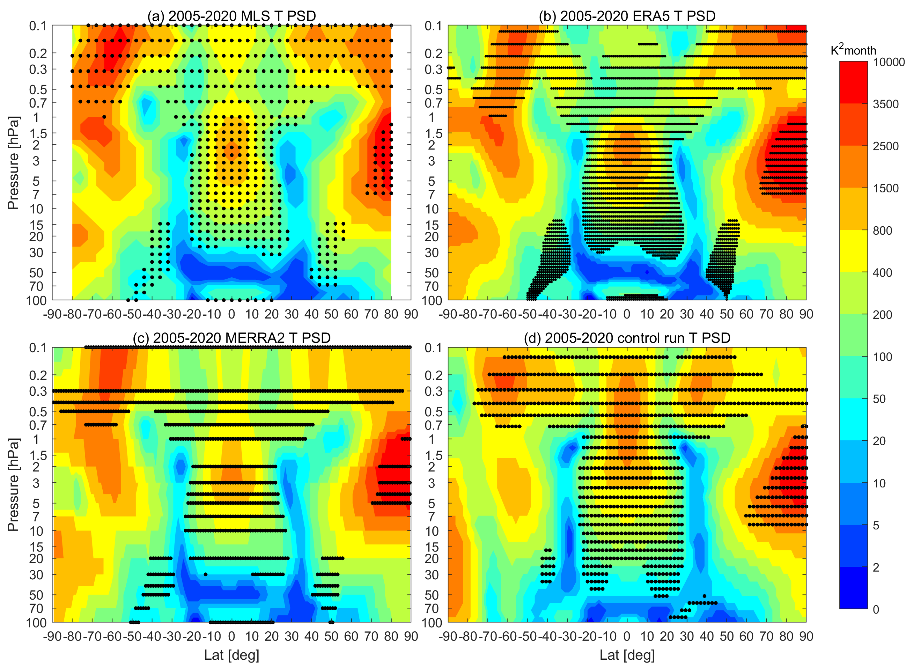
3.1. Spatial Analysis of the SAO

According to the periodogram PSD values of the zonal mean temperature SAO from 2005 to 2020 (Figure 1a–d), the semi-annual cycle is significant in tropical regions (20 ° S–20 ° N) from 30 to 0.1 hPa and also in mid and high latitudes from 0.5 to 0.1 hPa in MLS, ERA5, MERRA2 and simulation data. The model simulation and reanalyses show good agreement with MLS for the general pattern of the SAO PSD in Figure 1. Most data sets show a peak of the PSD magnitude around 1–3 hPa near the equator, around 0.3–0.1 hPa in high latitudes and the North Pole between 8 and 1 hPa. The observed maximum SAO over the equator in the stratosphere is consistent with previous studies [20,52]. Large SAO PSD in SH high latitudes is also observed but not significant with respect to NH high latitudes in the upper stratosphere. In the mesosphere, the ERA5 represented tropical SAO is weaker than other data sets. Ref. [52] indicated that it might be related to the sponge layers with strong numerical damping of wave components above 1 hPa in ERA5. The model simulation also shows a good representation of the SAO except that the SAO in the North Pole above 0.3 hPa is not significant (Figure 1). Figure 2 shows the ratio between SAO PSD and maximum PSD of temperature time series in the corresponding latitude bins from 100 to 0.1 hPa. The significant SAO region (Dots in Figure 2) is consistent with the SAO dominant region (yellow in Figure 2) with the exception of the North Polar in the stratosphere. Previous studies focused mainly on the SAO in the mesosphere at low latitudes. Our results give a survey of the SAO in global latitudes and find that significant SAO also persists in most latitudes (also high latitudes) in the range of 0.5–0.1 hPa.

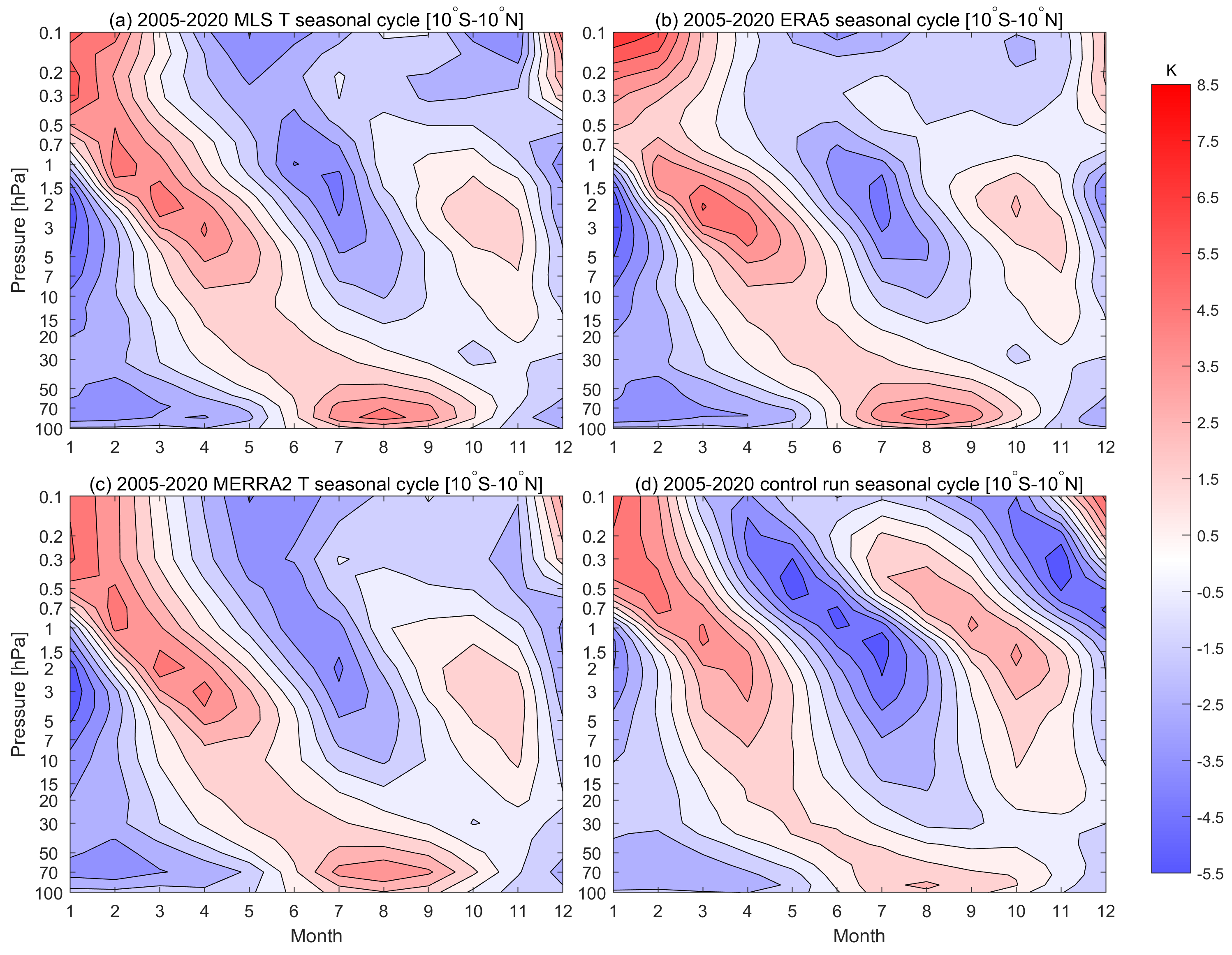
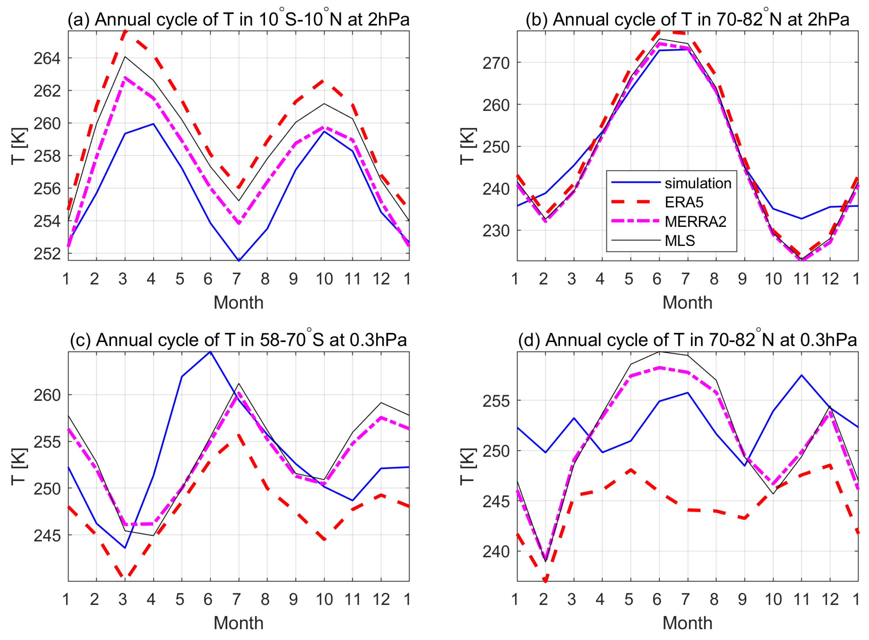
3.2. Time Analysis of the SAO

To analyze the temporal evolution of the SAO signals, four representative regions in the upper stratosphere and lower mesosphere around the peak of the SAO PSD are selected for further studies. To further analyze the variability of temperature data at different pressure levels, the linear trend of the temperature time series is removed. Figure 3 shows the monthly annual mean linearly detrended temperature variations from 100 to 0.1 hPa in the tropics (10 ° S–10 ° N). In the tropics, the SAO becomes dominated in the range 30–0.1 hPa and strongest around 3–1 hPa in all data sets (Figure 3). For 3–1 hPa, two warm spots in March–April and October and two cold spots in January and July are obvious in the tropical region. For 0.5–0.1 hPa, two cold spots occur in May and October–November in the tropics. A weaker magnitude of temperature SAO compared to annual magnitude is found in NH high latitudes in the upper stratosphere (Figure 2). In the NH and SH high latitudes, temperatures are becoming more and more dominated by the SAO in the range of 0.5–0.1 hPa (Figure 2).
The maximum tropical SAO is centered around 2 hPa and the SAO is observed in almost all latitude bands at 0.3 hPa in all data sets. Furthermore, they are not too close to the top level of reanalysis and are suitable for analyzing the possible effects. For these reasons, time series at 2 hPa and 0.3 hPa were chosen for further studies. Figure 4 shows the yearly climatological cycle of temperature in the tropics and NH high latitudes at 2 hPa and in the SH/NH high latitudes at 0.3 hPa. At 2 hPa, two temperature peaks are obvious in March and October in the tropical region. In contrast, the peak of the temperature in June–July is dominant at 2 hPa in the NH high latitudes (Figure 4b). The MERRA2 and MLS temperature time series are the most consistent across all data sets. The possible reason is that MERRA2 assimilates the MLS temperature above 5 hPa and the monthly binned MLS products use MERRA2 temperature fields for the interpolation. As described in the MLS document [34], the MLS profiles on pressure levels are first interpolated to fixed potential temperature surfaces before being binned. The annual climatological temperature cycle shown by the model simulation is in agreement with MLS and reanalysis data in this region.
In the lower mesosphere, two peaks are observed in July and December in the SH high latitudes (Figure 4c), which is nearly anti-correlated with the tropical SAO in the upper stratosphere (Figure 4a). In the SH high latitudes at 0.3 hPa, the model simulation shows two peaks in June and January, which is a month earlier than other data sets (Figure 4c). The difference between the simulation and other data sets should be due to the large uncertainty of simulations in the mesosphere. The NH high latitude temperature shows two peaks in June and December in the NH high latitudes at 0.3 hPa (Figure 4d). As shown in Figure 4d, the MLS and MERRA2 temperatures again have the best match in the NH high latitudes with two temperature peaks in June and December. However, there are substantial differences between ERA5 and MLS at 0.3 hPa in the NH high latitudes. In ERA5, two peaks are located in May and December and the first peak is much lower than the one of MERRA2/MLS in June. The possible reason for the difference is the observation-free mesosphere of ERA5 compared with MERRA2, which indicates an important role of satellite data assimilation for the representation of the SAO in the middle atmosphere. The largest differences are found between the simulation and other data sets in Figure 4d. Three local maximums and minimums in the yearly climatological cycle of temperature are observed in the simulation in the NH high latitudes at 0.3 hPa. Temperature differences between different data sets are more pronounced at 0.3 hPa than at 2 hPa. Particularly in the northern polar region, there are discrete mesospheric cooling events captured by MLS and reanalysis temperature time series, which are not found in most respects in simulations. The model simulation cannot simulate these strong cooling events, which could be the reason for different climatology with other data sets. In contrast, no such strong cooling events are observed in the temperature time series in the SH high latitudes; as a result, the temperature differences between the simulation and other data sets are smaller than those in NH high latitudes (Figure 4c,d).

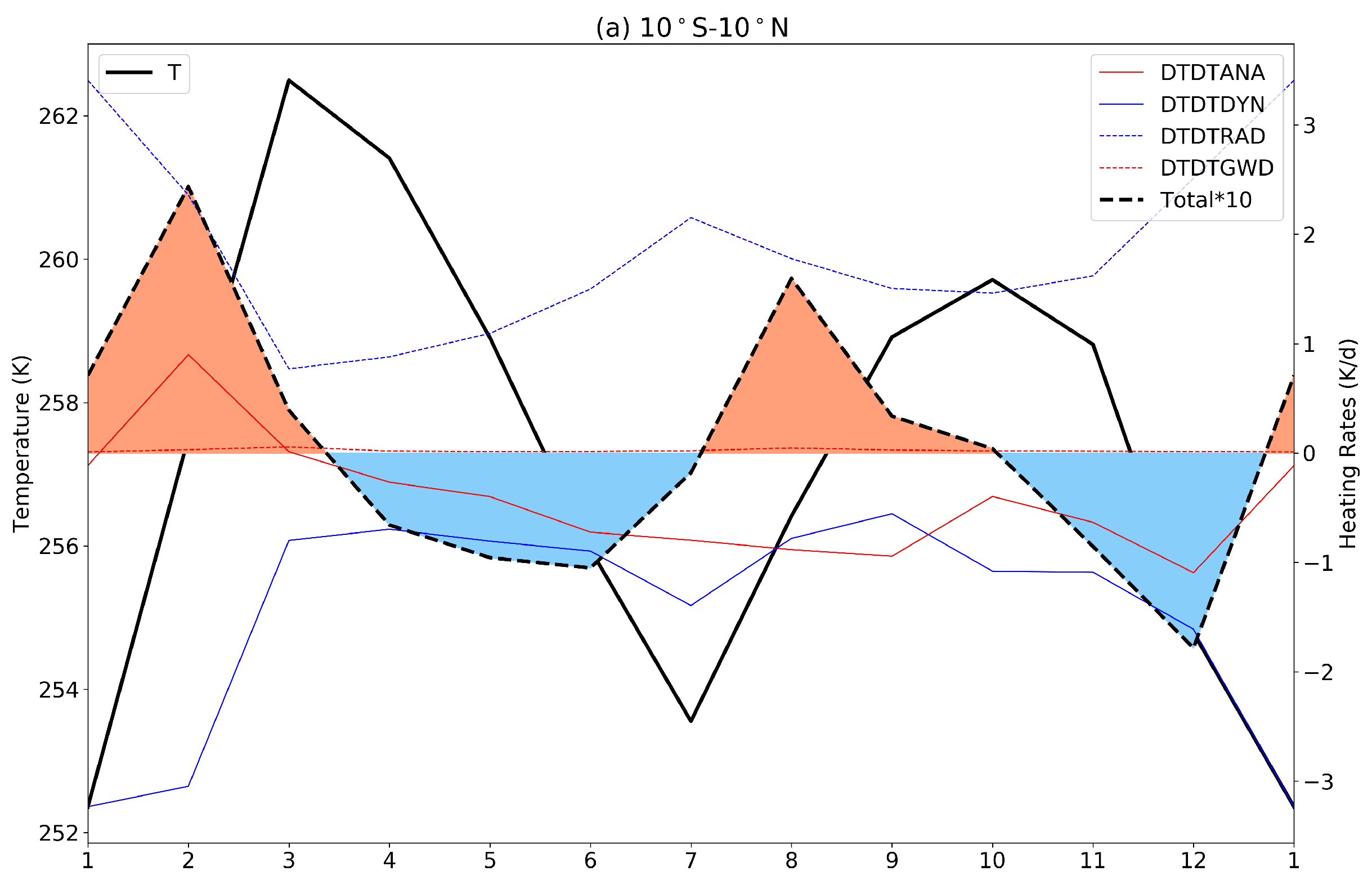
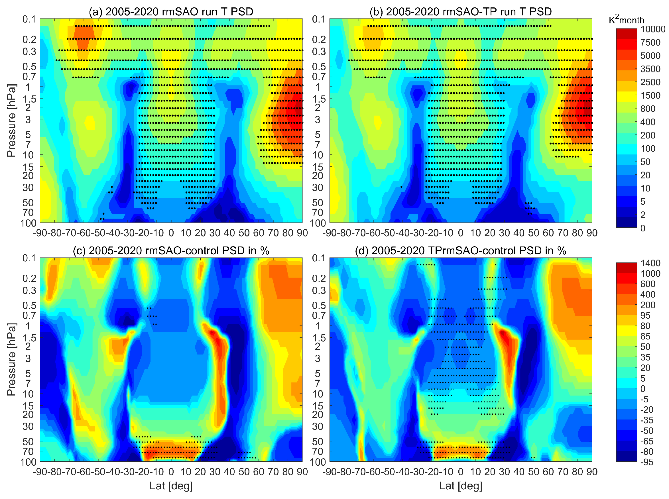
3.3. Mechanism of the SAO

The heating rates (temperature tendency) indicate how the temperature is changed and therefore are helpful for understanding the processes determining the temperature changes. To better understand the mechanism of the SAO in the middle atmosphere, the monthly heating rates of MERRA2 and model simulations in the corresponding region are analyzed. To clearly show the relative contribution of different terms to the total heating rate, the variation of each term at highs and lows of total heating rates is selected and is shown in Figure 5 and Figure 6. The annual cycle of the MERRA2 temperature is also shown together with heating rates to study the mechanism of the SAO.
As one of the most important radiative gases, ozone is very important to the temperature variations in the middle atmosphere. In addition, ozone in the middle atmosphere exhibits an SAO associated with SAO in the tropical zonal wind and temperature [53]. Therefore, we show the corresponding MLS annual cycle of ozone and temperature in the same region to study the relative effects of dynamics and chemistry (Figure 7).
In the tropics, there are two peaks in total heating rates around February and August and two nadirs around December and June (Figure 5a). As shown in Figure 5a, the total heating rates are positive from mid-December to mid-March and from July to October, which leads to a rise in temperature over the same period. From mid-March and July, the total heating rates are negative and the temperature decreases simultaneously. As a consequence, two peaks of the temperature in March and October and two nadirs in January and July are found at 2 hPa in the tropics. A similar pattern is also found in the simulation (not shown here). In the tropics, the stratosphere is heated mainly by the absorption of solar ultraviolet radiation by ozone. Ozone in the tropics at 2 hPa shows two peaks in January and July (Figure 7a). This makes the radiative heating rates also peak in January and July (Figure 5a). However, due to the strong dynamical cooling effects, the total heating rates show two peaks in February and August. The temperature increases while the total heating rates are positive, which makes the temperature peaks delay to the total heating rates. The temperature time series shows mainly anti-correlated (−0.97) with MLS ozone in the tropics. The reason for the negative correlation between ozone and temperature is that the photochemical reactions of ozone depend inversely on the temperature [54,55]. According to SPARC Data Initiative [53], a tropical SAO with asymmetric amplitudes is found at 10 hPa by the ozone observations. The amplitude of SAO at 2 hPa is also stronger in the first half of the calendar year (Figure 7). The two peaks in temperature are asymmetrical due to the different ozone concentrations. In Figure 5a, the temperature in January is colder than in July. Our study shows that the dynamical processes contribute the most prominent negative heating rates through all terms, which is mostly offset by radiative warming. The dynamical cooling is found to be strongest in January, which could be the reason for the lowest temperature in January. The temperature peaks in March and October are mainly related to radiative heating since the dynamical terms are negative.
In the NH high latitudes at 2 hPa, both the radiative cooling and dynamical warming are strongest around January (Figure 5b). The strongest radiative warming occurs in May and the strongest dynamical cooling occurs in June. The radiative and dynamical terms show an opposite sign in this region. The total heating rates are positive from mid-February to mid-June and from November to mid-January, as shown in Figure 5b. When the total heating rate is positive, the temperature increases meanwhile. The temperature peak in July is mainly determined by a combination of dynamical and radiative warming and the temperature peak in January is mainly related to dynamical terms. The polar stratospheric warming and the Brewer–Dobson circulation (BDC) might affect the SAO in the northern polar region [10,11]. An out-of-phase relationship between tropical and NH high-latitude SAO is found in the upper stratosphere (Figure 5a,b). Ref. [11] found this relationship in the upper stratosphere could be related to the variability in the strength of BDC. According to the SPARC report [53], the Canadian Middle Atmosphere Model (CMAM30) also captures distinct methane SAO at 10 and 2 hPa in the tropical and polar regions. However, the SAO in the polar region at 10 hPa is related to BDC while the SAO at 2 hPa is a result of photochemistry [56,57]. In the NH high latitudes, the MLS ozone time series also exhibits a semi-annual variation (Figure 7b), which shows a strong negative correlation (−0.76) with temperature. According to [54], the ozone depletion rate increases due to the warm summer temperature, which causes the ozone concentration to decrease after March. The temperature starts to decrease after July and the ozone starts to increase due to the decrease in ozone destruction processes. The radiative heating rates are also changed along with the ozone concentration. Therefore, the temperature SAO in this region also has a connection with ozone SAO [54]. For the simulation (not shown here), the total heating rates are positive from January to mid-June and from mid-October to mid-November and are negative from mid-June to mid-October and from mid-November to January, which is similar to the MERRA2.
In the SH high latitudes at 0.3 hPa (Figure 6a), the total heating rates are positive from mid-March to mid-June and from mid-September to December, which leads to the first peak of temperature in July and the second peak in December. The first temperature peak in July is mainly due to strong dynamical warming while the second temperature peak in December is mainly due to strong radiative warming. Unlike the NH high latitudes and the tropics in the stratosphere, the correlation of time series between ozone and temperature in this region is weaker (−0.54) (Figure 7c). However, large positive dynamical terms are found in Figure 6a and the reason for this is not clear. In the simulation (not shown here), the positive heating rates are from mid-February to mid-May and from mid-October to mid-December, which is a month earlier end than those of MERRA2. Therefore, the temperature peaks and nadirs shown in the simulation are also a month earlier compared with MERRA2.
In the NH high latitudes at 0.3 hPa (Figure 6b), the total heating rates are positive from mid-January to June and from mid-September to mid-November with temperature peaks in June and December. Negative heating rates are observed from June to mid-September and from mid-November to mid-January with two nadirs in October and February. The first temperature peak in June is much higher than that in December. The first peak in June is mainly related to the combination warming of radiative and dynamical terms, while the second peak in December is mainly related to the strong dynamical warming. The climatological cycle of ozone is highest in February and November and lowest in June and December (Figure 7d). The MLS ozone is also strongly anti-correlated (−0.89) with the temperature in this region. The strong correlation between temperature and ozone variations is similar to the case at 2 hPa, which confirms the importance of chemistry and dynamics to the SAO in the NH high latitudes. This also indicates that the correlation between temperature and ozone varies in the SH and NH high latitudes in the lower mesosphere. For the simulation, the variation in heating rates does not agree with the annual cycle of the simulation temperature (not shown here), which could be caused by larger uncertainties in the simulation in the mesosphere due to larger dynamical variability in particular in the NH high latitudes [53].

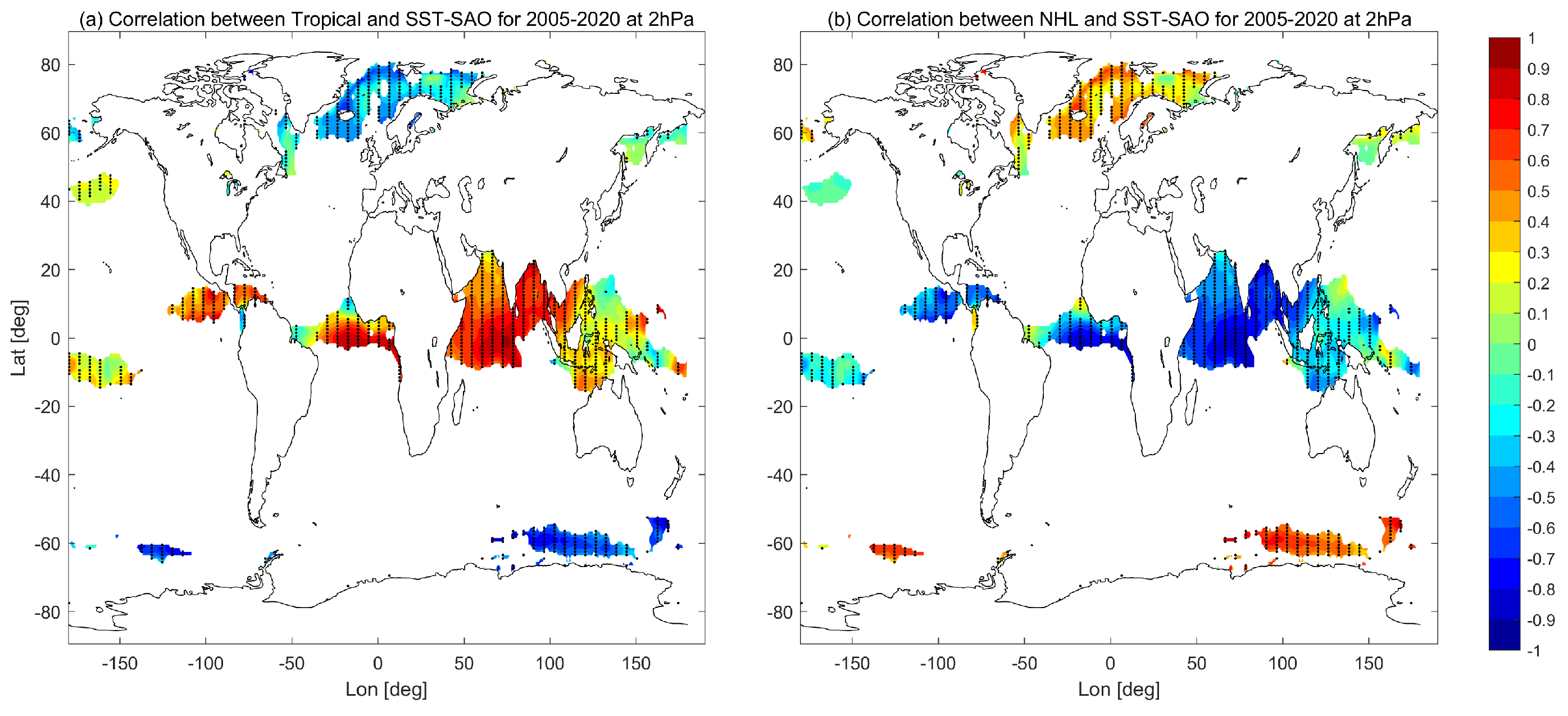
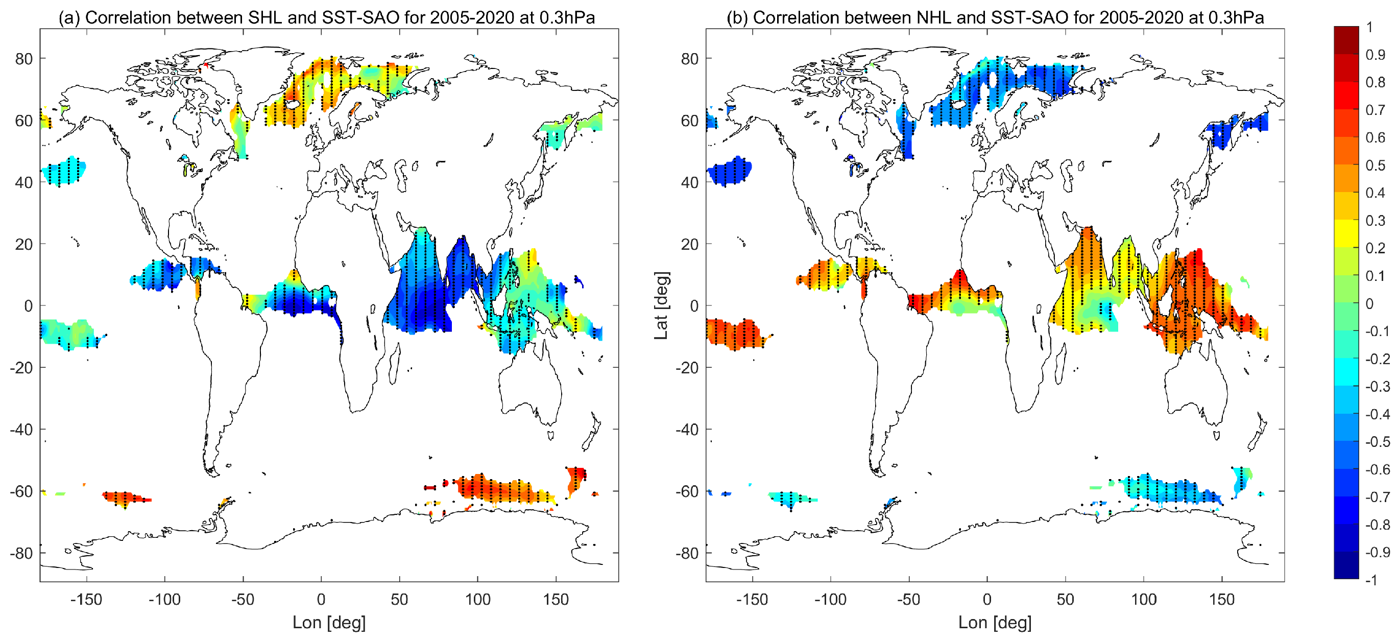
3.4. Relationship between the SAO and SSTs

The pronounced SAO signal is observed at the surface and is coupled with atmosphere [58]. Therefore, it is useful to examine the relationship between the SAO in the middle atmosphere and the surface SAO. Since the SST may modify the atmospheric circulation and affect the temperature in the middle atmosphere subsequently. We first check the correlation between the temperature SAO in the middle atmosphere and SST-SAO to show the possibility of the connection between them and use the model simulations to further check the possible responses of temperature SAO in the middle atmosphere to SST-SAO. MLS temperature SAO signals (5–7 months) and SST-SAO (5–7 months) were extracted using the 1D wavelet Morlet transform.
Many studies [24,59,60] have found that SST-SAO signals are significant in the tropics from the Western Pacific (150 ° E), the Indian Ocean and the Atlantic Ocean to the Eastern Pacific (120 ° W). In the NH and SH high latitudes, the significant SAO region is located at the Antarctic Ocean (85 ° E–150 ° E) around 60 ° S and around 60 ° W–60 ° E from the North Atlantic Ocean (60 ° N) to the Arctic Ocean (80 ° N), whose area is much smaller than that in the tropics. The correlation is calculated between the time series of the area-averaged temperature SAO (e.g., 10 ° S–10 ° N at 2 hPa, taking only the SAO component) and the SST-SAO time series at each grid point. (Figure 8 and Figure 9). The dots in Figure 8 and Figure 9 indicate that the correlation coefficient is significant at the 5% level. Significant correlation coefficients in high latitudes and the tropics always have an inverse sign in general (Figure 8 and Figure 9). As shown in Figure 8, both tropical SAO and NH high latitude SAO at 2 hPa show a strong correlation with SST-SAO in most of the regions but with an opposite sign. It corresponds to the out-of-phase relationship between the SAO in the tropics and high latitudes in the upper stratosphere. At 0.3 hPa the correlation between SAO in SH/NH high latitudes and SST-SAO is also strong but with an opposite sign of each other. This indicates that the SAO in the NH high latitudes at 0.3 hPa is also not in sync with the SAO in the SH high latitudes at 0.3 hPa.
As described above, the temperature SAO in the middle atmosphere has high correlation with the SST-SAO. For further analysis, we have performed three simulations (rmSAO, rmSAO-TP and control runs) with different prescribed SSTs as described in Section 2.3. Figure 10 shows the PSD of the SAO in temperature based on rmSAO and rmSAO-TP runs, as well as their relative differences to the control run. There are similar significant SAO regions in rmSAO and rmSAO-TP simulations. Both SAO PSD of rmSAO and rmSAO-TP simulations become smaller in the tropics around 15–0.1 hPa and larger in high latitudes (the Arctic Pole around 10–0.2 hPa and SH high latitudes around 0.5–0.1 hPa). This confirms that the SST-SAO has an opposite relationship with SAO in the tropical and polar regions. When the SST-SAO is removed globally, the magnitude of the rmSAO run decreased in SH high latitudes between 0.5 and 0.1 hPa and in the northern polar region between 20 and 5 hPa compared to the rmSAO-TP run. This suggests that SST-SAO in high latitudes shows a higher correlation with these regions. It confirms that the different features of SAO in the middle atmosphere could be at least partially due to the SST-SAO.
The differences in the simulation energy budget are shown in Figure 11 and Figure 12. At 2 hPa, a reduction of the averaged amplitude of total heating rates is observed by the rmSAO and rmSAO-TP compared with the control run in the tropical region but an increase in the NH high latitudes (Figure 11). Solar radiation is one of the main engines of the SST-SAO and stratospheric SAO in the tropics. Therefore, the amplitude is reduced by removing the SST-SAO in the simulation. The opposite change of total heating rates in the NH high latitudes and tropical regions by removing the SST-SAO could be related to anti-correlation between the tropics and high latitude upper stratospheric temperature SAO as shown in Figure 8. This out-of-phase relationship is a response to the variability in the strength of the Brewer–Dobson circulation and photochemistry [11,56,57]. The mean SAO signal extracted from MERRA2 observations shows a similar pattern with SAO signals of simulations at 2 hPa. An anti-correlation between tropical and NH high latitude temperature SAO in the stratosphere is presented in simulations.
At 0.3 hPa, there is also an increase in the amplitude of the total hearing rates in the NH high latitudes (Figure 12). However, in the SH high latitudes, the change in the total heating rates is smaller than in the NH high latitudes. The MERRA2 heating rates in the NH high latitudes is different from that of simulations (Figure 4). The large difference in temperature and heating rates between MERRA2 and simulations at 0.3 hPa could cause large uncertainty in the model simulation, which leads to difficulty in simulating a realistic SAO in the lower mesosphere. The experiment also confirms that the SST-SAO has affected the SAO of temperature in the middle atmosphere, particularly in the upper stratosphere and SH high latitudes in the lower mesosphere. Further analysis is required for the NH high latitude SAO in the lower mesosphere due to the large uncertainties of model simulations in this region.

4. Conclusions

The SAO in the middle atmosphere is a primary variation of global temperature, which plays an important role in numerical weather prediction and climate research [61,62]. MLS, ERA5, MERRA2 and WACCM simulations are used to study the spatio-temporal variation of the SAO in the upper stratosphere and lower mesosphere in this paper. This analysis finds evidence of SAO of temperature in the tropical region (20 ° S–20 ° N) with a peak around 1–3 hPa, which is consistent with previous studies. In addition, we found that SAO is also significant in the NH high latitudes between 8 and 0.3 hPa and SH high latitudes between 0.5 and 0.1 hPa, which has been less of a concern in previous studies. Significant SAO regions extend to most of the latitudes in the lower mesosphere. For all four data sets, MERRA2 and MLS have the best agreement in general. ERA5 also has good agreement with MLS data in the stratosphere but differences in the mesosphere. According to the result, MERRA2 benefited from the assimilation of MLS observations above 5 hPa, which provided a constraint on the dynamics especially in the lower mesosphere. Large differences in the lower mesosphere between the simulation and other data sets are found because of large uncertainties in the model simulation, especially in the NH high latitudes. The results of our study could provide a good reference for the SPARC community and reanalysis centers. In particular, the comprehensive view of the SAO based on satellite, reanalyses and model simulations provide valuable information as there is a lack of study on the SAO in the lower mesosphere high latitudes.
An important new result from this study is the relationship between temperature SAO and MERRA2 thermal energy budget. The tropical SAO in the stratosphere is mainly related to radiative processes. The seasonal change of ozone concentration led to two radiative warming peaks in January and July. The significant SAO in the northern polar region (70 ° N–90 ° N) is mainly related to a combination of dynamical and radiative processes. According to the energy budget analysis at 2 hPa, the temperature peak in July in the NH latitudes is mainly determined by a combination of dynamical and radiative processes and the peak in January is mainly due to dynamical processes. At 0.3 hPa, the first peak in June is mainly associated with dynamical and radiative warming and the second peak in December is mainly associated with strong dynamical warming. The strong anti-correlation between temperature and ozone confirms there is an important relationship between chemistry and dynamics in the NH high latitudes and tropics. In SH high latitudes of the lower mesosphere, the temperature is also anti-correlated with ozone but with a lower value compared with other regions. The main difference of the ozone and temperature relationship in the SH can be seen in April and May, which shows a delay of the ozone peak in May to the lowest temperature in April. The exact reason for this delay awaits further studies. This indicates the relationship between ozone and temperature varies in the SH and NH high latitudes in the lower mesosphere. The first temperature peak in July in the SH high latitudes is due to strong dynamical warming while the second peak in December is related to strong radiative warming. The energy budget of the simulation shows a good agreement with MERRA2 in the upper stratosphere but obvious differences in the lower mesosphere especially in the NH high latitudes. Large differences in temperature and heating rates between the simulation and other data sets indicate that the model simulation has difficulty in simulating a realistic SAO in the lower mesosphere. The good agreement between MERRA2 and simulation in the upper stratosphere confirms that the model could at least partially represent the right dynamical mechanisms that produce the SAO in the middle atmosphere.
We also investigate the relationship between the temperature SAO in the middle atmosphere and SST-SAO. The correlation coefficients between SAO in the middle atmosphere and SST-SAO show an opposite sign in the tropics and high latitudes. In the lower mesosphere, the correlation coefficients between the SH/NH high latitudes and SST-SAO also show a different sign. By removing SST-SAO, the magnitude of the SAO decreases in the tropics and increases in the polar region. To some extent, these differences indicate the temperature response to different SST conditions. This confirmed the link between SST-SAO and temperature SAO in the middle atmosphere. However, the NH high latitude SAO in the lower mesosphere is not significant by the model simulation. Further analysis is needed to study the SAO in the lower mesosphere with more observations and model development in the future, especially in high latitudes.

Author Contributions

Conceptualization, M.S.; methodology, validation, formal analysis, investigation, resources, data curation, visualization, funding acquisition, M.S. and W.W.; writing—original draft preparation, M.S.; writing—review and editing, W.W. All authors have read and agreed to the published version of the manuscript.

Funding

This research was funded by the National Natural Science Foundation of China (Grant No. 41904023 and 42075055) and the Fundamental Research Funds for the Central Universities, China University of Geosciences (Wuhan) (Grant No. CUG2106357).

Data Availability Statement

The MERRA2 data is available from the NASA GSFC (https://disc.gsfc.nasa.gov/datasets?project=MERRA-2, accessed on 18 July 2022). The ERA5 data is available from the Copernicus Climate Change Service (https://cds.climate.copernicus.eu, accessed on 18 July 2022). The simulations can be provided to readers by contacting the corresponding author.

Acknowledgments

We thank the NASA GSFC, for providing the MLS data and MERRA2 data, Copernicus Climate Change Service and ECMWF, for the ERA5 data, and NCAR, for the CESM-WACCM model. We thank the three reviewers and the editor, for the very helpful comments and suggestions.

Conflicts of Interest

The authors declare no conflict of interest.

References

  1. Labitzke, K.; Barnett, J.J. Global time and space changes of satellite radiances received from the stratosphere and lower mesosphere. J. Geophys. Res. 1973, 78, 483–496. [Google Scholar] [CrossRef]
  2. Chandra, S.; Fleming, E.L.; Schoeberl, M.R.; Barnett, J.J. Monthly mean global climatology of temperature, wind, geopotential height and pressure for 0–120 km. Adv. Space Res. 1990, 10, 3–12. [Google Scholar] [CrossRef]
  3. Ern, M.; Diallo, M.; Preusse, P.; Mlynczak, M.G.; Schwartz, M.J.; Wu, Q.; Riese, M. The semiannual oscillation (SAO) in the tropical middle atmosphere and its gravity wave driving in reanalyses and satellite observations. Atmos. Chem. Phys. 2021, 21, 13763–13795. [Google Scholar] [CrossRef]
  4. REED, R.J. Some Features of the annual temperature regime in the tropical stratosphere. Mon. Weather Rev. 1962, 90, 211–215. [Google Scholar] [CrossRef]
  5. Reed, R.J. Zonal wind behavior in the equatorial stratosphere and lower mesosphere. J. Geophys. Res. 1966, 71, 4223–4233. [Google Scholar] [CrossRef]
  6. Volland, H. A theory of thermospheric dynamics—II: Geomagnetic activity effect, 27-day variation and semiannual variation. Planet. Space Sci. 1969, 17, 1709–1724. [Google Scholar] [CrossRef]
  7. van Loon, H.; Labitzke, K.; Jenne, R.L. Half-yearly wave in the stratosphere. J. Geophys. Res. 1972, 77, 3846–3855. [Google Scholar] [CrossRef]
  8. Hirota, I. Observational evidence of the semiannual oscillation in the tropical middle atmosphere—A review. Pure Appl. Geophys. 1980, 118, 217–238. [Google Scholar] [CrossRef]
  9. Zhang, Y.; Sheng, Z.; Shi, H.; Zhou, S.; Shi, W.; Du, H.; Fan, Z. Properties of the Long-Term Oscillations in the Middle Atmosphere Based on Observations from TIMED/SABER Instrument and FPI over Kelan. Atmosphere 2017, 8, 7. [Google Scholar] [CrossRef]
  10. Gao, X.H.; Yu, W.B.; Stanford, J.L. Global Features of the Semiannual Oscillation in Stratospheric Temperatures and Comparison between Seasons and Hemispheres. J. Atmos. Sci. 1987, 44, 1041–1048. [Google Scholar] [CrossRef]
  11. Young, P.J.; Thompson, D.W.J.; Rosenlof, K.H.; Solomon, S.; Lamarque, J.F. The Seasonal Cycle and Interannual Variability in Stratospheric Temperatures and Links to the Brewer–Dobson Circulation: An Analysis of MSU and SSU Data. J. Clim. 2011, 24, 6243–6258. [Google Scholar] [CrossRef]
  12. Ganguly, S. Semiannual variations in the mesosphere. J. Geophys. Res. 1975, 80, 3722–3724. [Google Scholar] [CrossRef]
  13. Hamilton, K. Rocketsonde observations of the mesospheric semiannual oscillation at Kwajalein. Atmos.-Ocean 1982, 20, 281–286. [Google Scholar] [CrossRef]
  14. Dunkerton, T.J. Theory of the Mesopause Semiannual Oscillation. J. Atmos. Sci. 1982, 39, 2681–2690. [Google Scholar] [CrossRef]
  15. Sassi, F.; Garcia, R.R. The Role of Equatorial Waves Forced by Convection in the Tropical Semiannual Oscillation. J. Atmos. Sci. 1997, 54, 1925–1942. [Google Scholar] [CrossRef]
  16. Richter, J.H.; Garcia, R.R. On the forcing of the Mesospheric Semi-Annual Oscillation in the Whole Atmosphere Community Climate Model. Geophys. Res. Lett. 2006, 33, L01806. [Google Scholar] [CrossRef]
  17. Lossow, S.; Urban, J.; Gumbel, J.; Eriksson, P.; Murtagh, D. Observations of the mesospheric semi-annual oscillation (MSAO) in water vapour by Odin/SMR. Atmos. Chem. Phys. 2008, 8, 6527–6540. [Google Scholar] [CrossRef]
  18. Mayr, H.; Mengel, J.; Chan, K.; Huang, F. Middle atmosphere dynamics with gravity wave interactions in the numerical spectral model: Zonal-mean variations. J. Atmos. Sol.-Terr. Phys. 2010, 72, 807–828. [Google Scholar] [CrossRef]
  19. Smith, A.K.; Holt, L.A.; Garcia, R.R.; Anstey, J.A.; Serva, F.; Butchart, N.; Osprey, S.; Bushell, A.C.; Kawatani, Y.; Kim, Y.H.; et al. The equatorial stratospheric semiannual oscillation and time-mean winds in QBOi models. Q. J. R. Meteorol. Soc. 2020, 148, 1593–1609. [Google Scholar] [CrossRef]
  20. Huang, F.T.; Mayr, H.G.; Reber, C.A.; Russell, J.M.; Mlynczak, M.; Mengel, J.G. Stratospheric and mesospheric temperature variations for the quasi-biennial and semiannual (QBO and SAO) oscillations based on measurements from SABER (TIMED) and MLS (UARS). Ann. Geophys. 2006, 24, 2131–2149. [Google Scholar] [CrossRef] [Green Version]
  21. Smith, A.K.; Garcia, R.R.; Moss, A.C.; Mitchell, N.J. The Semiannual Oscillation of the Tropical Zonal Wind in the Middle Atmosphere Derived from Satellite Geopotential Height Retrievals. J. Atmos. Sci. 2017, 74, 2413–2425. [Google Scholar] [CrossRef]
  22. Zhao, X.R.; Sheng, Z.; Shi, H.Q.; Weng, L.B.; He, Y. Middle Atmosphere Temperature Changes Derived from SABER Observations during 2002–20. J. Clim. 2021, 34, 7995–8012. [Google Scholar] [CrossRef]
  23. Long, C.S.; Fujiwara, M.; Davis, S.; Mitchell, D.M.; Wright, C.J. Climatology and interannual variability of dynamic variables in multiple reanalyses evaluated by the SPARC Reanalysis Intercomparison Project (S-RIP). Atmos. Chem. Phys. 2017, 17, 14593–14629. [Google Scholar] [CrossRef]
  24. Shangguan, M.; Wang, W. The semi-annual oscillation (SAO) in the upper troposphere and lower stratosphere (UTLS). Atmos. Chem. Phys. 2022, 22, 9499–9511. [Google Scholar] [CrossRef]
  25. Thompson, D.W.J.; Baldwin, M.P.; Wallace, J.M. Stratospheric Connection to Northern Hemisphere Wintertime Weather: Implications for Prediction. J. Clim. 2002, 15, 1421–1428. [Google Scholar] [CrossRef]
  26. Charlton-Perez, A.J.; Baldwin, M.P.; Birner, T.; Black, R.X.; Butler, A.H.; Calvo, N.; Davis, N.A.; Gerber, E.P.; Gillett, N.; Hardiman, S.; et al. On the lack of stratospheric dynamical variability in low-top versions of the CMIP5 models. J. Geophys. Res. Atmos. 2013, 118, 2494–2505. [Google Scholar] [CrossRef]
  27. Gettelman, A.; Mills, M.J.; Kinnison, D.E.; Garcia, R.R.; Smith, A.K.; Marsh, D.R.; Tilmes, S.; Vitt, F.; Bardeen, C.G.; McInerny, J.; et al. The Whole Atmosphere Community Climate Model Version 6 (WACCM6). J. Geophys. Res. Atmos. 2019, 124, 12380–12403. [Google Scholar] [CrossRef]
  28. Marsh, D.R.; Mills, M.J.; Kinnison, D.E.; Lamarque, J.F.; Calvo, N.; Polvani, L.M. Climate Change from 1850 to 2005 Simulated in CESM1(WACCM). J. Clim. 2013, 26, 7372–7391. [Google Scholar] [CrossRef]
  29. Schoeberl, M.; Douglass, A.; Hilsenrath, E.; Bhartia, P.; Beer, R.; Waters, J.; Gunson, M.; Froidevaux, L.; Gille, J.; Barnett, J.; et al. Overview of the EOS aura mission. IEEE Trans. Geosci. Remote Sens. 2006, 44, 1066–1074. [Google Scholar] [CrossRef]
  30. Waters, J.; Froidevaux, L.; Harwood, R.; Jarnot, R.; Pickett, H.; Read, W.; Siegel, P.; Cofield, R.; Filipiak, M.; Flower, D.; et al. The Earth observing system microwave limb sounder (EOS MLS) on the aura Satellite. IEEE Trans. Geosci. Remote Sens. 2006, 44, 1075–1092. [Google Scholar] [CrossRef]
  31. Livesey, N.J.; Read, W.G.; Froidevaux, L.; Lambert, A.; Santee, M.L.; Schwartz, M.J.; Millán, L.F.; Jarnot, R.F.; Wagner, P.A.; Hurst, D.F.; et al. Investigation and amelioration of long-term instrumental drifts in water vapor and nitrous oxide measurements from the Aura Microwave Limb Sounder (MLS) and their implications for studies of variability and trends. Atmos. Chem. Phys. 2021, 21, 15409–15430. [Google Scholar] [CrossRef]
  32. Schwartz, M.J.; Lambert, A.; Manney, G.L.; Read, W.G.; Livesey, N.J.; Froidevaux, L.; Ao, C.O.; Bernath, P.F.; Boone, C.D.; Cofield, R.E.; et al. Validation of the Aura Microwave Limb Sounder temperature and geopotential height measurements. J. Geophys. Res. Atmos. 2008, 113, D15S11. [Google Scholar] [CrossRef]
  33. Lee, J.N.; Wu, D.L. Solar Cycle Modulation of Nighttime Ozone Near the Mesopause as Observed by MLS. Earth Space Sci. 2020, 7, e2019EA001063. [Google Scholar] [CrossRef]
  34. Livesey, N.; Coauthors. Earth Observing System (EOS) Aura Microwave Limb Sounder (MLS) Version 5.0x Level 2 and 3 data quality and description document. JPL Tech. Rep. 2022, JPL D-105336 Rev. B, 168–171. [Google Scholar]
  35. Hersbach, H.; Bell, B.; Berrisford, P.; Hirahara, S.; Horányi, A.; Muñoz-Sabater, J.; Nicolas, J.; Peubey, C.; Radu, R.; Schepers, D.; et al. The ERA5 global reanalysis. Q. J. R. Meteorol. Soc. 2020, 146, 1999–2049. [Google Scholar] [CrossRef]
  36. Gelaro, R.; McCarty, W.; Suárez, M.J.; Todling, R.; Molod, A.; Takacs, L.; Randles, C.A.; Darmenov, A.; Bosilovich, M.G.; Reichle, R.; et al. The Modern-Era Retrospective Analysis for Research and Applications, Version 2 (MERRA-2). J. Clim. 2017, 30, 5419–5454. [Google Scholar] [CrossRef]
  37. Hersbach, H.; Bell, B.; Berrisford, P.; Biavati, G.; Horányi, A.; Muñoz Sabater, J.; Nicolas, J.; Peubey, C.; Radu, R.; Rozum, I.; et al. ERA5 monthly averaged data on pressure levels from 1979 to present. Copernicus Climate Change Service (C3S) Climate Data Store (CDS). 2019. Available online: https://cds.climate.copernicus.eu/cdsapp#!/dataset/10.24381/cds.6860a573?tab=overview (accessed on 18 July 2022).
  38. GMAO. Global Modeling and Assimilation Office, instM_3d_asm_Np: MERRA2 3D IAU State, Meteorology Monthly Mean, Version 5.12.4, Greenbelt, MD, USA: Goddard Space Flight Center Distributed Active Archive Center (GSFC DAAC) 2015. Available online: https://disc.gsfc.nasa.gov/datasets/M2IMNPASM_5.12.4/summary (accessed on 18 July 2022).
  39. GMAO. Global Modeling and Assimilation Office, tavgM_3d_tdt_Np: MERRA2 3D IAU State, Meteorology Monthly Mean, Version 5.12.4, Greenbelt, MD, USA: Goddard Space Flight Center Distributed Active Archive Center (GSFC DAAC) 2015. Available online: https://disc.gsfc.nasa.gov/datasets/M2TMNPTDT_5.12.4/summary (accessed on 18 July 2022).
  40. Fujiwara, M.; Wright, J.S.; Manney, G.L.; Gray, L.J.; Anstey, J.; Birner, T.; Davis, S.; Gerber, E.P.; Harvey, V.L.; Hegglin, M.I.; et al. Introduction to the SPARC Reanalysis Intercomparison Project (S-RIP) and overview of the reanalysis systems. Atmos. Chem. Phys. 2017, 17, 1417–1452. [Google Scholar] [CrossRef]
  41. Rayner, N.A.; Parker, D.E.; Horton, E.B.; Folland, C.K.; Alexander, L.V.; Rowell, D.P.; Kent, E.C.; Kaplan, A. Global analyses of sea surface temperature, sea ice and night marine air temperature since the late nineteenth century. J. Geophys. Res. Atmos. 2003, 108, 4407. [Google Scholar] [CrossRef]
  42. Matthes, K.; Funke, B.; Andersson, M.E.; Barnard, L.; Beer, J.; Charbonneau, P.; Clilverd, M.A.; Dudok de Wit, T.; Haberreiter, M.; Hendry, A.; et al. Solar forcing for CMIP6 (v3.2). Geosci. Model Dev. 2017, 10, 2247–2302. [Google Scholar] [CrossRef]
  43. Butterworth, S. In the theory of filter amplifires. Exp. Wirel. Wirel. Eng. 1930, 7, 536–5413. [Google Scholar]
  44. Andrews, D.G.; Holton, J.R.; Leovy, C.B. Middle Atmopshere Dynamics; Academic Press: Orlando, FL, USA, 1987; p. 489. [Google Scholar]
  45. Abalos, M.; Randel, W.J.; Kinnison, D.E.; Serrano, E. Quantifying tracer transport in the tropical lower stratosphere using WACCM. Atmos. Chem. Phys. 2013, 13, 10591–10607. [Google Scholar] [CrossRef]
  46. Mapes, B.E.; Bacmeister, J.T. Diagnosis of Tropical Biases and the MJO from Patterns in the MERRA Analysis Tendency Fields. J. Clim. 2012, 25, 6202–6214. [Google Scholar] [CrossRef]
  47. Auger, F.; Flandrin, P. Improving the readability of time-frequency and time-scale representations by the reassignment method. IEEE Trans. Signal Process. 1995, 43, 1068–1089. [Google Scholar] [CrossRef]
  48. Fulop, S.A.; Fitz, K. Algorithms for computing the time-corrected instantaneous frequency (reassigned) spectrogram, with applications. J. Acoust. Soc. Am. 2006, 119, 360–371. [Google Scholar] [CrossRef]
  49. Wichert, S.; Fokianos, K.; Strimmer, K. Identifying periodically expressed transcripts in microarray time series data. Bioinformatics 2004, 20, 5–20. [Google Scholar] [CrossRef] [PubMed]
  50. Lilly, J.M.; Olhede, S.C. Higher-Order Properties of Analytic Wavelets. IEEE Trans. Signal Process. 2009, 57, 146–160. [Google Scholar] [CrossRef]
  51. Lilly, J.M.; Olhede, S.C. Generalized Morse Wavelets as a Superfamily of Analytic Wavelets. IEEE Trans. Signal Process. 2012, 60, 6036–6041. [Google Scholar] [CrossRef]
  52. Kawatani, Y.; Hirooka, T.; Hamilton, K.; Smith, A.K.; Fujiwara, M. Representation of the equatorial stratopause semiannual oscillation in global atmospheric reanalyses. Atmos. Chem. Phys. 2020, 20, 9115–9133. [Google Scholar] [CrossRef]
  53. Hegglin, M.I.; Tegtmeier, S. The SPARC Data Initiative: Assessment of Stratospheric Trace Gas and Aerosol Climatologies from Satellite Limb Sounders. Report, 2017. SPARC Report No. 8, WCRP-05/2017. Available online: https://www.research-collection.ethz.ch/handle/20.500.11850/156244 (accessed on 17 January 2023). [CrossRef]
  54. Perliski, L.M.; Solomon, S.; London, J. On the interpretation of seasonal variations of stratospheric ozone. Planet. Space Sci. 1989, 37, 1527–1538. [Google Scholar] [CrossRef]
  55. Huang, F.T.; Mayr, H.G.; Reber, C.A.; Russell, J.M., III; Mlynczak, M.G.; Mengel, J.G. Ozone quasi-biennial oscillations (QBO), semiannual oscillations (SAO) and correlations with temperature in the mesosphere, lower thermosphere and stratosphere, based on measurements from SABER on TIMED and MLS on UARS. J. Geophys. Res. 2008, 113, A01316. [Google Scholar] [CrossRef]
  56. Randel, W.J.; Wu, F.; Russell, J.M.; Roche, A.; Waters, J.W. Seasonal Cycles and QBO Variations in Stratospheric CH4 and H2O Observed in UARS HALOE Data. J. Atmos. Sci. 1998, 55, 163–185. [Google Scholar] [CrossRef]
  57. Solomon, S.; Garcia, R.; Rowland, F.; Wuebbles, D. On the depletion of Antarctic ozone. Nature 1986, 321, 755–758. [Google Scholar] [CrossRef]
  58. Meehl, G.A.; Hurrell, J.W.; Loon, H.V. A modulation of the mechanism of the semiannual oscillation in the Southern Hemisphere. Tellus A 1998, 50, 442–450. [Google Scholar] [CrossRef]
  59. Park, K.A.; Lee, E.Y. Semi-annual cycle of sea-surface temperature in the East/Japan Sea and cooling process. Int. J. Remote Sens. 2014, 35, 4287–4314. [Google Scholar] [CrossRef]
  60. Yan, Y.; Wang, G.; Chen, C.; Ling, Z. Annual and Semiannual Cycles of Diurnal Warming of Sea Surface Temperature in the South China Sea. J. Geophys. Res. 2018, 123, 5797–5807. [Google Scholar] [CrossRef]
  61. Gray, L.J.; Brown, M.J.; Knight, J.R.; Lu, H.; O’Reilly, C.; Anstey, J. Forecasting extreme stratospheric polar vortex events. Nat. Commun. 2020, 11, 4630. [Google Scholar] [CrossRef]
  62. Gray, L.J.; Lu, H.; Brown, M.J.; Knight, J.R.; Andrews, M.B. Mechanisms of influence of the Semi-Annual Oscillation on stratospheric sudden warmings. Q. J. R. Meteorol. Soc. 2022, 148, 1223–1241. [Google Scholar] [CrossRef]
Figure 1. The power spectrum densities (PSDs) of temperature SAO based on MLS (a), ERA5 (b), MERRA2 (c) and model simulation (d) in the period 2005–2020. The dots mark the significant area with an FDR level of 0.05.
Remotesensing 15 00857 g001
Figure 2. The ratio between SAO and maximum PSD based on MLS (a), ERA5 (b), MERRA2 (c) and model simulation (d) in the period 2005–2020. The dots mark the SAO significant area with an FDR level of 0.05.
Remotesensing 15 00857 g002
Figure 3. The monthly annual mean linearly detrended temperature around the tropical region (10 ° S–10 ° N) of MLS (a), ERA5 (b), MERRA2 (c) and model simulation (d) in the period of 2005–2020.
Remotesensing 15 00857 g003
Figure 4. The monthly annual mean temperature at 2 hPa for the tropical region (10 ° S–10 ° N) (a), the NH high latitudes (70 ° N–82 ° N) (b), the SH high latitudes (58 ° S–70 ° S) (c) at 0.3 hPa and the NH high latitudes (70 ° N–82 ° N) at 0.3 hPa (d) in the period 2005–2020.
Remotesensing 15 00857 g004
Figure 5. Annual cycle of the zonal mean temperature and heating rates at 2 hPa averaged around the tropical region (10 ° S–10 ° N) (a) and NH high latitudes (70 ° N–82 ° N) (b) based on MERRA2 data. The red, blue, dashed blue and dashed red lines indicate the heating rates related to analysis tendency (DTDTANA), dynamics (DTDTDYN), radiation (DTDTRAD) and gravity wave drag (DTDTGWD), respectively. The positive total heating rates are filled with orange color and the negative total heating rates with blue color. The total heating rates, which are the sum of analysis, dynamical, radiative and GWD heating rates, have been enlarged 10 times to be more visible in the figures.
Remotesensing 15 00857 g005aRemotesensing 15 00857 g005b
Figure 6. Annual cycle of the zonal mean temperature and heating rates at 0.3 hPa averaged around the SH high latitudes (58 ° S–70 ° S) (a) and NH high latitudes (70 ° N–82 ° N) (b) based on MERRA2 data. The red, blue, dashed blue and dashed red lines indicate the heating rates related to analysis tendency (DTDTANA), dynamics (DTDTDYN), radiation (DTDTRAD) and gravity wave drag (DTDTGWD), respectively. The positive total heating rates are filled with orange color and the negative total heating rates with blue color. The total heating rates, which are the sum of analysis, dynamical, radiative and GWD heating rates, have been enlarged 10 times to be more visible in the figures.
Remotesensing 15 00857 g006aRemotesensing 15 00857 g006b
Figure 7. The monthly annual mean MLS ozone (blue)/temperature (orange) at 2 hPa for the tropical region (10 ° S–10 ° N) (a), the NH high latitudes (70 ° N–82 ° N) (b), the SH high latitudes (58 ° S–70 ° S) (c) at 0.3 hPa and the NH high latitudes (70 ° N–82 ° N) at 0.3 hPa (d) in the period 2005–2020.
Remotesensing 15 00857 g007
Figure 8. The correlation between MLS temperature SAO signal at 2 hPa averaged around the tropical region (10 ° S–10 ° N) (a), the NH high latitudes (70 ° S–82 ° S) (b) and SST-SAO. The dots mark the significant area at 95% level.
Remotesensing 15 00857 g008
Figure 9. The correlation between MLS temperature SAO signal at 0.3 hPa averaged around the SH high latitudes (58 ° S–70 ° S) (a), the NH high latitudes (70 ° S–82 ° S) (b) and SST-SAO. The dots mark the significant area at 95% level.
Remotesensing 15 00857 g009
Figure 10. (a) The PSD of temperature SAO analyzed in the period 2005–2020 based on model simulation with removed SST-SAO (rmSAO). (b) Same as (a), but for the simulation with removed SST-SAO in the tropics (rmSAO-TP). The dots mark SAO significant areas with an FDR level of 0.05. (c) The relative difference of temperature SAO PSD between rmSAO and the control simulation (rmSAO-Control)/Control × 100 in the period 2005–2020. (d) Same as (c), but for the relative difference between rmSAO-TP and the control simulation (rmSAO-TP-Control)/Control × 100.
Remotesensing 15 00857 g010
Figure 11. Annual cycle of the heating rates at 2 hPa on average around the tropical region (10 ° S–10 ° N) (a), the NH high latitudes (70 ° S–82 ° S) (b). The red, blue and yellow lines indicate the heating rates related to dynamics (DTDTDYN), radiation (DTDTRAD) and GWD processes (DTDTGWD), respectively. The total heating rates, which are the sum of the dynamical, radiative and GWD heating rates, are illustrated by black lines. The solid, dashed and dotted-dashed lines indicate data from the control, rmSAO and rmSAO-TP simulations, respectively.
Remotesensing 15 00857 g011
Figure 12. Annual cycle of the heating rates at 0.3 hPa on average around the SH high latitudes (58 ° S–70 ° S) (a) and the NH high latitudes (70 ° S–82 ° S) (b). The red, blue and yellow lines indicate the heating rates related to dynamics (DTDTDYN), radiation (DTDTRAD) and GWD processes (DTDTGWD), respectively. The total heating rates, which are the sum of the dynamical, radiative and GWD heating rates, are illustrated by black lines. The solid, dashed and dotted-dashed lines indicate data from the control, rmSAO and rmSAO-TP simulations, respectively.
Remotesensing 15 00857 g012
Disclaimer/Publisher’s Note: The statements, opinions and data contained in all publications are solely those of the individual author(s) and contributor(s) and not of MDPI and/or the editor(s). MDPI and/or the editor(s) disclaim responsibility for any injury to people or property resulting from any ideas, methods, instructions or products referred to in the content.

