


Accuracy Analysis and Appropriate Strategy for Determining Dynamic and Quasi-Static Bridge Structural Response Using Simultaneous Measurements with Two Real Aperture Ground-Based Radars

 ,
,
Abstract
1. Introduction
2. Method of GB-RAR with Two Interferometric Radars
2.1. Data Processing
2.2. Time Synchronization of Two or More Radars
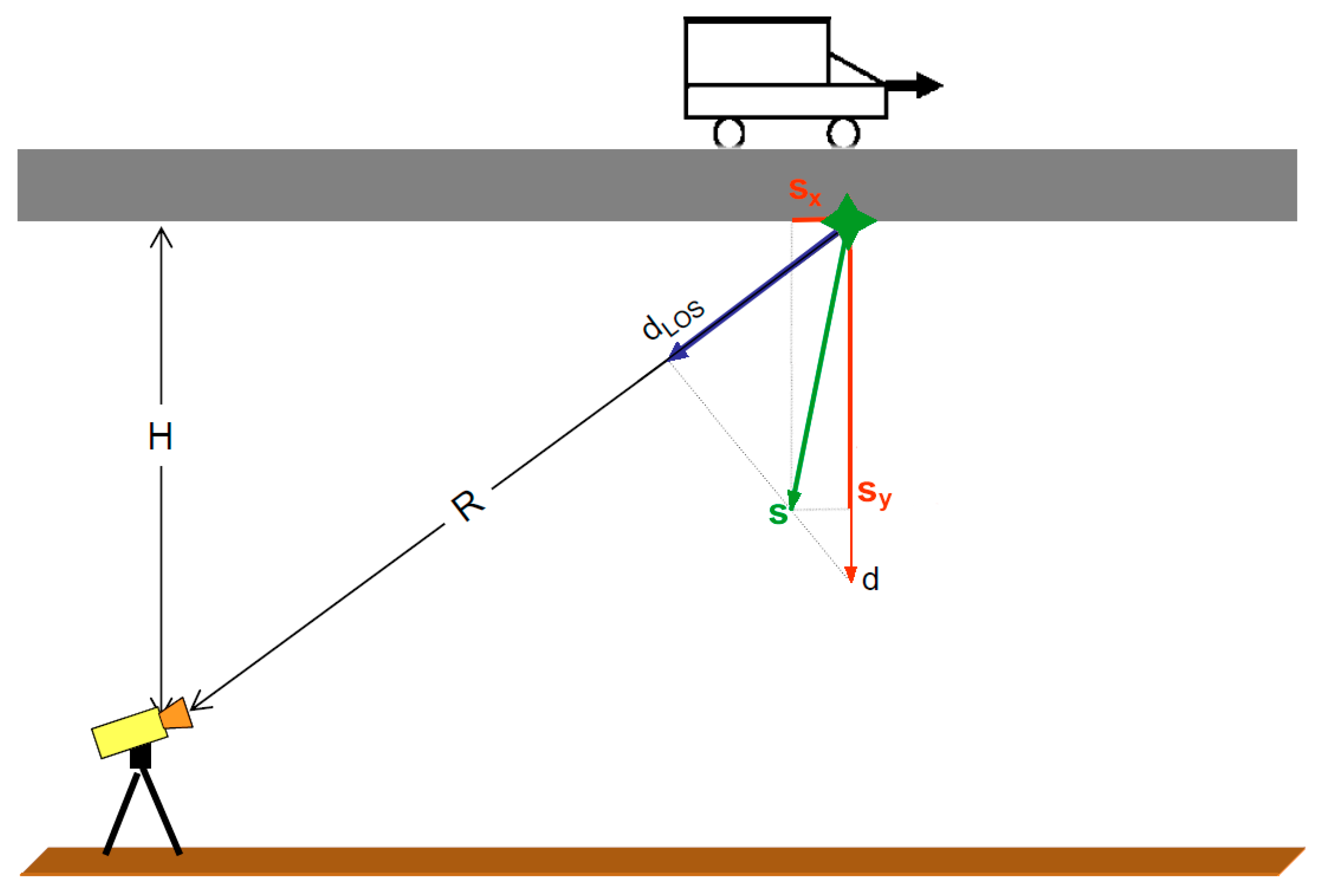
2.3. Accuracy Analysis of Longitudinal and Vertical Component of the Total Displacement
| … | covariance matrix of displacement vector s; | |
| … | covariance matrix of components of vector u; | |
| … | Jacobian matrix of mapping given by (9); | |
| … | vector of measured or approximately computed values of input quantities i.e., |
2.3.1. The Case When Imprecision of LOS Directions Is Neglected
| a | … | main axis size of the ellipse, |
| b | … | semi axis size of the ellipse, |
| φ | … | orientation of the main axis (in radians), |
| D | … | discriminant of the covariance matrix, |
| ind | … | dicator function, |
2.3.2. The Case When Imprecision of LOS Directions Is Considered
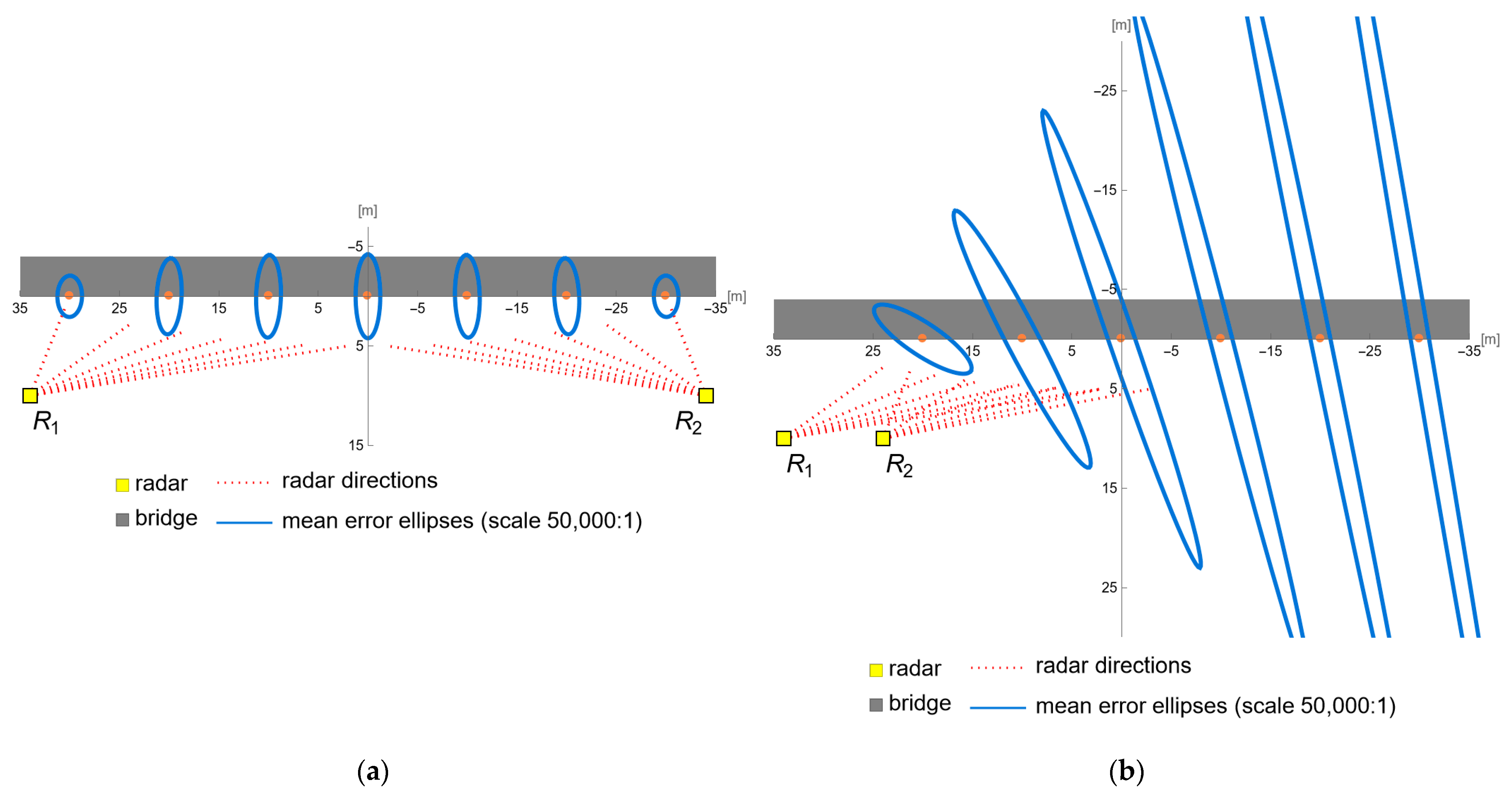
2.3.3. The Case of Placing Radars behind Each Other
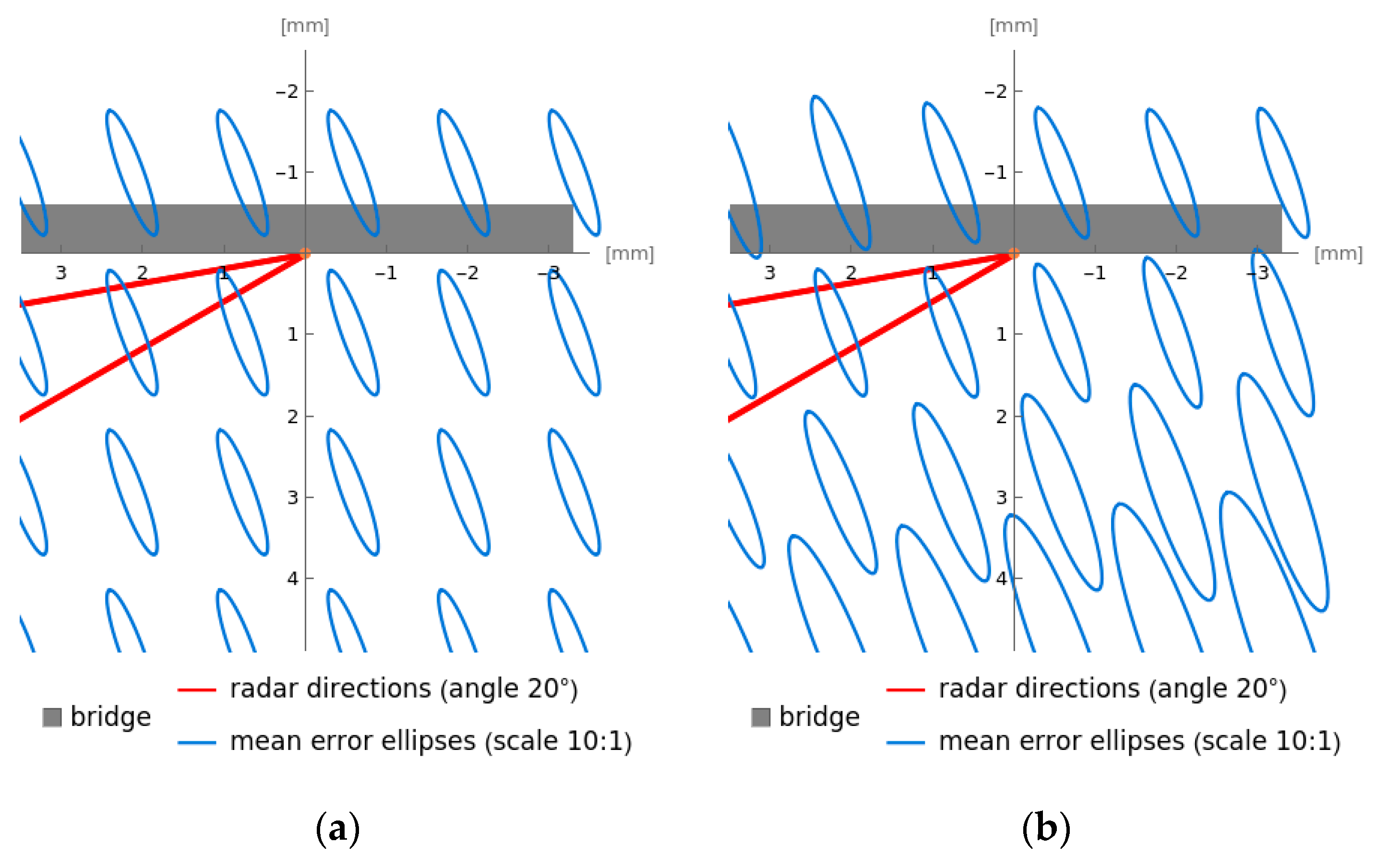
2.3.4. Accuracy Analysis in Different Locations of the Monitored Bridge
2.3.5. Accuracy Analysis Separately in Vertical and Longitudinal Directions
2.3.6. Summary of Accuracy Analysis Findings
- Imprecision of LOS directions is neglected—covariance matrix is given (Section 2.3.1).
- Precision of LOS directions is considered—covariance matrices , are given (Section 2.3.2).
2.4. Experimental Measurement in Order to Verify Theory
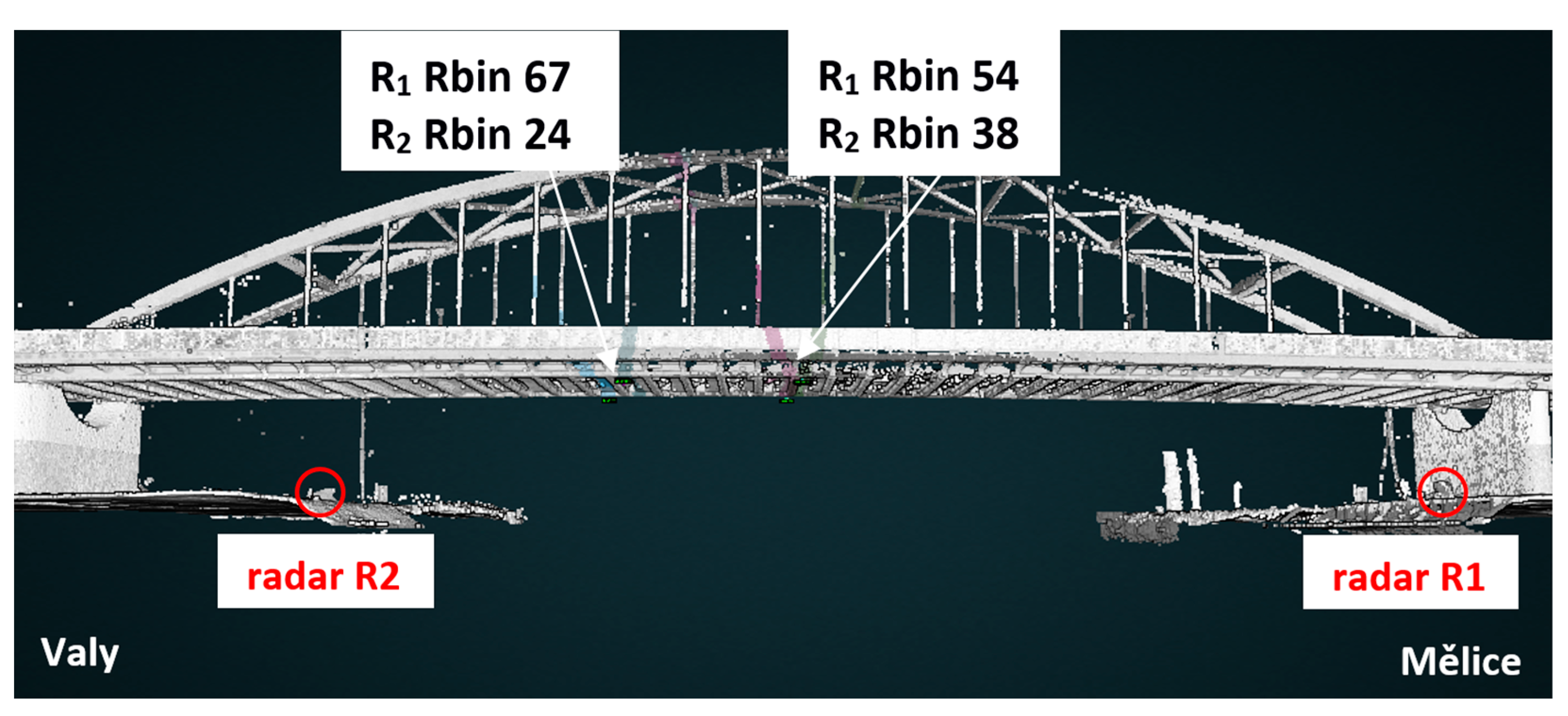
2.4.1. Experimental Measurement of the Arch Road Bridge “Valy”
Description of the Observed Bridge
Used Radar Interferometry Equipment
Used Standard Measuring Equipment
Measurement Configuration
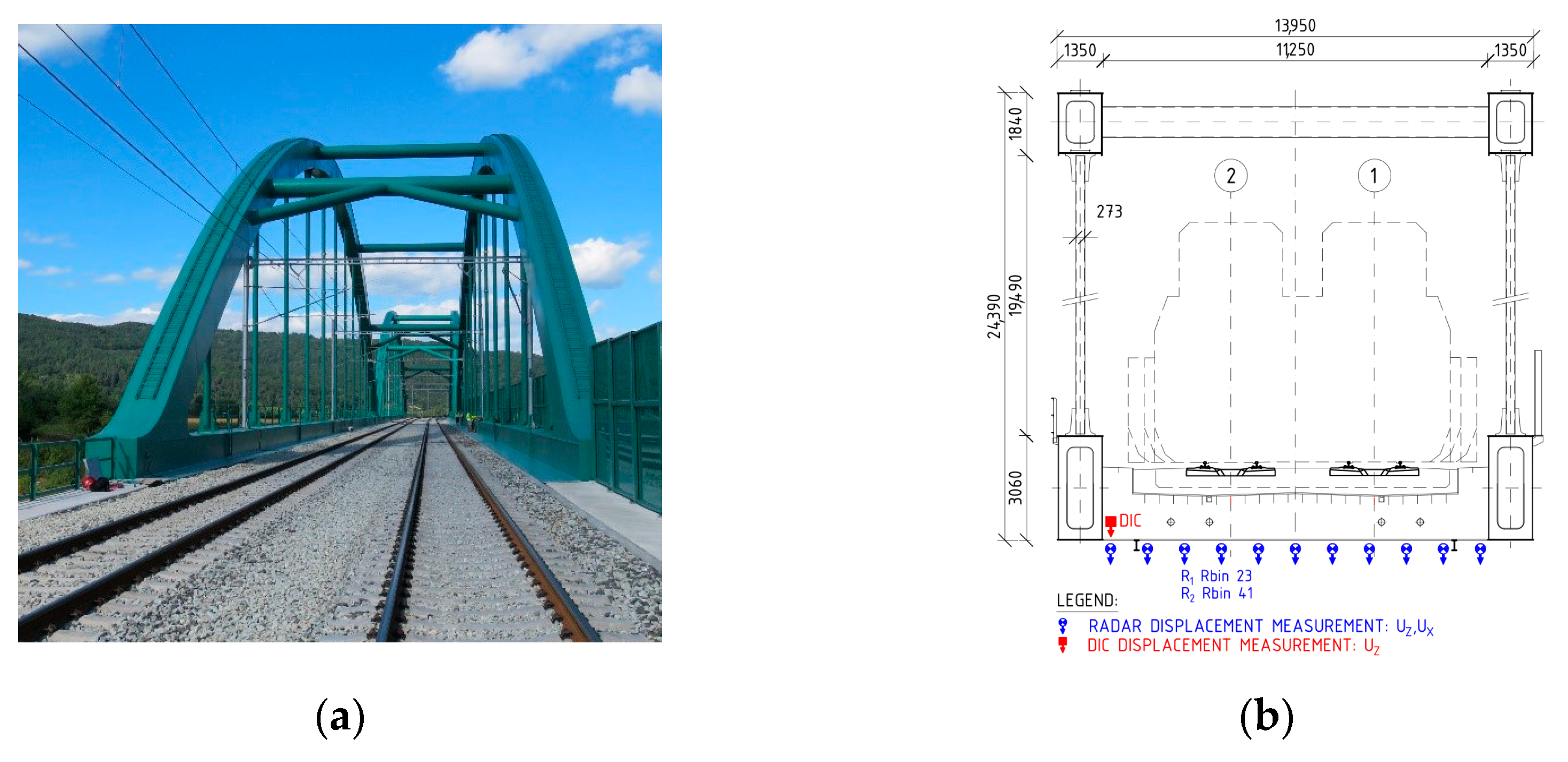
2.4.2. Experimental Measurement of the Railway Bridge “Púchov”
Description of the Observed Bridge
Used Standard Measuring Equipment
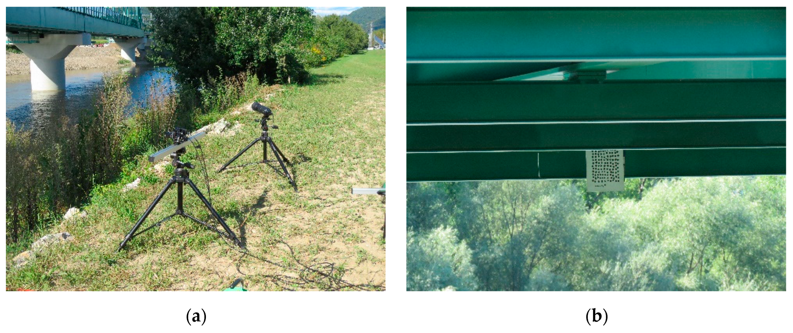
Used Radar Interferometry Equipment
Used Photogrammetric Digital Image Correlation Equipment
3. Results
3.1. Tests on the Bridge “Valy”
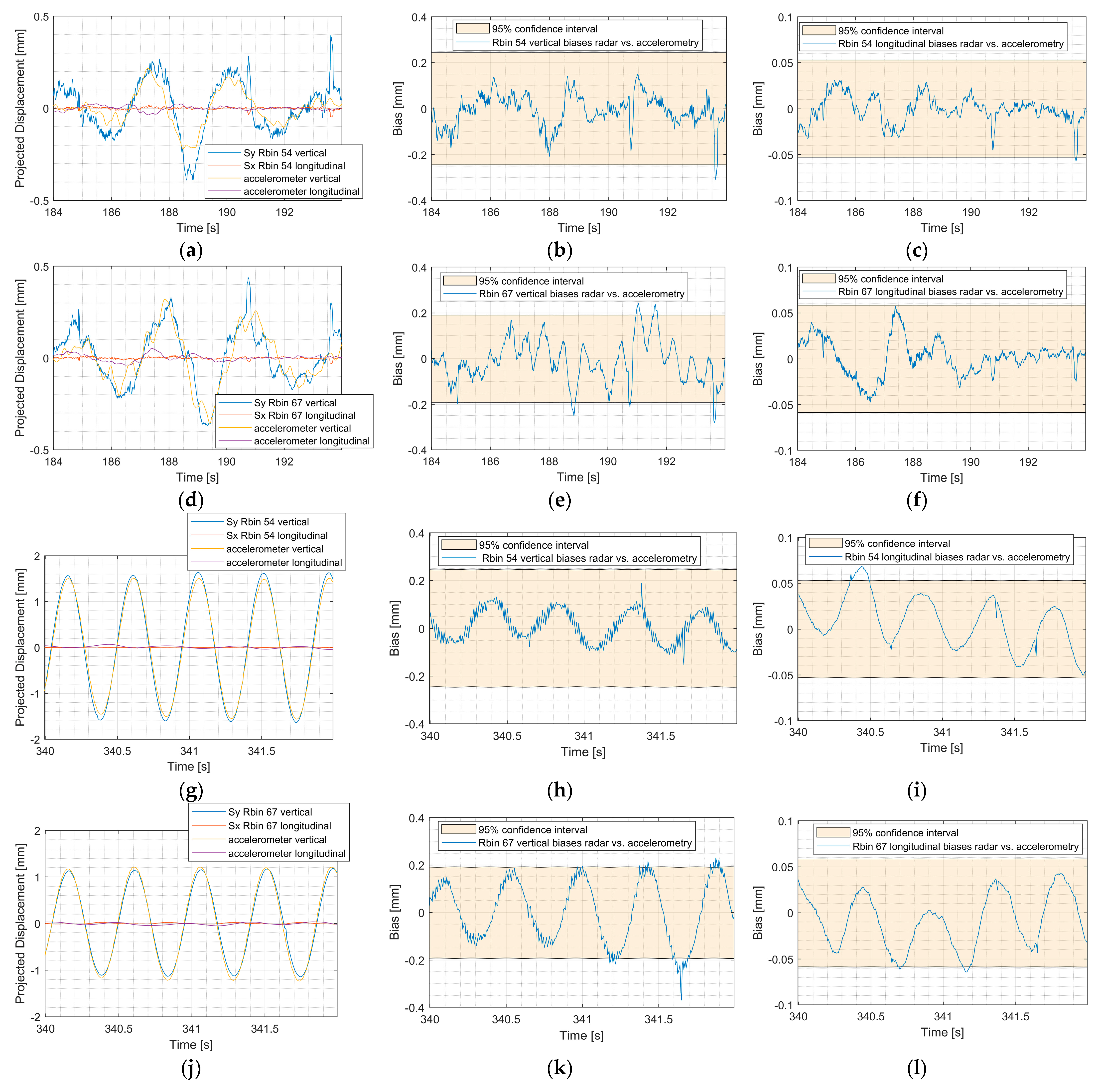
3.2. Tests on the Bridge “Púchov”
4. Discussion
5. Conclusions
- to highlight necessity of simultaneous usage of two interferometric radars to eliminate the Interpretation Error;
- to achieve the highest possible accuracy in determining the resulting total displacements.
- description of the current state and analysis of Interpretation Errors EI when measuring with single radar (see the Section 1);
- presentation of the principles of measurement by two radars with the accuracy analysis of the resulting displacements (see the Section 2.1, Section 2.2 and Section 2.3);
- verification of the results in practice by experimental measurement (see the Section 2.4 and Section 3);
Author Contributions
Funding
Data Availability Statement
Acknowledgments
Conflicts of Interest
References
- Sung, Y.-C.; Lin, T.-K.; Chiu, Y.-T.; Chang, K.-C.; Chen, K.-L.; Chang, C.-C. A bridge safety monitoring system for prestressed composite box-girder bridges with corrugated steel webs based on in-situ loading experiments and a long-term monitoring database. Eng. Struct. 2016, 126, 571–585. [Google Scholar] [CrossRef]
- Kašpárek, J.; Ryjáček, P.; Rotter, T.; Polák, M.; Calçada, R. Long-term monitoring of the track–bridge interaction on an extremely skew steel arch bridge. J. Civ. Struct. Health Monit. 2020, 10, 377–3871. [Google Scholar] [CrossRef]
- Pieraccini, M.; Fratini, M.; Parrini, F.; Atzeni, C. Dynamic Monitoring of Bridges Using a High-Speed Coherent Radar. IEEE Trans. Geosci. Remote Sens. 2006, 44, 3284–3288. [Google Scholar] [CrossRef]
- Pieraccini, M.; Parrini, F.; Fratini, M.; Atzeni, C.; Spinelli, P.; Micheloni, M. Static and Dynamic Testing of Bridges through Microwave Interferometry. NDT E Int. 2007, 40, 208–214. [Google Scholar] [CrossRef]
- Gentile, C.; Bernardini, G. Radar-Based Measurement of Deflections on Bridges and Large Structures. Eur. J. Environ. Civ. Eng. 2010, 14, 495–516. [Google Scholar] [CrossRef]
- Lipták, I.; Erdélyi, J.; Kyrinovič, P.; Kopáčik, A. Monitoring of Bridge Dynamics by Radar Interferometry. Geoinform. FCE CTU 2014, 12, 10–15. [Google Scholar] [CrossRef] [PubMed]
- Liu, X.; Tong, X.; Ding, K.; Zhao, X.; Zhu, L.; Zhang, X. Measurement of Long-Term Periodic and Dynamic Deflection of the Long-Span Railway Bridge Using Microwave Interferometry. IEEE J. Sel. Top. Appl. Earth Obs. Remote Sens. 2015, 8, 4531–4538. [Google Scholar] [CrossRef]
- Talich, M. The Effect of Temperature Changes on Vertical Deflections of Metal Rail Bridge Constructions Determined by the Ground Based Radar Interferometry Method. IOP Conf. Ser. Earth Environ. Sci. 2019, 221, 012076. [Google Scholar] [CrossRef]
- Luzi, G.; Crosetto, M.; Fernández, E. Radar Interferometry for Monitoring the Vibration Characteristics of Buildings and Civil Structures: Recent Case Studies in Spain. Sensors 2017, 17, 669. [Google Scholar] [CrossRef]
- Talich, M. Monitoring of horizontal movements of high-rise buildings and tower transmitters by means of ground-based interferometric radar. Int. Arch. Photogramm. Remote Sens. Spatial Inf. Sci. 2018, 42, 499–504. [Google Scholar] [CrossRef]
- Talich, M. Using Ground Radar Interferometry for Precise Determining of Deformation and Vertical Deflection of Structures. IOP Conf. Ser. Earth Environ. Sci. 2017, 95, 032021. [Google Scholar] [CrossRef]
- Artese, S.; Nico, G. TLS and GB-RAR Measurements of Vibration Frequencies and Oscillation Amplitudes of Tall Structures: An Application to Wind Towers. Appl. Sci. 2020, 10, 2237. [Google Scholar] [CrossRef]
- Pieraccini, M.; Fratini, M.; Parrini, F.; Atzeni, C.; Bartoli, G. Interferometric Radar vs. Accelerometer for Dynamic Monitoring of Large Structures: An Experimental Comparison. NDT E Int. 2008, 41, 258–264. [Google Scholar] [CrossRef]
- Akbar, S.J. Dynamic monitoring of bridges: Accelerometer Vs microwave radar interferometry (IBIS-S). J. Phys. Conf. Ser. 2021, 1882, 012124. [Google Scholar]
- Yu, J.; Meng, X.; Yan, B.; Xu, B.; Fan, Q.; Xie, Y. Global Navigation Satellite System-based positioning technology for structural health monitoring: A review. Struct. Control Health Monit. 2020, 27, e2467. [Google Scholar] [CrossRef]
- Liu, X.; Wang, P.; Lu, Z.; Gao, K.; Wang, H.; Jiao, C.; Zhang, X. Damage Detection and Analysis of Urban Bridges Using Terrestrial Laser Scanning (TLS), Ground-Based Microwave Interferometry, and Permanent Scatterer Interferometry Synthetic Aperture Radar (PS-InSAR). Remote Sens. 2019, 11, 580. [Google Scholar] [CrossRef]
- Rashidi, M.; Mohammadi, M.; Sadeghlou Kivi, S.; Abdolvand, M.M.; Truong-Hong, L.; Samali, B. A Decade of Modern Bridge Monitoring Using Terrestrial Laser Scanning: Review and Future Directions. Remote Sens. 2020, 12, 3796. [Google Scholar] [CrossRef]
- Nettis, A.; Massimi, V.; Nutricato, R.; Nitti, D.O.; Samarelli, S.; Uva, G. Satellite-based interferometry for monitoring structural deformations of bridge portfolios. Autom. Constr. 2023, 147, 104707. [Google Scholar] [CrossRef]
- Lee, Z.-K.; Bonopera, M.; Hsu, C.-C.; Lee, B.-H.; Yeh, F.-Y. Long-term deflection monitoring of a box girder bridge with an optical-fiber, liquid-level system. Structures 2022, 44, 904–919. [Google Scholar] [CrossRef]
- Gentile, C.; Bernardini, G. An Interferometric Radar for Non-Contact Measurement of Deflections on Civil Engineering Structures: Laboratory and Full-Scale Tests. Struct. Infrastruct. Eng. 2010, 6, 521–534. [Google Scholar] [CrossRef]
- Xiang, J.; Zeng, Q.; Lou, P. Transverse Vibration of Train-Bridge and Train-Track Time Varying System and the Theory of Random Energy Analysis for Train Derailment. Veh. Syst. Dyn. 2004, 41, 129–155. [Google Scholar] [CrossRef]
- Jin, Z.; Pei, S.; Li, X.; Qiang, S. Vehicle-Induced Lateral Vibration of Railway Bridges: An Analytical-Solution Approach. J. Bridge Eng. 2016, 21, 04015038. [Google Scholar] [CrossRef]
- Miccinesi, L.; Beni, A.; Pieraccini, M. Multi-Monostatic Interferometric Radar for Bridge Monitoring. Electronics 2021, 10, 247. [Google Scholar] [CrossRef]
- Olaszek, P.; Świercz, A.; Boscagli, F. The Integration of Two Interferometric Radars for Measuring Dynamic Displacement of Bridges. Remote Sens. 2021, 13, 3668. [Google Scholar] [CrossRef]
- Dei, D.; Mecatti, D.; Pieraccini, M. Static Testing of a Bridge Using an Interferometric Radar: The Case Study of “Ponte Degli Alpini”, Belluno, Italy. Sci. World J. 2013, 2013, e504958. [Google Scholar] [CrossRef] [PubMed]
- IDS Ingegneria Dei Sistemi, S.p.A. Static and Dynamic Testing of Bridges: Use of IBIS-FS for Measuring Deformation and Identifying Modal Analysis Parameters; IDS: Pisa, Italy, 2016; p. 56. [Google Scholar]
- Monti-Guarnieri, A.; Falcone, P.; D’Aria, D.; Giunta, G. 3D Vibration Estimation from Ground-Based Radar. Remote Sens. 2018, 10, 1670. [Google Scholar] [CrossRef]
- Michel, C.; Keller, S. Advancing Ground-Based Radar Processing for Bridge Infrastructure Monitoring. Sensors 2021, 21, 2172. [Google Scholar] [CrossRef]
- Miccinesi, L.; Pieraccini, M. Bridge Monitoring by a Monostatic/Bistatic Interferometric Radar Able to Retrieve the Dynamic 3D Displacement Vector. IEEE Access 2020, 8, 210339–210346. [Google Scholar] [CrossRef]
- Mills, D.; Martin, J.; Burbank, J.; Kasch, W. Network Time Protocol Version 4: Protocol and Algorithms Specification, RFC 5905. 2010. Available online: https://www.rfc-editor.org/info/rfc5905 (accessed on 27 December 2022).
- Windows Time Service Technical Reference. Available online: https://learn.microsoft.com/en-us/windows-server/networking/windows-time-service/windows-time-service-tech-ref (accessed on 1 December 2022).
- Rao, C.R. Linear Statistical Inference and Its Applications, 2nd ed.; Wiley: New York, NY, USA, 2009; p. 519. [Google Scholar]
- Perry, B.J.; Guo, Y.; Atadero, R.; van de Lindt, J.W. Unmanned aerial vehicle (UAV)-enabled bridge inspection framework. In Bridge Maintenance, Safety, Management, Life-Cycle Sustainability and Innovations; Yokota, H., Frangopol, D.M., Eds.; Taylor & Francis Group: London, UK, 2021; pp. 158–165. [Google Scholar]
- Wang, F.; Zou, Y.; del Rey Castillo, E.; Ding, Y.; Xu, Z.; Zhao, H.; James, B.P. Lim Automated UAV path-planning for high-quality photogrammetric 3D bridge reconstruction. Struct. Infrastruct. Eng. 2022, 1–20. [Google Scholar]
- Simpson’s Rule. Available online: https://en.wikipedia.org/wiki/Simpson%27s_rule (accessed on 26 December 2022).
- Oppenheim, A.V.; Schafer, R.W.; Buck, J.R. Discrete-Time Signal Processing, 2nd ed.; Prentice Hall: Upper Saddle River, NJ, USA, 1999; p. 896. ISBN 0-13-754920-2. [Google Scholar]


| R/H\sx/sy | 0.01 | 0.04 | 0.07 | 0.10 | 0.15 | 0.20 | 0.25 | 0.30 | 0.40 | 0.50 |
|---|---|---|---|---|---|---|---|---|---|---|
| 1.00 | 0% | 0% | 0% | 0% | 0% | 0% | 0% | 0% | 0% | 0% |
| 1.20 | 1% | 3% | 5% | 7% | 10% | 13% | 17% | 20% | 27% | 33% |
| 1.40 | 1% | 4% | 7% | 10% | 15% | 20% | 24% | 29% | 39% | 49% |
| 1.60 | 1% | 5% | 9% | 12% | 19% | 25% | 31% | 37% | 50% | 62% |
| 1.80 | 1% | 6% | 10% | 15% | 22% | 30% | 37% | 45% | 60% | 75% |
| 2.00 | 2% | 7% | 12% | 17% | 26% | 35% | 43% | 52% | 69% | 87% |
| 2.50 | 2% | 9% | 16% | 23% | 34% | 46% | 57% | 69% | 92% | 115% |
| 3.00 | 3% | 11% | 20% | 28% | 42% | 57% | 71% | 85% | 113% | 141% |
| 3.50 | 3% | 13% | 23% | 34% | 50% | 67% | 84% | 101% | 134% | 168% |
| 4.00 | 4% | 15% | 27% | 39% | 58% | 77% | 97% | 116% | 155% | 194% |
| 4.50 | 4% | 18% | 31% | 44% | 66% | 88% | 110% | 132% | 175% | 219% |
| 5.00 | 5% | 20% | 34% | 49% | 73% | 98% | 122% | 147% | 196% | 245% |
| 5.50 | 5% | 22% | 38% | 54% | 81% | 108% | 135% | 162% | 216% | 270% |
| 6.00 | 6% | 24% | 41% | 59% | 89% | 118% | 148% | 177% | 237% | 296% |
| 7.00 | 7% | 28% | 48% | 69% | 104% | 139% | 173% | 208% | 277% | 346% |
| 8.00 | 8% | 32% | 56% | 79% | 119% | 159% | 198% | 238% | 317% | 397% |
| 9.00 | 9% | 36% | 63% | 89% | 134% | 179% | 224% | 268% | 358% | 447% |
| 10.00 | 10% | 40% | 70% | 99% | 149% | 199% | 249% | 298% | 398% | 497% |
| Case | Substitutions | |
|---|---|---|
| LOS imprecision neglected | (14), (13) | |
| LOS precision considered | (12), (10), (16), (13), (17) |
| R1: Radar IBIS—FS Plus | R2: Radar IBIS—RU 172 | |
|---|---|---|
| Sampling frequency | 200 Hz | 199.2 Hz 1 |
| Signal range (max. distance) | 75 m | 70 m |
| Rbin (range resolution area) | 0.75 m | 0.75 m |
| R1: Radar IBIS—FS Plus | R2: Radar IBIS—RU 172 | |
|---|---|---|
| Sampling frequency | 200 Hz | 199.2 Hz 1 |
| Signal range (max. distance) | 100 m | 120 m |
| Rbin (range resolution area) | 0.75 m | 0.75 m |
| Vertical tilt of the radar | 0.0° | 53.9° 1 |
Disclaimer/Publisher’s Note: The statements, opinions and data contained in all publications are solely those of the individual author(s) and contributor(s) and not of MDPI and/or the editor(s). MDPI and/or the editor(s) disclaim responsibility for any injury to people or property resulting from any ideas, methods, instructions or products referred to in the content. |
© 2023 by the authors. Licensee MDPI, Basel, Switzerland. This article is an open access article distributed under the terms and conditions of the Creative Commons Attribution (CC BY) license (https://creativecommons.org/licenses/by/4.0/).
Share and Cite
Talich, M.; Havrlant, J.; Soukup, L.; Plachý, T.; Polák, M.; Antoš, F.; Ryjáček, P.; Stančík, V. Accuracy Analysis and Appropriate Strategy for Determining Dynamic and Quasi-Static Bridge Structural Response Using Simultaneous Measurements with Two Real Aperture Ground-Based Radars. Remote Sens. 2023, 15, 837. https://doi.org/10.3390/rs15030837
Talich M, Havrlant J, Soukup L, Plachý T, Polák M, Antoš F, Ryjáček P, Stančík V. Accuracy Analysis and Appropriate Strategy for Determining Dynamic and Quasi-Static Bridge Structural Response Using Simultaneous Measurements with Two Real Aperture Ground-Based Radars. Remote Sensing. 2023; 15(3):837. https://doi.org/10.3390/rs15030837
Chicago/Turabian StyleTalich, Milan, Jan Havrlant, Lubomír Soukup, Tomáš Plachý, Michal Polák, Filip Antoš, Pavel Ryjáček, and Vojtěch Stančík. 2023. "Accuracy Analysis and Appropriate Strategy for Determining Dynamic and Quasi-Static Bridge Structural Response Using Simultaneous Measurements with Two Real Aperture Ground-Based Radars" Remote Sensing 15, no. 3: 837. https://doi.org/10.3390/rs15030837
APA StyleTalich, M., Havrlant, J., Soukup, L., Plachý, T., Polák, M., Antoš, F., Ryjáček, P., & Stančík, V. (2023). Accuracy Analysis and Appropriate Strategy for Determining Dynamic and Quasi-Static Bridge Structural Response Using Simultaneous Measurements with Two Real Aperture Ground-Based Radars. Remote Sensing, 15(3), 837. https://doi.org/10.3390/rs15030837