Electromagnetic Scattering and Doppler Spectrum Simulation of Land–Sea Junction Composite Rough Surface

Abstract

In this paper, a weighted arctangent function is used in conjunction with the spectral method to generate a land–sea junction composite rough surface under the spatially homogeneous and time-stationary hypotheses. The exponential correlation function and the Joint North Sea Wave Project (JONSWAP) spectrum, combined with an experiment-verified shoaling coefficient, are applied to model the land surfaces and the time-varying sea surfaces separately. The second-order small slope approximation (SSA-II) with tapered wave incidence is utilized for evaluating the electromagnetic scattering characteristics and Doppler characteristics of the generated composite rough surface. The influence of land–sea interface factors on radar cross-section (RCS) and Doppler shift of radar echoes is investigated in detail by comparing the RCS and Doppler spectra of the land–sea junction composite rough surfaces with those of finite-depth sea surfaces. It can be found that the Doppler spectra of the land–sea junction composite rough surface is narrower than that of the finite-depth sea surface under upwind directions and wider than that of the finite-depth sea surface under crosswind directions.

1. Introduction

With the development of computational electromagnetic (CEM), the electromagnetic (EM) scattering characteristics and Doppler characteristics of random rough surface have received a great deal of attention in recent years from a range of applications, such as radar imaging, surface remote sensing, and ocean wave spectra estimation. Thus far, several methods have been proposed to evaluate the EM scattering from a rough surface. For example, the method of moments (MoM) combined with Rao–Wilton–Glisson (RWG) basis functions and Poggio–Miller–Chang–Harrington–Wu (PMCHW) integral equations is proposed and utilized to solve EM scattering from a rough surface in [1]. The multilevel fast multipole algorithm (MLFMA), together with the impedance boundary conditions (IBC) and the self-dual integral equation, is applied to calculate the backscattering from a rough sea surface under low grazing incidence [2]. A stochastic solution of the EM scattering from a penetrable, randomly rough surface is derived by using the vector-based-finite-element method (FEM) in [3]. Li et al. combined the Finite-Difference Time-Domain (FDTD) approach with the uniaxial perfectly matched layer (UPML) absorbing boundary to solve the EM scattering problems of 1-D rough sea surfaces [4], 2-D rough sea surfaces [5], and two-layered rough surfaces [6]. The time domain integral equation (TDIE) is applied to simulate the transient scattering from the ocean surface with ship wake in [7]. In [8], a second stochastic degree iterative algorithm with sparse matrix (SM) and Chebyshev approximation is proposed to calculate the fully polarimetric bistatic scattering behavior that resulted from the interaction of an EM wave with all scales of ocean waves. Saddek Afifi uses the first-order small slope approximation (SSA-I) and the first-order small perturbation method (SPM-I) to study the EM scattering from a 2-D random rough surface that separates the vacuum from a perfect electromagnetic conductor (PEMC) [9]. The second-order small slope approximation (SSA-II) is applied to solve the bis- and mono-static scattering from linear and non-linear rough sea surfaces in [10,11,12]. The second-order small perturbation method (SPM-II) is applied to solve the EM scattering from layered mediums with rough interfaces by Hasan Zamani [13,14] and R. J. Burkholder [15]. A semi-deterministic facet model (SDFM) is proposed in [16] to simulate the EM scattering from an ocean-like surface. In [17], the advanced integral equation model (AIEM) is applied to predict the backscattering, bistatic scattering, and emission of rough soil surfaces. Wang and Tong proposed an improved facet-based model derived from a two-scale model (TSM) to evaluate the scattering strength of an electrically large ocean surface [18]. In [19,20,21,22,23], the first-order SSA and TSM models are utilized to solve monostatic and bistatic scattering from randomly rough surfaces (sea surface covered with or without oil film, ground surface) in different frequency bands.

However, in all of the literature mentioned above, the processed rough surface is the sea surface or ground surface, which contains only one type of background surface and one power spectrum. It is possible that both the sea surface and ground surface exist in one beam in the real radar detection. Due to the difference in the dielectric parameters and the surface profile between the land–sea junction composite rough surface and the sea (ground) surface, the EM scattering characteristics of the land–sea junction composite rough surface are correspondingly different from those of the sea surface and those of the ground surface. Motivated by the reasons illustrated above, our focus in this paper is on the influence of land–sea interface factors on radar cross-section (RCS) and Doppler spectra of EM scattered echoes of the land–sea junction composite rough surface, which has a frozen land surface and a time-evolving sea surface. The research in this paper is potentially valuable for remote sensing, target detection in land–sea junction areas, etc. Due to desirable properties such as analytical tractability and numerical efficiency, in this paper the nonlinear hydrodynamic model of the JONSWAP spectrum combined with an experiment-verified shoaling coefficient is used to model a finite-depth sea surface, and the exponential correlation function is adopted to model the ground surface. A weighted arctangent function is introduced to smoothly connect the sea surface and the ground surface, and to model the land–sea junction composite rough surface. Compared with the classical models such as Kirchhoff approximation (KA), TSM, and SPM, SSA-II takes into account facets’ tilt modulation and second-order Bragg scattering and is thus capable of reasonably predicting the RCS and Doppler spectra. Therefore, the SSA-II is employed to evaluate the RCS and Doppler spectra of radar echoes from sea surfaces and land–sea junction composite rough surfaces in this study.

In [24,25,26,27,28], several methods have been proposed to solve electromagnetic scattering from a land–sea junction composite rough surface or a target located above a coastal environment. This paper has advantages over the literature cited previously. First, the SSA-II is applied as the electromagnetic scattering kernel since it is more accurate than the techniques in the aforementioned literature and can account for second-order Bragg scattering. Second, this paper focuses on the analysis of Doppler characteristics of the land–sea junction composite rough surface, which is not involved in the prior literature. The weighted arctangent function was originally introduced in [29] to generate a land–sea junction composite rough surface, but there are several differences between [29] and this paper. First, although the weighted arctangent function has been introduced both in [29] and the manuscript under review, the two functions have different forms. Second, the Modified Equivalent Current Approximation (MECA) is used to calculate the EM scattering fields from the composite rough surface in [29], which can only take into account the specular reflection effect. In this paper, the SSA-II is applied as the electromagnetic scattering kernel, which is more accurate than MECA and can take into account second-order Bragg scattering. Third, the EM scattering from a target located in the land–sea junction area is the primary issue addressed in [29]. In this paper, the RCS and Doppler spectra of the land–sea junction composite rough surface are calculated and discussed in detail.

The remainder of this paper is organized as follows: in Section 2, the weighted arctangent function is introduced, and the modeling of the land–sea junction composite rough surface is presented. Section 3 presents the SSA-II EM scattering model with tapered wave incidence for evaluating the RCS of rough surfaces (sea surface and land–sea junction composite rough surface). A comparison of the numerical results of the RCS and Doppler spectra for finite-depth sea surface and land–sea junction composite rough surfaces is presented and discussed in Section 4. Section 5 is devoted to the conclusions of this paper.

2. Modeling of Land–Sea Junction Composite Surface

2.1. Sea Spectrum of Finite-Depth Sea Water

With the change of the water depth and seabed topography, the profile and the statistical characteristics of the sea surface in coastal areas are different from those in deep sea areas. In [30], a shoaling coefficient is proposed by McCormick to study the effect of water depth on the wave height, which can be written as

$$\varsigma (d)=\sqrt{\frac{{\cosh }^2(kd)}{\sinh (kd)\cosh (kd)+kd}}$$

(1)

in which $d$ and $k$ represent the depth and the wave number of the sea surface, respectively.

According to McCormick’s theory, the spectrum of actively growing wind waves in finite-depth seas can be analytically expressed as

$${S^{\prime }}_{\mathrm{finite}}(\omega )=S_{\mathrm{JONSWAP}}(\omega ){\varsigma }^2(d)$$

(2)

$$S_{\mathrm{finite}}(k)={S^{\prime }}_{\mathrm{finite}}(\omega )\frac{\partial \omega }{\partial k}{\varsigma }^2(d)$$

(3)

where ${S^{\prime }}_{\mathrm{finite}}(\omega )$ and $S_{\mathrm{finite}}(k)$ are the spectrums of finite-depth seas. $S_{\mathrm{JONSWAP}}(\omega )$ denotes the JONSWAP spectrum, $\omega$ is the angular frequency of sea waves, which can be related according to the shallow water gravity capillarity dispersion relation as

$$\omega =\sqrt{g_{0}k(1+k^2/k_m^2)\tanh (kd)}$$

(4)

where $g_0$ is the acceleration of gravity and $k_m=363.2\mathrm{rad}/\mathrm{m}$ represents the wave number with minimum phase speed.

Figure 1 depicts the influence of water depth on the finite-depth sea spectrum. In Figure 1, the wind fetch involved in the finite-depth sea spectrum is set to 50 km, and the wind speed at 10 m height is set to $u_{10}=10 \mathrm{m}/\mathrm{s}$. It can be seen from Figure 1a that the peak value of the curves first decreases and then increases as the water depth decreases. Furthermore, it is evident that the peaks of angular frequency $\omega$ remain unchanged with the decrease of water depth, whereas the peaks of wave number $k$ shift toward the high-frequency part as the water depth decreases.

2.2. Rough Surface Realizations

To analyze the radar echoes (RCS, Doppler spectra), the geometric properties of the land–sea junction composite rough surface must be captured. In this paper, the spectral method under the spatially homogeneous and time-stationary hypothesis is applied to yield the rough finite-depth sea surface and ground surface, which is highly efficient due to the introduction of the fast Fourier transform. To establish a rough surface with the spectral method, a linear superposition of harmonic waves whose amplitudes are independent, normally distributed random values times the square root of the sea/ground surface spatial spectrum is generated, and the Fourier amplitude at any time $t$ can be expressed as

$$\begin{array}{c}A(k,t)=\gamma (k)\sqrt{S(k,\phi )\delta k_x\delta k_y}\exp (i\omega t)\\ +\gamma (-\mathit{k}{)}^{\ast }\sqrt{S(k,\pi -\phi )\delta k_x\delta k_y}\exp (-i\omega t)\end{array}$$

(5)

where $\mathit{k}$ is the two-dimensional spatial wave vector, $S(k,\phi )$ is the two-dimensional sea/ground spectrum (for the finite-depth sea surface, Elfouhaily wind direction function is applied), and $\delta k_x=2\pi /L_x$ and $\delta k_y=2\pi /L_y$ represent the sampling interval along x and y directions, respectively. $\gamma (\mathit{k})$ is a complex Gaussian series with zero mean and unit standard deviation.

Thus, the sea/ground surface elevation $h(\mathit{r},t)$ at position $\mathit{r}=(x,y)$ and time $t$ can be expressed by

$$h(\mathit{r},t)={\displaystyle \sum _{k}A(\mathit{k},t)\exp (i\mathit{k}·\mathit{r})}$$

(6)

Equation (6) can be efficiently accomplished by introducing the inverse fast Fourier transform. To ensure that $h(\mathit{r},t)$ is real, $A(\mathit{k},t)$ is required to satisfy the conjugate symmetry (Hermitian form) as follows:

$$A(k_x,k_y)=A^{\ast }(-k_x,-k_y)A(-k_x,k_y)=A^{\ast }(k_x,-k_y)$$

Figure 2 shows the simulated finite-depth sea surface under different water depths at a wind speed of $u_{10}=10 \mathrm{m}/\mathrm{s}$. It can be found that as the water depth decreases, the major sea wavelength decreases and, as a result, the major spatial wave number shifts to a high frequency, which is similar to that in Figure 1.

The exponential correlation function is utilized in the ground surface modeling for the realization of the land–sea junction composite rough surface.

2.3. Land–Sea Junction Composite Rough Surface Realizations

Once the finite-depth sea surface and the ground surface are generated, the only problem in realizing land–sea junction composite rough surface is how to smoothly connect the two rough surfaces with different undulations. The problem is solved in this study by introducing a weighted arctangent function, which can be described as:

$$f_{com}\left(x,y\right)={\omega }_1{f}_{sea}\left(x,y\right)+{\omega }_2{f}_{gro}\left(x,y\right)$$

(7)

in which $f_{com}\left(x,y\right)$ represents the land–sea junction composite rough surface, $f_{gro}\left(x,y\right)$ and $f_{sea}\left(x,y\right)$ are the ground surface and finite-depth sea surface, respectively. The weighted factors ${\omega }_1$ and ${\omega }_2$ can be written as ${\omega }_1=\left[\pi /2-\arctan (y-y_b)\right]/\pi$ and ${\omega }_2=\left[\pi /2+\arctan (y-y_b)\right]/\pi$, where $y_b$ is the boundary between the ground surface and the sea surface.

Figure 3 is a simple example of how the weighted arctangent function works. In Figure 3, the weighted arctangent function shown in Equation (7) is applied to smoothly connect the two flat plates (z = 0.1 for $y<0$ area, z = 0.5 for $y>0$ area). The area surrounding the boundary ($y=0$) of the two flat plates can be found to have continuous values and slopes.

The simulated land–sea junction composite rough surface obtained by introducing the weighted arctangent function is shown in Figure 4 and Figure 5. In Figure 4 and Figure 5, $y<0$ area is the finite-depth sea surface and the $y>0$ area is the ground surface. In the simulation, the length of the composite rough surface along the $x$- and $y$-axes is 256 m, and the wind speed and wind fetch are set as 5 m/s and 50 km, respectively. The water depth is 1 m. In Figure 4, the correlation length and root mean square height are $l_x=l_y=3.0 \mathrm{m}$ and $\delta =0.1 \mathrm{m}$. In Figure 5, the correlation length and root mean square height are $l_x=l_y=10.0 \mathrm{m}$ and $\delta =1.0 \mathrm{m}$. The wind direction in Figure 4a and Figure 5a is set as $\phi ={90}^{\circ }$, which means that the wind blew towards the shore. In Figure 4b and Figure 5b, the wind direction is set as $\phi =0^{\circ }$, which means that the wind blew along the coastline. The surface height and slope of the coastline area are continuous, as seen in Figure 4 and Figure 5.

3. SSA-II Model for EM Scattering from Land–Sea Junction Composite Rough Surface

The SSA proposed by Voronovich consists of a basic approximation of theory (SSA-I) and a second-order correction to it (SSA-II). The SSA-I only contains first-order Bragg scattering, which results in the fact that the SSA-I cannot predict the depolarization of wave scattering from a rough surface in the plane of incidence. Compared with other classical models (such as KA, TSM, and SPM), the SSA-II has its own advantages: (1) it takes into account the mutual transformation of the two linear polarization states caused by facets’ tilts; (2) it takes into account the second-order Bragg scattering and is thus capable of reasonably predicting the depolarized scattering from rough surfaces both in and outside the plane of incidence; and (3) a continuous spectrum of roughness is required, and it is not necessary to divide roughness into large- and small-scale components (just like it is in TSM). Due to the advantages mentioned above, the SSA-II model is used to evaluate the bistatic RCS, monostatic RCS, and Doppler spectra of the land–sea junction composite rough surface.

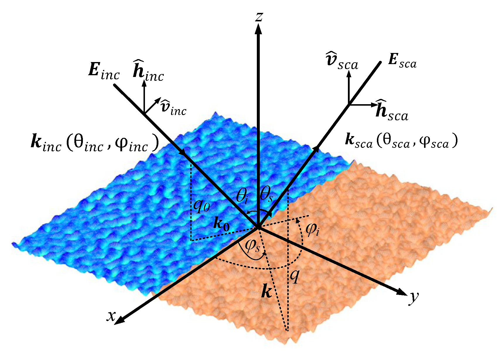
The SSA is based on the transformation properties of scattering amplitude (SA) with respect to vertical shifts. It claims that the slope of roughness is generally the only small parameter underlying this theory. Consider a tapered plane wave illuminated on a land–sea junction composite rough surface to reduce the edge effect caused by the limited surface size of $L_x\times L_y$, which can be expressed as

$${\mathit{E}}_{inc}(\mathit{r})=T(\mathit{r})\exp \left(i{\mathit{k}}_{inc}\cdot \mathit{r}\right)$$

(8)

$$T(\mathit{r})=\exp \left[i\left({\mathit{k}}_{inc}\cdot \mathit{r}\right)w\right]\exp \left(-t_x-t_y\right)$$

(9)

where

$$t_x=\frac{{\left(x\cos {\theta }_{inc}\cos {\phi }_{inc}+y\cos {\theta }_{inc}\sin {\phi }_{inc}+z\sin {\theta }_{inc}\right)}^2}{g^2{\cos }^2{\theta }_{inc}}$$

(10)

$$t_y=\frac{{\left(-x\sin {\phi }_{inc}+y\cos {\phi }_{inc}\right)}^2}{g^2}$$

(11)

$$w=\frac{1}{k_{inc}^2}\left(\frac{2t_x-1}{g^2{\cos }^2{\theta }_{inc}}+\frac{2t_y-1}{g^2}\right)$$

(12)

in which $g$ represents the tapered wave factor, which is set as $\max \{L_x,L_y\}/6$ in the following simulations. ${\theta }_{inc}$ and ${\phi }_{inc}$ denote the incident angle and incident azimuth angle, respectively.

The geometry of the scattering problem and corresponding notation are shown in Figure 6. ${\theta }_{sca}$ and ${\phi }_{sca}$ denote the scattering angle and scattering azimuth angle of the receiver, respectively. ${\mathit{k}}_{inc}={\mathit{k}}_0+q_0\widehat{z}$ and ${\mathit{k}}_{sca}={\mathit{k}}_1+q\widehat{z}$ are the incident wave vector and scattering wave vector, respectively; ${\mathit{k}}_0$ and ${\mathit{k}}_1$ denote the horizontal components of incident wave vector and scattering wave vector; and $q_0$ and $q$ are the vertical components of incident wave vector and scattering wave vector. $\widehat{h}$ and $\widehat{v}$ represent the polarizations of incident and scattering waves.

Thus, after introducing the tapered plane incident wave, the SA of the SSA-II model can be expressed as

$$\begin{array}{l}S\left({\mathit{k}}_1,{\mathit{k}}_0\right)=\frac{2\sqrt{q_{0}q}}{Q\sqrt{P_{inc}}}{\displaystyle \int \frac{d\mathit{r}T(\mathit{r})}{{\left(2\pi \right)}^2}}\exp \left(-i\left({\mathit{k}}_1-{\mathit{k}}_0\right)\cdot \mathit{r}+iQh\left(\mathit{r}\right)\right)\\ \times [B\left({\mathit{k}}_1,{\mathit{k}}_0\right)-\frac{i}{4}{\displaystyle \int M\left({\mathit{k}}_1,{\mathit{k}}_0;\xi \right)}h\left(\xi \right) \exp \left(i\xi \cdot \mathit{r}\right)\mathrm{d}\xi ]\end{array}$$

(13)

where

$$Q=q_0+q$$

$$h\left(\xi \right)=\frac{1}{{\left(2\pi \right)}^2}{\displaystyle \int h\left(\mathit{r}\right)\exp \left(-i\xi \cdot \mathit{r}\right)}d\mathit{r}$$

$h\left(\xi \right)$ represents the Fourier transform of the surface elevation. $P_{inc}$ denotes the incident wave power captured by the rough surface. The kernel functions $B$ and $M$ are $2\times 2$ matrices describing transitions of the EM waves of various polarizations into each other, which are mainly dependent on the configuration angles, polarizations, boundary conditions, and the permittivity of the lower medium. In fact, Bragg’s scattering is described by function $B$ in SSA, and the term relates to the function $M$ proportional to the slopes of a rough surface rather than to the elevations themselves. The corresponding details of these two kernel functions can be found in [31]. Thus, the average scattering coefficient can be expressed as

$$\sigma =4\pi q_0{q}_1〈{\left|S({\mathit{k}}_1,{\mathit{k}}_0)\right|}^2〉$$

(14)

where the angle brackets denote the ensemble average over random surface realizations. Furthermore, the Doppler spectrum can be defined as the power spectral density of the random time-varying scattering amplitude and can be evaluated by utilizing a standard spectral estimation technique by the following equation

$$S(f)=〈\frac{1}{T}{\left|{\displaystyle {\int }_0^{T}S\left({\mathit{k}}_1,{\mathit{k}}_0;t\right)e^{-i2\pi ft}dt}\right|}^2〉$$

(15)

where $S\left({\mathit{k}}_1,{\mathit{k}}_0;t\right)$ is the backscattering amplitude from rough surface at time $t$. It should be noted that when calculating the Doppler spectra of the land–sea junction composite rough surface, the sea surface is time-evolving, whereas the ground surface is constant and time-independent.

To quantitatively measure the Doppler spectrum, the Doppler shift $f_c$, that is, the spectral centroid, and the bandwidth of the Doppler spectrum $f_w$ can be defined as

$$f_c=\frac{{\displaystyle \int fS(f)df}}{{\displaystyle \int S}(f)df}$$

(16)

$$f_w=\sqrt{\frac{{\displaystyle \int {\left(f-f_c\right)}^{2}S(f)df}}{{\displaystyle \int S}(f)df}}$$

(17)

where $f_c$ represents the horizontal motion between ocean waves and observation radar, which can be used to invert the propulsion velocity of ocean waves. $f_w$ is mainly caused by the up-and-down motion of the points on the sea surface profile.

4. Numerical Results and Discussion

To validate SSA-II, a comparison of monostatic scattering coefficients of the sea surface derived from SSA-II with those from 3 months of Seasat microwave scatterometer (SASS) measurements [32] is performed and shown in Figure 7 under wind speed $u_{10}=5 \mathrm{m}/\mathrm{s}$ and $u_{10}=10 \mathrm{m}/\mathrm{s}$ for Ku-band (14.6 GHz) to validate SSA-II. According to the Debye expression [33], the relative permittivity of sea water is ${\epsilon }_r^{sea}=44.78+i39.12$ at sea water temperature of 20 °C and a salinity of 30 parts per thousand. The sampling interval is $\lambda /8$, where $\lambda$ is electromagnetic wavelength. The size of the sea surface is $L_x=L_y=10000\lambda$. The wind fetch is 100 km and 300 km. The wind direction is set as $\phi =0^{\circ }$, and the tapered incident wave is illuminated upwind to the sea surface with tapering parameter $g=\lambda /6$. The final monostatic scattering coefficient is an ensemble average of 50 realizations of sea surface.

It can be seen in Figure 7 that SSA-II is very consistent with the experimental data for both HH and VV polarizations. Additionally, the VV polarization has more accurate results than that of the HH polarization, especially at $u_{10}=10 \mathrm{m}/\mathrm{s}$. It is because the nonlinear effect of the sea surface is more obvious under HH polarization.

In the following, numerical simulations are performed at a frequency of $f=1.2\mathrm{GHz}$. The relative permittivity of sea surface and ground surface are ${\epsilon }_r^{sea}=73.2+i67.2$ and ${\epsilon }_r^{gro}=4.54+i0.36$, respectively. The length of three types of rough surfaces (sea surface, ground surface, and land–sea junction composite rough surface) is $L_x=L_y=128\lambda$, with sampling interval of $\lambda /8$. The tapering parament is set to be $g=\lambda /6$. The water depth and wind fetch are fixed at 5 m and 30 km, respectively. For the ground surface, the correlation length and root mean square height are $l_x=l_y=3.0 \mathrm{m}$ and $\delta =0.1 \mathrm{m}$, respectively. All numerical results are derived by averaging 50 surface realizations.

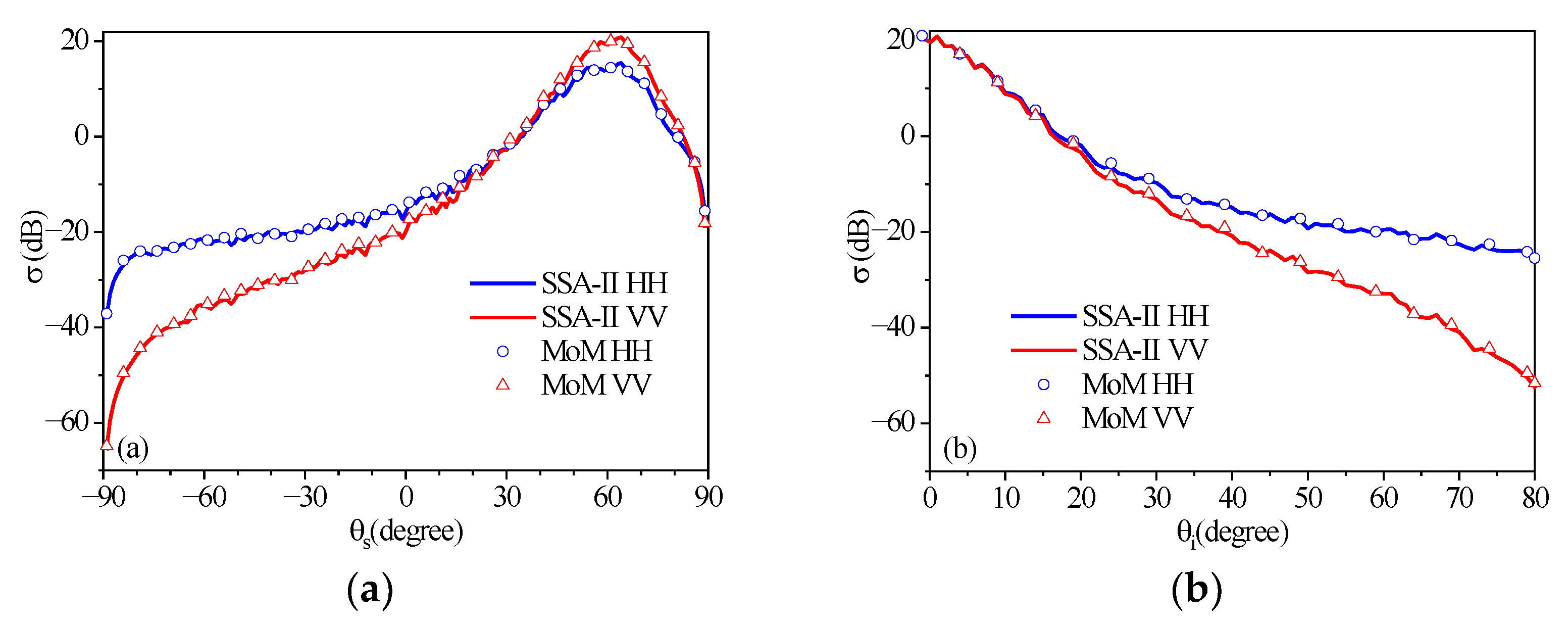
Figure 8 is a comparison of the bistatic and monostatic scattering coefficients of the land–sea junction composite rough surface derived by SSA-II and MoM. In the simulation, the wind speed is $u_{10}=5 \mathrm{m}/\mathrm{s}$ in an upwind direction. The incident angle is ${\theta }_i={30}^{\circ }$, and the incident azimuth angle and scattering azimuth angle are both set to $0^{\circ }$. It can be seen from Figure 8 that the scattering coefficient lines evaluated by SSA-II and MoM show a rather good agreement in both bistatic and monostatic scattering problems.

Figure 9 shows the comparison of the bistatic scattering coefficients of the finite-depth sea surface, the ground surface, and the land–sea junction composite rough surface. The wind speed, incident angle, and incident (scattering) azimuth angle are the same as those in Figure 8. Figure 9 shows that under HH and VV polarizations, the bistatic scattering coefficients of three different types of rough surfaces exhibit spikes in the mirror direction of the incident wave. Regardless of polarization, the bistatic scattering coefficient of a land–sea junction composite rough surface is similar to but smaller than that of a finite-depth sea surface. The bistatic scattering coefficient of the ground surface is much smaller than that of the sea surface and that of the land–sea junction composite rough surface’s overall scattering angles. This is because the ground surface is much flatter than the sea surface in this simulation.

Figure 10 depicts a comparison of the monostatic scattering coefficients of the finite-depth sea surface, the ground surface, and the land–sea junction composite rough surface. The parameters used in the simulation are the same as those in Figure 9. A similar conclusion can be derived from Figure 9 and Figure 10.

The comparison of the bistatic scattering coefficients of a land–sea junction composite rough surface with different root mean square heights is shown in Figure 11. The simulating parameters are the same as those in Figure 9, except that the root mean square of the ground region is set at 0.1 m, 0.3 m, and 0.5 m. From Figure 11, it can be seen that the peak value of the bistatic scattering coefficient decreases with the increase of the root mean square of ground for HH and VV polarizations. However, for HH and VV polarizations, the bistatic scattering coefficient increases with the increase of the root mean square of the ground at the moderate and large scattering angles ($-{40}^{\circ }\le {\theta }_s\le {15}^{\circ }$ and ${40}^{\circ }\le {\theta }_s\le {90}^{\circ }$). This is because as the root mean square increases, so does the degree of ground fluctuation, and more energy is scattered rather than reflected. It can also be found that the scattering coefficient increases with the increase of the root mean square of the ground when the scattering angle ${\theta }_s\ge -{60}^{\circ }$ for cross-polarization.

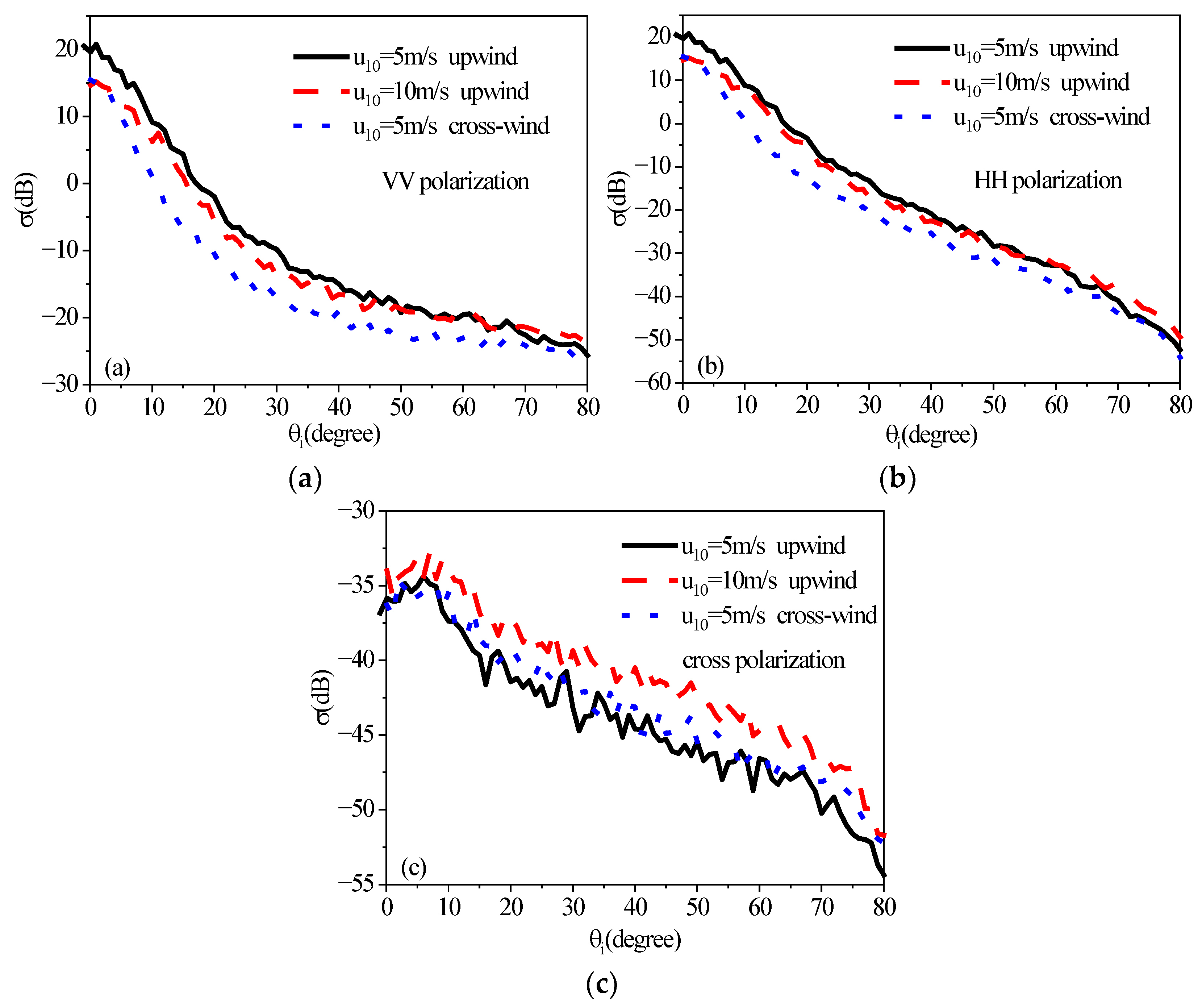
The monostatic scattering coefficients of the land–sea junction composite rough surface versus different wind speeds and wind directions are illustrated in Figure 12. The simulating parameters are the same as in Figure 9, except that the wind speed is set at 5m/s and 10 m/s in upwind and crosswind directions, respectively. As shown in Figure 12, the monostatic scattering coefficient of the land–sea junction composite rough surface decreases with the increase of the wind speed at moderate and small incident angles (${\theta }_i\le {60}^{\circ }$) and increases with the increase of the wind speed at large incident angles (${\theta }_i>{60}^{\circ }$) under HH and VV polarizations. However, for cross-polarization, the monostatic scattering coefficient increases with the increase in wind speed over all incident angles. It can also be found that the monostatic scattering coefficient under cross wind is smaller than that under upwind for co-polarization and is greater than that under upwind for cross-polarization.

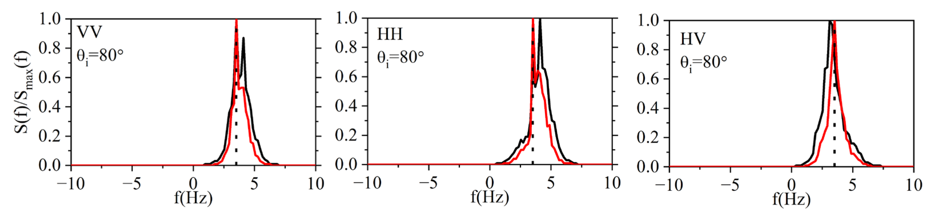
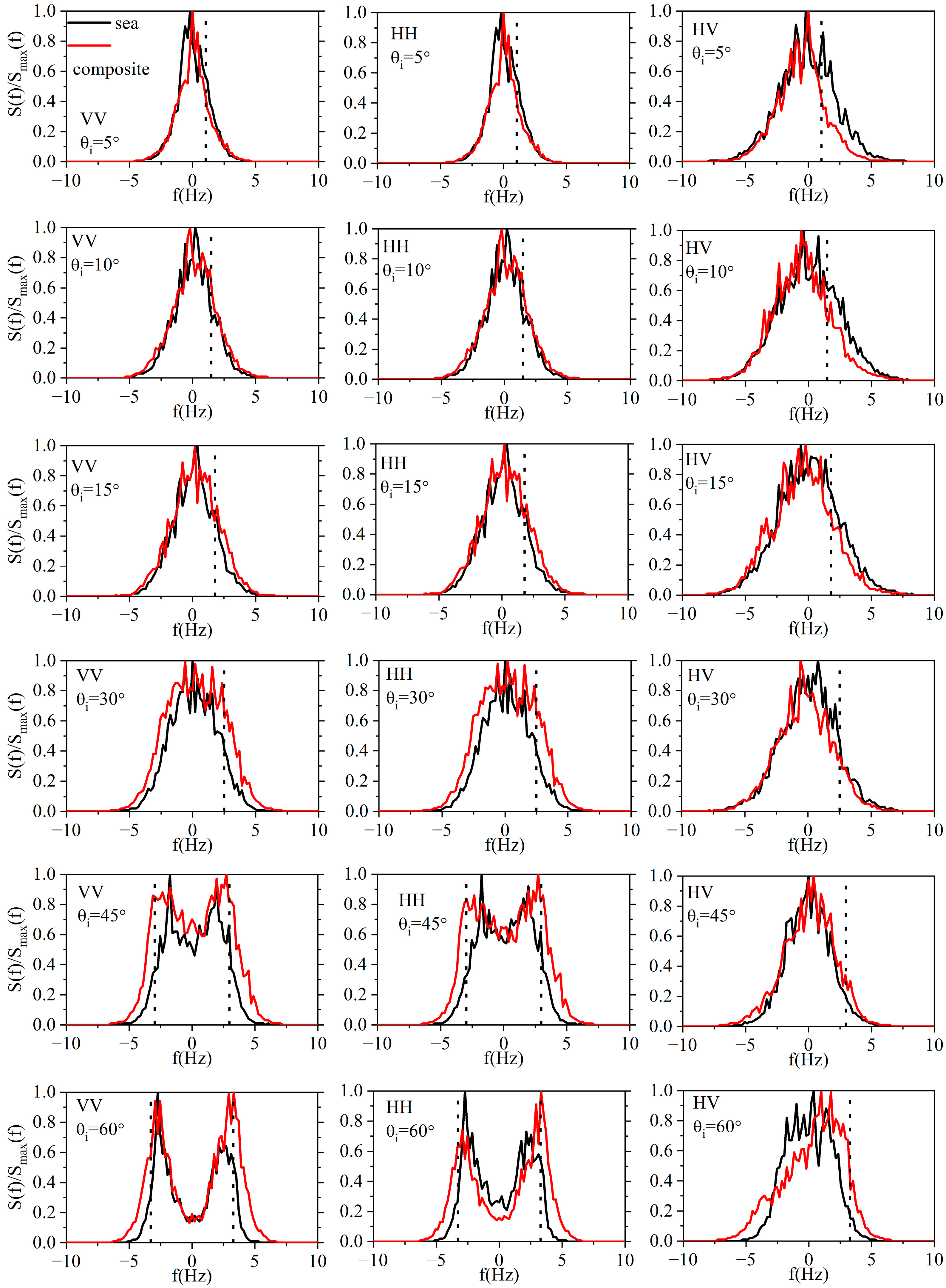
Figure 13 and Figure 14 show the average Doppler spectra of backscattered echoes from the finite-depth sea surface and the land–sea junction composite rough surface. The surface area, the corresponding sample interval, and the incident wave frequency are the same as those in the aforementioned scattering coefficient simulation. The wind speeds are $u_{10}=5 \mathrm{m}/\mathrm{s}$ and $u_{10}=10 \mathrm{m}/\mathrm{s}$ in Figure 13 and Figure 14, respectively. The radar is looking upwind, with the incident angle changing from $5^{\circ }$ to ${80}^{\circ }$. All of the results were averaged over 50 realizations of rough surfaces. Both co-polarization and cross-polarization results are presented. Due to the reciprocity of HV polarization and VH polarization in backscattering, only HV polarized Doppler spectra are presented. The corresponding Bragg frequencies $f_B=\sqrt{g\sin {\theta }_i/(\pi \lambda )}$ are also plotted in Figure 13 and Figure 14 with vertical short-dotted lines.

Figure 13 and Figure 14 show that as the incident angle increases, the bandwidth of the Doppler spectrum widens first and then narrows, and the spectral peak moves closer to the corresponding Bragg frequency for both the finite-depth sea surface and the land–sea junction composite rough surface. Compared with co-polarization, the cross-polarized Doppler spectra are much closer to the corresponding Bragg frequency. This attributes to the fact that the specular reflection plays a leading role in small and moderate incident angles, whereas the Bragg scattering is the primary scattering mechanism in large incident angles. It can also be observed that the Doppler spectra of the land–sea junction composite rough surface are narrower than those of the finite-depth sea surface for both co-polarization and cross-polarization. In addition, it is readily observed that the movement tendency of the Doppler spectral peak is different between co-polarization and cross-polarization. For the co-polarization case, the corresponding frequency of the Doppler spectral peak of the land–sea junction composite rough surface is smaller than that of the finite-depth sea surface, while for the cross-polarization case, the corresponding frequency of the Doppler spectral peak of the land–sea junction composite rough surface is greater than that of the finite-depth sea surface.

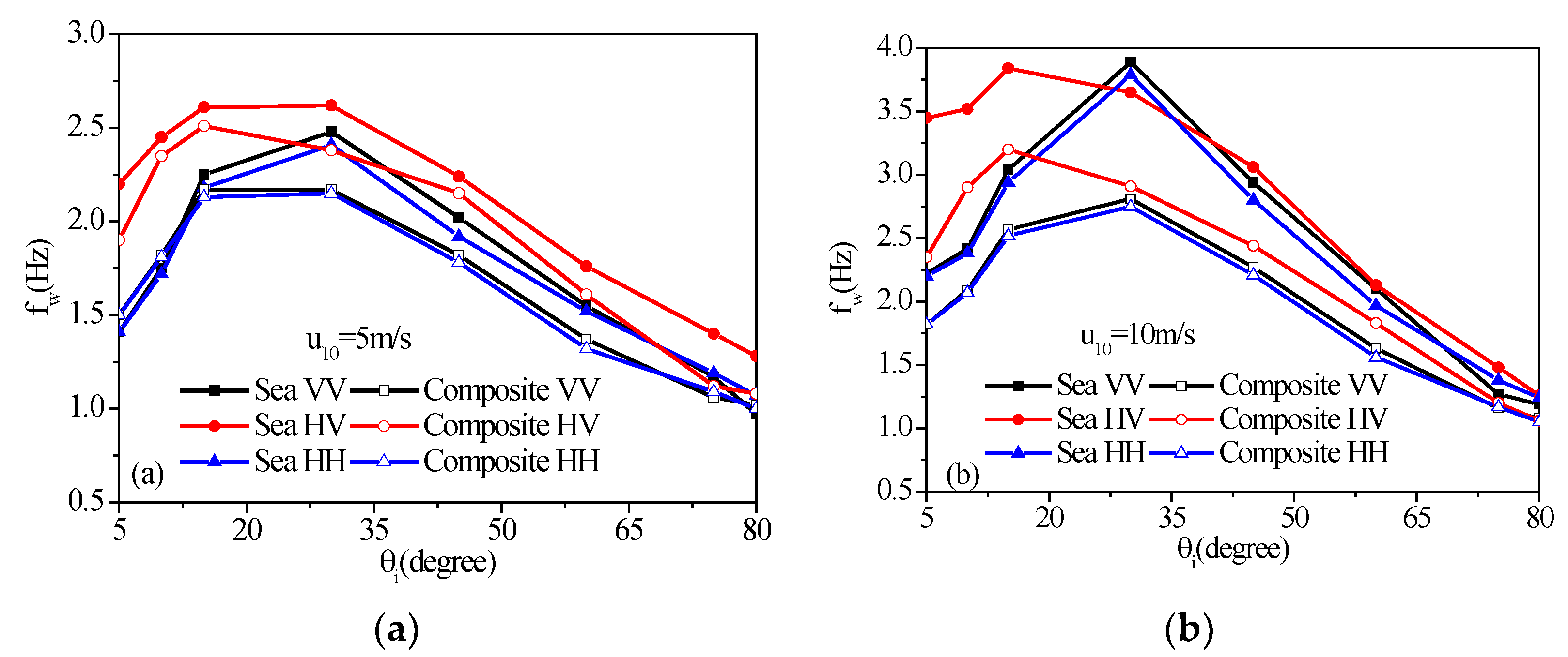
A quantitative comparison of the Doppler shifts (calculated by Equation (16)) and Doppler spectral bandwidths (calculated by Equation (16)) between the finite-depth sea surface and the land–sea junction composite rough surface is shown in Figure 15 and Figure 16, respectively. Similar conclusions can be derived from Figure 15 and Figure 16 as those derived from Figure 13 and Figure 14.

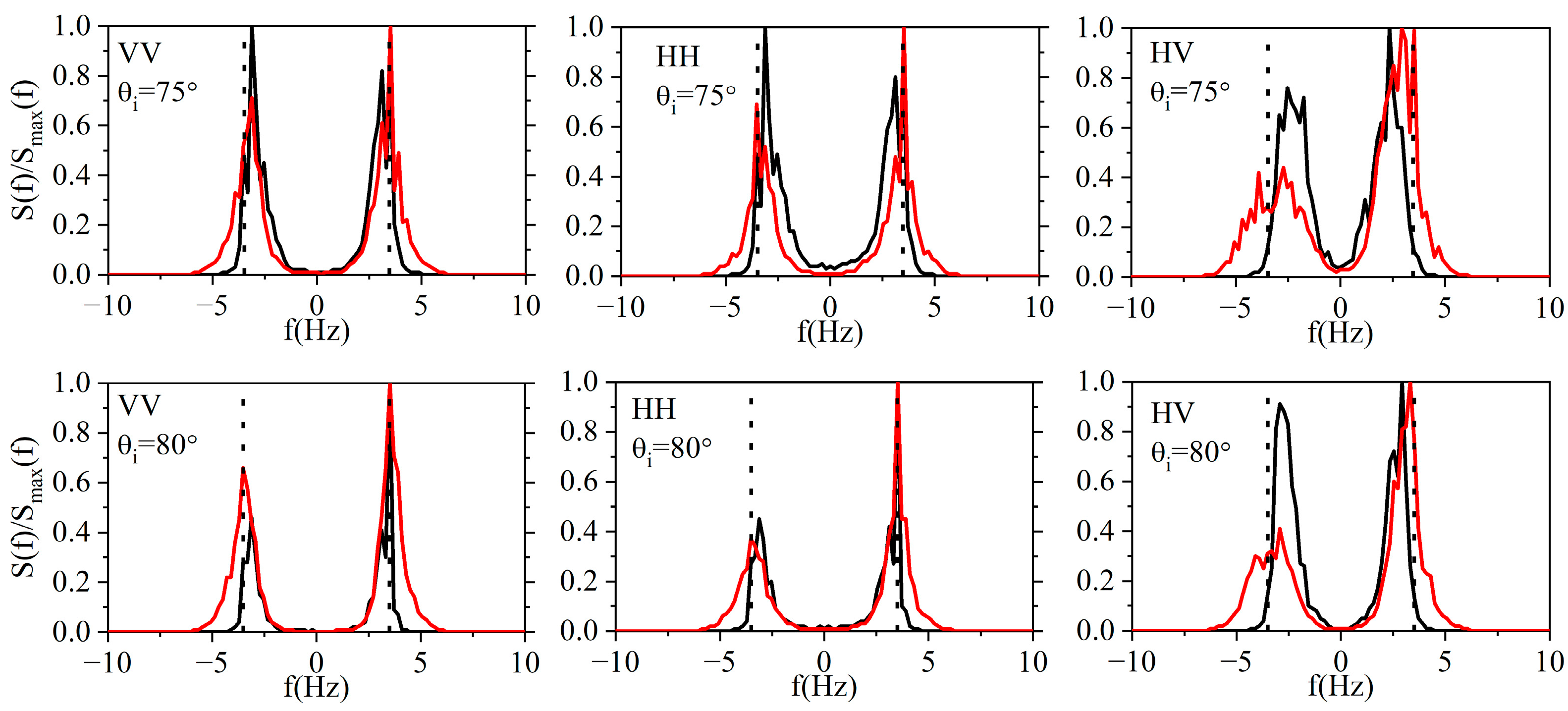
A comparison of average Doppler spectra of backscattered echoes from finite-depth sea surface and land–sea junction composite rough surface under cross wind is shown in Figure 17. The simulating parameters are the same as those in Figure 13, except that the wind direction is set to ${\phi }_w={90}^{\circ }$, which indicates that the radar is looking crosswind. It can be readily observed that only one peak appears when the incident angle is smaller than ${30}^{\circ }$ under co-polarization and smaller than ${60}^{\circ }$ under cross-polarization. However, with the increase in incident angle, two distinct peaks appear for both co- and cross-polarization. These two peaks correspond to the fact that the ocean waves are moving toward and away from the radar. Different from Figure 13, Figure 14, Figure 15 and Figure 16, it can be obviously observed from Figure 17 that the Doppler spectra of the land–sea junction composite rough surface is wider than that of the finite-depth sea surface. In addition, the Doppler spectral peak of the land–sea junction composite rough surface shifts to anhigher frequency relative to that of the finite-depth sea surface.

5. Conclusions

In this paper, a land–sea junction composite rough surface is generated by introducing a weighted arctangent function. The SSA-II, together with a tapered plane incident wave, is applied to obtain the scattering efficient and Doppler spectra of the finite sea surface, the ground surface, and the land–sea junction composite rough surface. The simulation results show that both the bis- and mono-static scattering coefficients of the land–sea junction composite rough surface are smaller than those of the finite sea surface and greater than those of the ground surface for co- and cross-polarizations. By comparing the Doppler spectra of the land–sea junction composite rough surface with that of the finite-depth sea surface, it can be found that a narrowing of the Doppler spectra is observed under upwind direction and a widening of the Doppler spectra is observed under crosswind direction in the presence of the ground surface for both co- and cross-polarizations. Finally, it should be pointed out that only straight shorelines can be modeled with the approach proposed in this paper.

References

1. Tsang, L.; Liao, T.-H.; Tan, S.; Huang, H.; Qiao, T.; Ding, K.-H. Rough surface and volume scattering of soil surfaces, ocean surfaces, snow, and vegetation based on numerical maxwell model of 3-D simulations. IEEE J. Sel. Top. Appl. Earth Obs. Remote Sens. 2017, 10, 4703–4720. [Google Scholar] [CrossRef]
2. Hao, J.W.; Song, W.; Sheng, X.Q. Efficient algorithm for calculating backscattering from two-dimensional rough sea surface under low grazing angle. In Proceedings of the IGARSS 2016 IEEE International Geoscience and Remote Sensing Symposium, Beijing, China, 10–15 July 2016. [Google Scholar]
3. Khankhoje, U.K.; Padhy, S. Stochastic Solutions to Rough Surface Scattering Using the Finite Element Method. IEEE Trans. Antennas Propag. 2017, 65, 4170–4180. [Google Scholar] [CrossRef]
4. Li, J.; Guo, L.X.; Zeng, H.; Han, X.B. Message-passing-interface-based parallel FDTD investigation on the EM scattering from a 1-D rough sea surface using uniaxial perfectly matched layer absorbing boundary. J. Opt. Soc. Am. A Opt. Image Sci. Vis. 2009, 26, 1494–1502. [Google Scholar] [CrossRef] [PubMed]
5. Li, J.; Guo, L.X.; Zeng, H. FDTD investigation on bistatic scattering from two-dimensional rough surface with UPML absorbing condition. Waves Random Complex Media 2009, 19, 418–429. [Google Scholar] [CrossRef]
6. Li, J.; Guo, L.X.; Zeng, H. FDTD investigation on electromagnetic scattering from two-layered rough surfaces under UPML absorbing condition. Chin. Phys. Lett. 2009, 26, 034101. [Google Scholar] [CrossRef]
7. Guo, X.Y.; Liu, Y.; Zhou, H.J.; Xia, M.Y. Simulation of transient scattering from ocean surface with ship wake. In Proceedings of the 2017 IEEE International Conference on Computational Electromagnetics, ICCEM 2017, Kumamoto, Japan, 8–10 March 2017; pp. 78–80. [Google Scholar]
8. Yang, J.S.; Du, Y.; Shi, J.C. Polarimetric Simulations of Bistatic Scattering from Perfectly Conducting Ocean Surfaces with 3 m/s Wind Speed at L-Band. IEEE J. Sel. Top. Appl. Earth Obs. Remote Sens. 2016, 9, 1176–1186. [Google Scholar] [CrossRef]
9. Afifi, S.; Dusseaux, R. Scattering from 2-D Perfect Electromagnetic Conductor Rough Surface: Analysis with the Small Perturbation Method and the Small-Slope Approximation. IEEE Trans. Antennas Propag. 2018, 66, 340–346. [Google Scholar] [CrossRef]
10. Li, H.; Johnson, J.T. On the Amplitude Distributions of Bistatic Scattered Fields from Rough Surfaces. IEEE Trans. Geosci. Remote Sens. 2017, 55, 6883–6892. [Google Scholar] [CrossRef]
11. Voronovich, A.G.; Zavorotny, V.U. The transition from weak to strong diffuse radar bistatic scattering from rough ocean surface. IEEE Trans. Antennas Propag. 2017, 65, 6029–6034. [Google Scholar] [CrossRef]
12. Wang, J.N.; Xu, X.J. Doppler Simulation and Analysis for 2-D Sea Surfaces Up to Ku-Band. IEEE Trans. Geosci. Remote Sens. 2016, 54, 466–478. [Google Scholar] [CrossRef]
13. Zamani, H.; Tavakoli, A.; Dehmollaian, M. Second-Order Perturbative Solution of Cross-Polarized Scattering from Multilayered Rough Surfaces. IEEE Trans. Antennas Propag. 2016, 64, 1877–1890. [Google Scholar] [CrossRef]
14. Zamani, H.; Tavakoli, A.; Dehmollaian, M. Scattering from Layered Rough Surfaces: Analytical and Numerical Investigations. IEEE Trans. Geosci. Remote Sens. 2016, 54, 3685–3692. [Google Scholar] [CrossRef]
15. Burkholder, R.J.; Johnson, J.T.; Sanamzadeh, M.; Tsang, L.; Tan, S. Microwave Thermal Emission Characteristics of a Two-Layer Medium with Rough Interfaces Using the Second-Order Small Perturbation Method. IEEE Geosci. Remote Sens. Lett. 2017, 14, 1780–1784. [Google Scholar] [CrossRef]
16. Wei, Y.W.; Guo, L.X.; Chai, S.R.; Wang, A.Q. A new semi-deterministic facet model for electromagnetic scattering from ocean-like surface. In Proceedings of the 2013 33rd IEEE International Geoscience and Remote Sensing Symposium, IGARSS 2013, Melbourne, VIC, Australia, 21–26 July 2013; pp. 1372–1375. [Google Scholar]
17. Zeng, J.Y.; Chen, K.S.; Bi, H.Y.; Zhao, T.J.; Yang, X.F. A Comprehensive Analysis of Rough Soil Surface Scattering and Emission Predicted by AIEM with Comparison to Numerical Simulations and Experimental Measurements. IEEE Trans. Geosci. Remote Sens. 2017, 55, 1696–1708. [Google Scholar] [CrossRef]
18. Wang, T.; Tong, C.M. An Improved Facet-Based TSM for Electromagnetic Scattering from Ocean Surface. IEEE Geosci. Remote Sens. Lett. 2018, 15, 644–648. [Google Scholar] [CrossRef]
19. Awada, A.; Ayari, M.Y.; Khenchaf, A.; Coatanhay, A. Bistatic scattering from an anisotropic sea surface: Numerical comparison between the first-order SSA and the TSM models. Waves Random Complex Media 2006, 16, 383–394. [Google Scholar] [CrossRef]
20. Khenchaf, A. Bistatic scattering and depolarization by randomly rough surfaces: Application to the natural rough surfaces in X-band. Waves Random Media 2001, 11, 61–89. [Google Scholar] [CrossRef]
21. Vaitilingom, L.; Khenchaf, A. Radar cross sections of sea and ground clutter estimated by two scale model and small slope approximation in HF-VHF bands. Prog. Electromagn. Res. B 2011, 29, 311–338. [Google Scholar] [CrossRef]
22. Zheng, H.; Zhang, J.; Zhang, Y.; Khenchaf, A.; Wang, Y. Theoretical Study on Microwave Scattering Mechanisms of Sea Surfaces Covered with and without Oil Film for Incidence Angle Smaller Than 30. IEEE Trans. Geosci. Remote Sens. 2021, 59, 37–46. [Google Scholar] [CrossRef]
23. Sajjad, N.; Khenchaf, A.; Coatanhay, A. Depolarization of electromagnetic waves from bare soil surfaces. Sci. Comput. Elect. Eng. Springer Math. Ind. 2012, 16, 107–115. [Google Scholar]
24. Zou, G.X.; Tong, C.M.; Sun, H.L.; Peng, P. Research on electromagnetic scattering characteristics of combined conducting and dielectric target above coastal environment. IEEE Access 2020, 8, 169286–169303. [Google Scholar] [CrossRef]
25. Sun, H.L.; Tong, C.M.; Zou, G.X. High Efficiency Iterative Solver for Modeling Composite Rough Surface Electromagnetic Scattering. Electromagnetics 2017, 37, 113–126. [Google Scholar] [CrossRef]
26. Zou, G.X.; Tong, C.M.; Sun, H.L.; Wang, T.; Peng, P. A hybrid method for electromagnetic scattering from target above composite rough surface of ground and near sea in adjacent region. Electromagnetics 2018, 38, 415–437. [Google Scholar] [CrossRef]
27. Zou, G.X.; Tong, C.M.; Sun, H.L.; Wang, T.; Tian, G.L. Modeling and electromagnetic scattering of composite rough surface of island in deep sea. In Proceedings of the 2017 International Applied Computational Electromagnetics Society Symposium in China, ACES-China 2017, Suzhou, China, 1–4 August 2017. [Google Scholar]
28. Zou, G.X.; Tong, C.M.; Huang, Y.L.; Sun, H.L.; Wang, T. Modeling and electromagnetic scattering of ground and near sea in adjacent region with fractal borderline. In Proceedings of the 2017 7th International Workshop on Computer Science and Engineering, WCSE 2017, Beijing, China, 25–27 June 2017; pp. 1055–1060. [Google Scholar]
29. Chai, S.R.; Li, H.; Li, J. Simulation of Radar Scattering Characteristics of a Target Located in Ground-Sea Junction Area Based on Improved SBR Algorithm. In Proceedings of the 2020 Cross Strait Radio Science and Wireless Technology Conference, CSRSWTC 2020, Fuzhou, China, 13–16 December 2020. [Google Scholar]
30. McCormick, M.E. Ocean Engineering Wave Mechanics; John Wiley & Sons: Hoboken, NJ, USA, 1973. [Google Scholar]
31. Voronovich, A.G.; Zavorotny, V.U. Theoretical model for scattering of radar signals in Ku- and C-bands from a rough sea surface with breaking waves. Waves Random Media 2001, 11, 247–269. [Google Scholar] [CrossRef]
32. Wentz, F.J.; Peteherych, S.; Thomas, L.A. A model function for ocean radar cross sections at 14.6 GHz. J. Geophys. Res. Ocean. 1984, 89, 3689–3704. [Google Scholar] [CrossRef]
33. Apel, J.R. Principles of Ocean Physics; Academic Press: Cambridge, MA, USA, 1987. [Google Scholar]
Figure 1. Finite-depth sea spectra for different water depths: (a) S finite ( ω ) ; (b) S finite ( k ) .
Remotesensing 15 00836 g001
Figure 2. Simulated finite-depth sea surface under wind speed u 10 = 10   m / s .
Remotesensing 15 00836 g002
Figure 3. Composite plate derived by introducing the weighted arctangent function.
Remotesensing 15 00836 g003
Figure 4. Simulated land–sea junction composite rough surface l x = l y = 3.0   m δ = 0.1   m .
Remotesensing 15 00836 g004
Figure 5. Simulated land–sea junction composite rough surface l x = l y = 10.0   m δ = 1.0   m .
Remotesensing 15 00836 g005
Figure 6. Geometry of the land–sea junction composite rough surface scattering problem and notation.
Remotesensing 15 00836 g006
Figure 7. Validation of SSA-II by comparing with experimental data: (a) u 10 = 5   m / s , X = 100   km ; (b) u 10 = 10   m / s , X = 300   km .
Remotesensing 15 00836 g007
Figure 8. Validation of SSA-II by comparing with MoM results: (a) bistatic and (b) monostatic.
Remotesensing 15 00836 g008
Figure 9. Comparison of the bistatic scattering coefficients of the finite-depth sea surface, the ground surface, and the land–sea junction composite rough surface at different polarizations. (a) VV, (b) HH, (c) HV, and (d) VH.
Remotesensing 15 00836 g009
Figure 10. Comparison of the monostatic scattering coefficients of the finite-depth sea surface, the ground surface, and the land–sea junction composite rough surface at different polarizations. (a) VV, (b) HH, and (c) cross-polarization.
Remotesensing 15 00836 g010
Figure 11. Comparison of the bistatic scattering coefficients of a land–sea junction composite rough surface with different root mean square heights at different polarizations. (a) VV, (b) HH, (c) HV, and (d) VH.
Remotesensing 15 00836 g011aRemotesensing 15 00836 g011b
Figure 12. Comparison of the monostatic scattering coefficients of the land–sea junction composite rough surface with different wind speeds and wind directions at different polarizations. (a) VV, (b) HH, and (c) cross-polarization.
Remotesensing 15 00836 g012
Figure 13. Average Doppler spectra of backscattered echoes from the finite-depth sea surface and the land–sea junction composite rough surface at various incident angles with a wind speed of u 10 = 5   m / s . The left column, the middle column, and the right column is for VV, HH, and HV polarizations, respectively. The vertical short-dotted lines represent Bragg frequencies. The radar is looking upwind.
Remotesensing 15 00836 g013
Figure 14. Similar to Figure 13, but with wind speed u 10 = 10   m / s .
Remotesensing 15 00836 g014aRemotesensing 15 00836 g014b
Figure 15. Comparison of the Doppler shifts between the finite-depth sea surface and the land–sea junction composite rough surface. (a) u 10 = 5   m / s and (b) u 10 = 10   m / s .
Remotesensing 15 00836 g015
Figure 16. Comparison of the Doppler spectral bandwidths between the finite-depth sea surface and the land–sea junction composite rough surface. (a) u 10 = 5   m / s and (b) u 10 = 10   m / s .
Remotesensing 15 00836 g016
Figure 17. Similar to Figure 13, except that the wind direction is φ w = 90 .
Remotesensing 15 00836 g017aRemotesensing 15 00836 g017b
Disclaimer/Publisher’s Note: The statements, opinions and data contained in all publications are solely those of the individual author(s) and contributor(s) and not of MDPI and/or the editor(s). MDPI and/or the editor(s) disclaim responsibility for any injury to people or property resulting from any ideas, methods, instructions or products referred to in the content.