

A Review of Data Augmentation Methods of Remote Sensing Image Target Recognition


Abstract
:
1. Introduction
2. Data-Based Data Augmentation Methods
2.1. One-Sample Transform
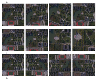
2.1.1. Geometric Transformations
2.1.2. Sharpness Transformation
2.1.3. Noise Disturbance
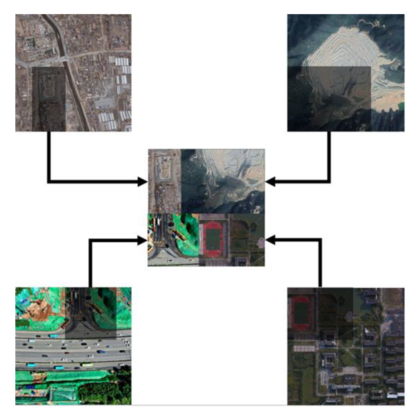
2.1.4. Random Erase
2.2. Multi-Sample Synthesis
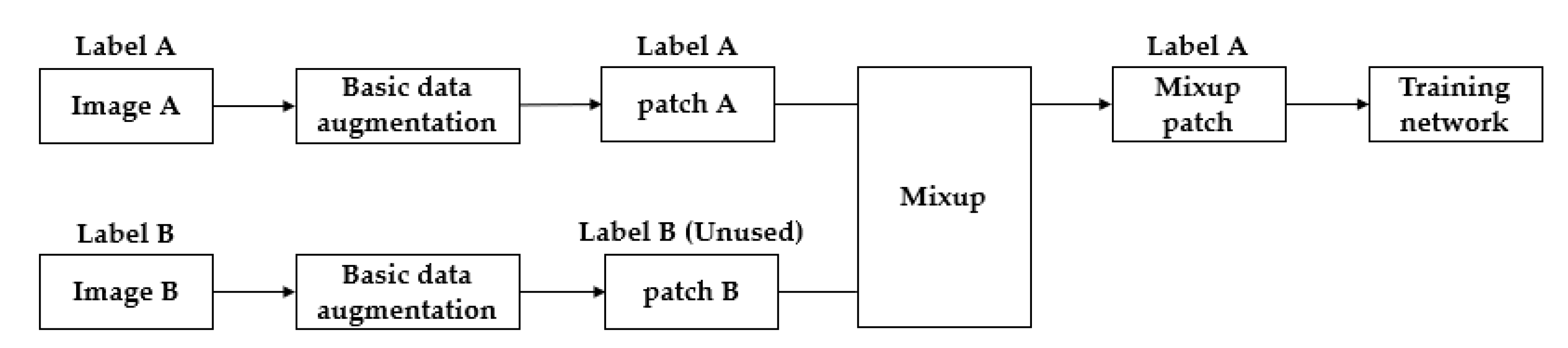
2.2.1. Spatial Information Synthesis
- (1)
- Linear stacking method of multiple images
- ➀
- Mixup
- ➁
- Between-Class (BC)
- ➂
- Sample Pairing
- ➃
- CutMix
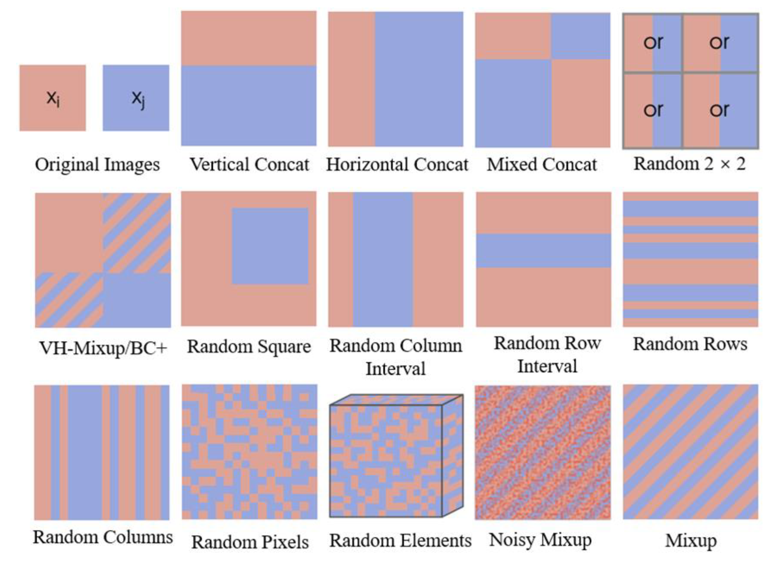
- (2)
- Nonlinear blending method of multiple images
2.2.2. Feature Space Information Synthesis
- (1)
- CNN
- (2)
- SMOTE
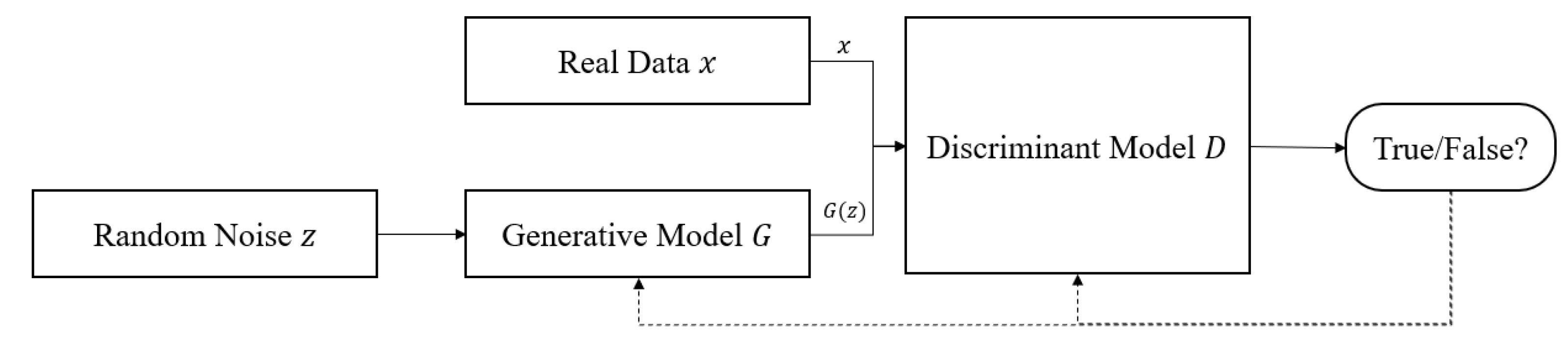
2.3. Deep Generative Models
2.3.1. Approximation Method
- (1)
- RBM
- ➀
- DBN
- ➁
- HM
- ➂
- DBM
- (2)
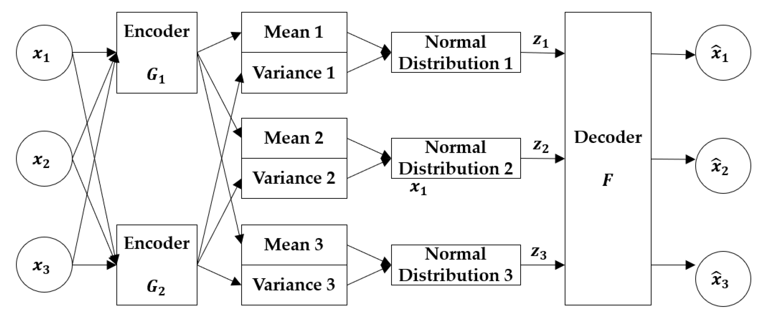
- VAE
- ➀
- IWAE
- ➁
- ADGM
- ➂
- AAE
- ➃
- MAE
2.3.2. Implicit Method
2.3.3. Deformation Method
- (1)
- Flow Model
- ➀
- Normalizing Flow Model
- ➁
- i-ResNet
- ➂
- Variational Inference with the Flow
- (2)
- Autoregressive Model
- ➀
- NADE
- ➁
- PixelRNN
- ➂
- MADE
2.4. Virtual Sample Generation
3. Network-Based Data Augmentation Methods
3.1. Network Strategy
3.1.1. Transfer Learning
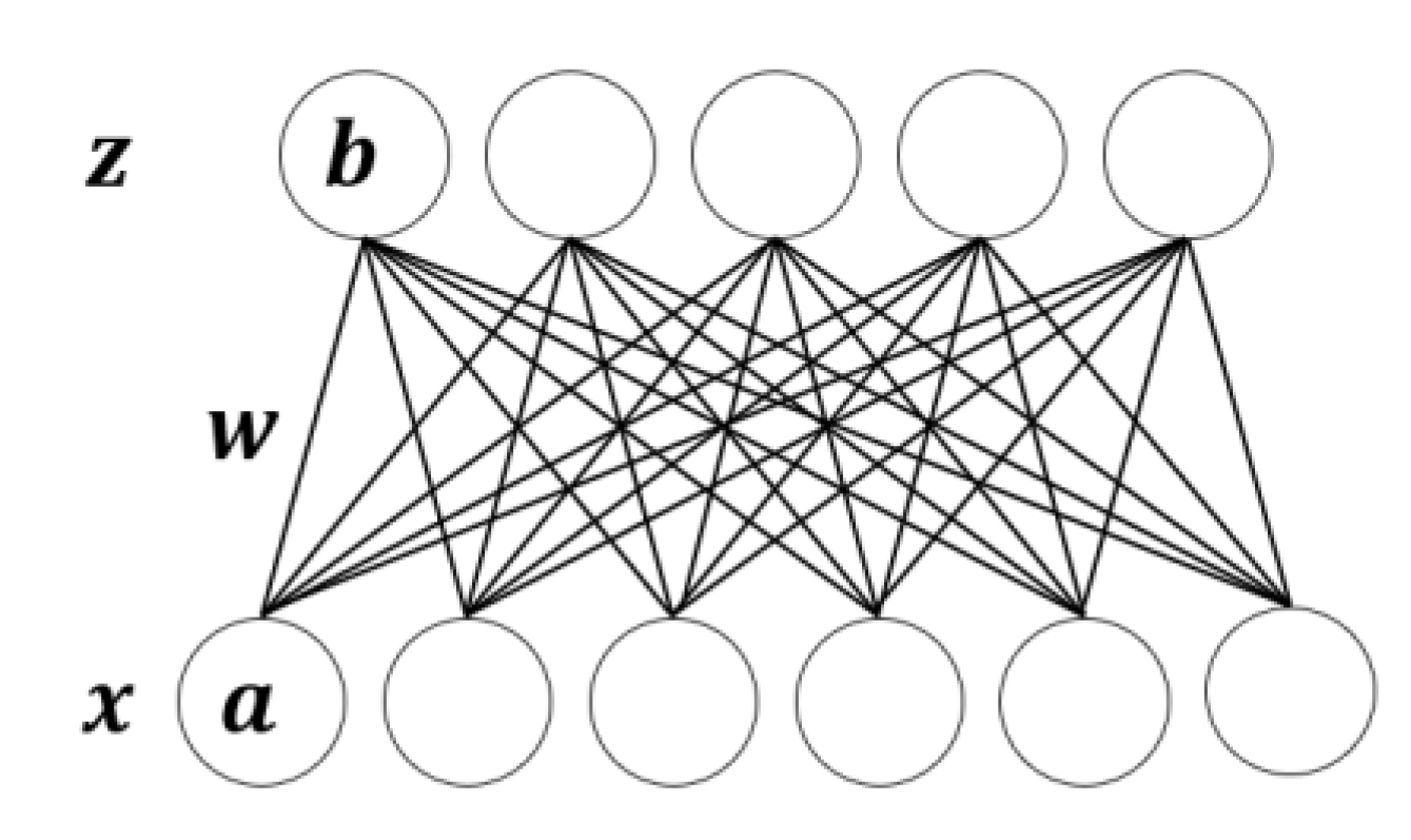
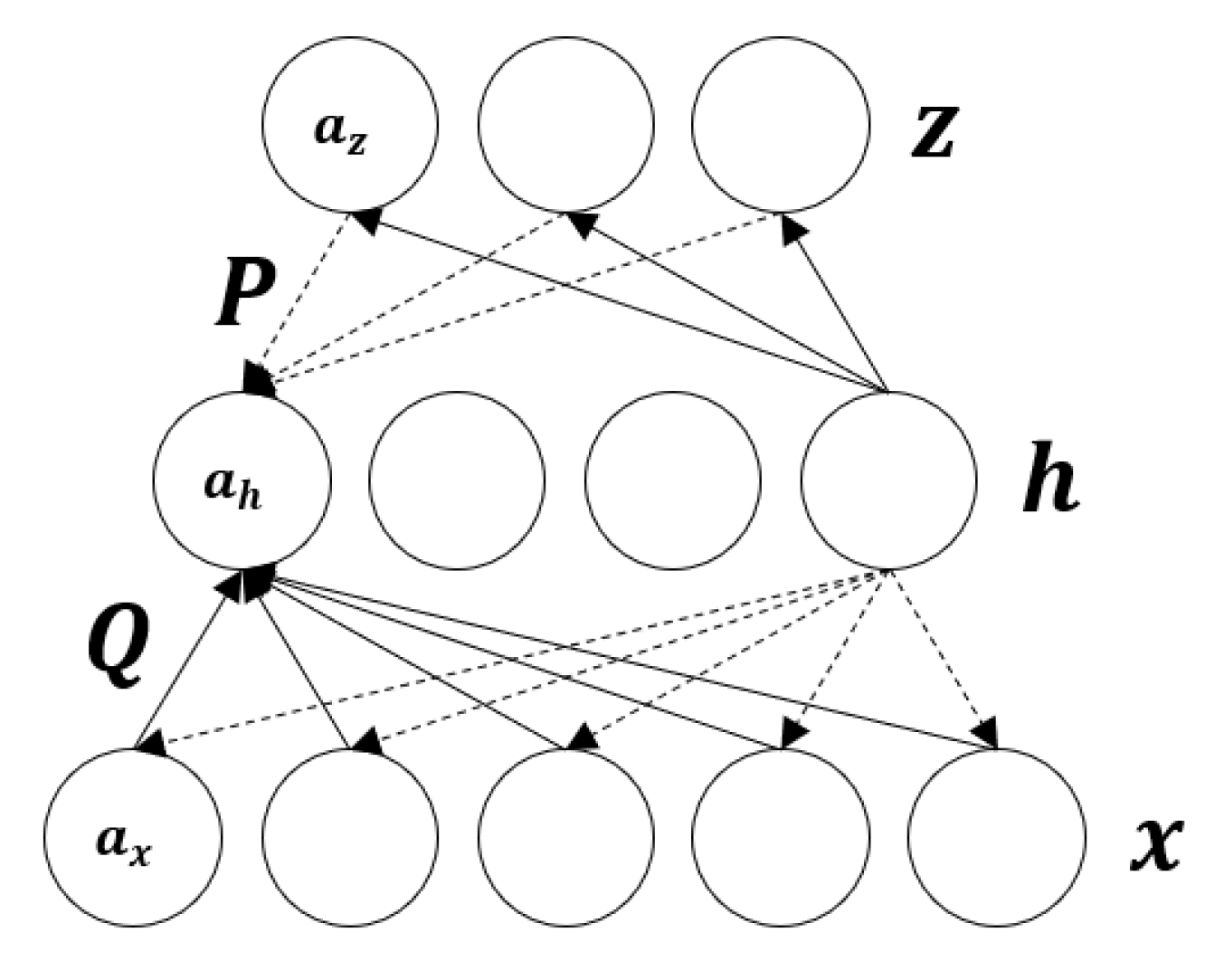
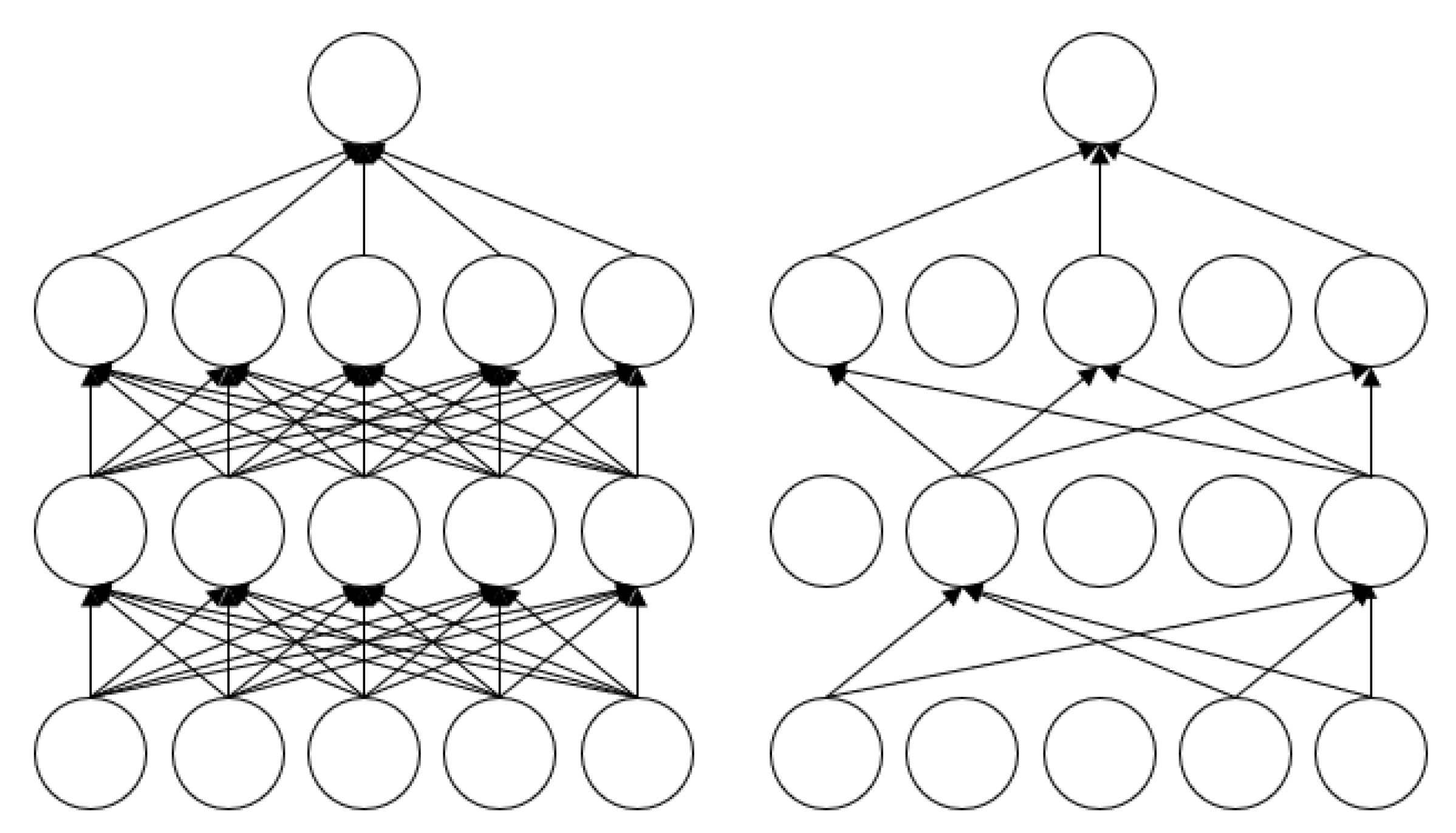
3.1.2. Regularization
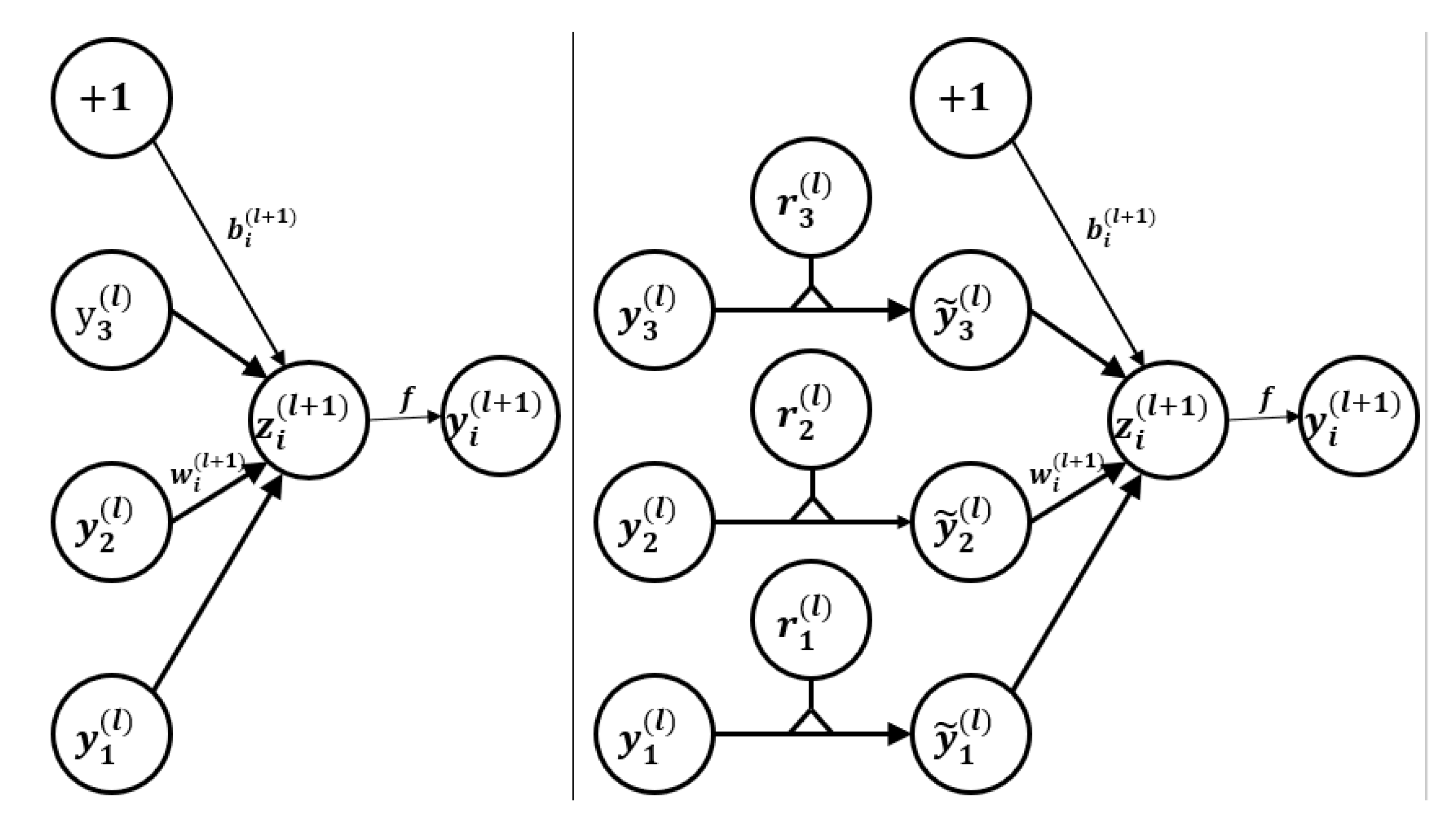
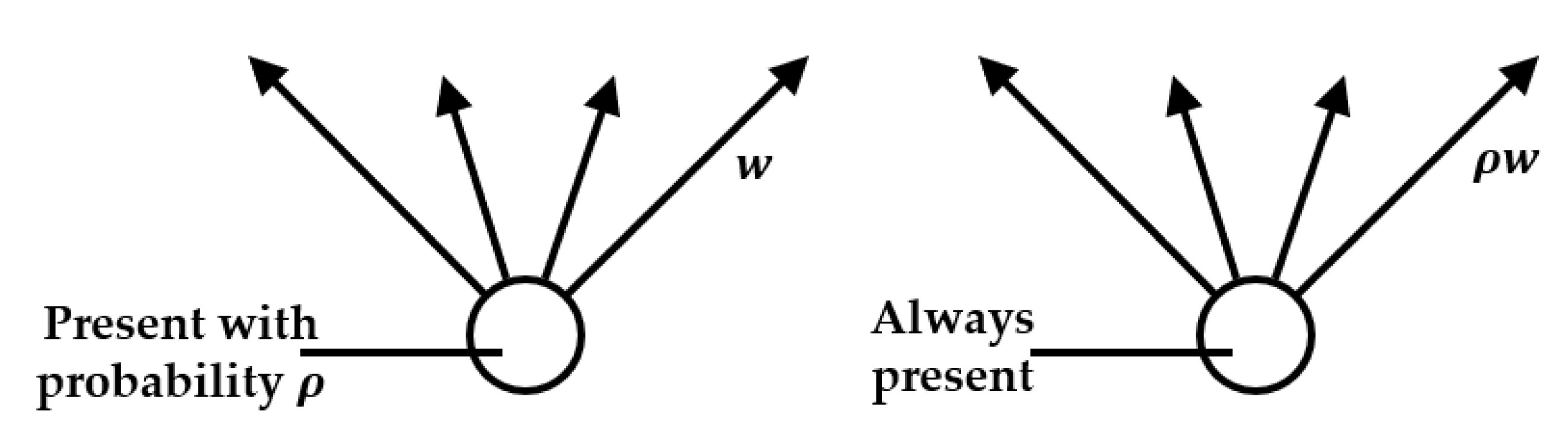
- (1)
- Dropout workflow
- (2)
- Use of Dropout in Neural Networks
- ➀
- During the training model phase
- ➁
- During the testing phase
3.2. Learning Strategy
3.2.1. Meta-Learning
3.2.2. Reinforcement Learning
4. Challenges and Future Directions
5. Conclusions
Author Contributions
Funding
Data Availability Statement
Conflicts of Interest
References
- Zhang, S.; Cheng, Q.; Chen, D.; Zhang, H. Image Target Recognition Model of Multichannel Structure Convolutional Neural Network Training Automatic Encoder. IEEE Access 2020, 8, 113090–113103. [Google Scholar] [CrossRef]
- Zhou, Y.; Zhu, Z.; Ding, Q. Port Target Recognition of Remote Sensing Image. J. Nanjing Univ. Aeronaut. Astronaut. 2008, 40, 350–353. [Google Scholar]
- He, J.; Guo, Y.; Yuan, H. Ship Target Automatic Detection Based on Hypercomplex Flourier Transform Saliency Model in High Spatial Resolution Remote-Sensing Images. Sensors 2020, 20, 2536. [Google Scholar] [CrossRef] [PubMed]
- Huang, X.; Zhang, L.; Zhu, T. Building Change Detection from Multitemporal High-Resolution Remotely Sensed Images Based on a Morphological Building Index. IEEE J. Sel. Top. Appl. Earth Obs. Remote Sens. 2013, 7, 105–115. [Google Scholar] [CrossRef]
- Shu, C.; Sun, L. Automatic target recognition method for multitemporal remote sensing image. Open Phys. 2020, 18, 170–181. [Google Scholar] [CrossRef]
- Jin, L.; Kuang, X.; Huang, H.; Qin, Z.; Wang, Y. Over-fitting Study of Artificial Neural Network Prediction Model. J. Meteorol. 2004, 62, 62–70. [Google Scholar]
- Lee, J.-G.; Jun, S.; Cho, Y.-W.; Lee, H.; Kim, G.B.; Seo, J.B.; Kim, N. Deep Learning in Medical Imaging: General Overview. Korean J. Radiol. 2017, 18, 570–584. [Google Scholar] [CrossRef]
- Zhai, J. Why Not Recommend a Small Sample for Further Study? 2018. Available online: https://www.zhihu.com/question/29633459/answer/45049798 (accessed on 20 November 2022).
- Vogel-Walcutt, J.; Gebrim, J.; Bowers, C.; Carper, T.; Nicholson, D. Cognitive load theory vs. constructivist approaches: Which best leads to efficient, deep learning? J. Comput. Assist. Learn. 2010, 27, 133–145. [Google Scholar] [CrossRef]
- Simard, P.Y.; LeCun, Y.A.; Denker, J.S.; Victorri, B. Transformation Invariance in Pattern Recognition—Tangent Distance and Tangent Propagation. In Neural Networks: Tricks of the Trade; Springer: Berlin/Heidelberg, Germany, 2012; pp. 235–269. [Google Scholar]
- Abu Alhaija, H.; Mustikovela, S.K.; Mescheder, L.; Geiger, A.; Rother, C. Augmented Reality Meets Computer Vision: Efficient Data Generation for Urban Driving Scenes. Int. J. Comput. Vis. 2018, 126, 961–972. [Google Scholar] [CrossRef]
- Fernández, A.; García, S.; Galar, M.; Prati, R.C.; Krawczyk, B.; Herrera, F. Learning from Imbalanced Data Sets; Springer International Publishing: Cham, Switzerland, 2018. [Google Scholar] [CrossRef]
- Mikolajczyk, A.; Grochowski, M. Data augmentation for improving deep learning in image classification problem. In Proceedings of the International Interdisciplinary PhD Workshop (IIPhDW), Swinoujscie, Poland, 9–12 May 2018; pp. 117–122. [Google Scholar]
- Nalepa, J.; Marcinkiewicz, M.; Kawulok, M. Data Augmentation for Brain-Tumor Segmentation: A Review. Front. Comput. Neurosci. 2019, 13, 83. [Google Scholar] [CrossRef]
- Shorten, C.; Khoshgoftaar, T.M. A survey on Image Data Augmentation for Deep Learning. J. Big Data 2019, 6, 60. [Google Scholar] [CrossRef]
- Lemley, J.; Corcoran, P. Deep Learning for Consumer Devices and Services 4—A Review of Learnable Data Augmentation Strategies for Improved Training of Deep Neural Networks. IEEE Consum. Electron. Mag. 2020, 9, 55–63. [Google Scholar] [CrossRef]
- Chlap, P.; Min, H.; Vandenberg, N.; Dowling, J.; Holloway, L.; Haworth, A. A review of medical image data augmentation techniques for deep learning applications. J. Med. Imaging Radiat. Oncol. 2021, 65, 545–563. [Google Scholar] [CrossRef]
- Song, Y.; Wang, T.; Mondal, S.K.; Sahoo, J.P. A Comprehensive Survey of Few-shot Learning: Evolution, Applications, Challenges, and Opportunities. arXiv 2022, arXiv:2205.06743. [Google Scholar] [CrossRef]
- Taylor, L.; Nitschke, G. Improving Deep Learning with Generic Data Augmentation. In Proceedings of the 2018 IEEE Symposium Series on Computational Intelligence (SSCI), Bangalore, India, 18–21 November 2018; pp. 1542–1547. [Google Scholar]
- Ma, D.A.; Tang, P.; Zhao, L.J.; Zhang, Z. Review of Data Augmentation for Image in Deep Learning. J. Image Graph. 2021, 26, 0487–0502. [Google Scholar]
- Zhang, W.; Cao, Y. A new data augmentation method of remote sensing dataset based on Class Activation Map. J. Phys. Conf. Ser. 2021, 1961, 012023. [Google Scholar] [CrossRef]
- Ledig, C.; Theis, L.; Huszár, F.; Caballero, J.; Cunningham, A.; Acosta, A.; Shi, W. Photo-Realistic Single Image Super-Resolution Using a Generative Adversarial Network. In Proceedings of the IEEE Conference on Computer Vision and Pattern Recognition, Honolulu, HI, USA, 21–26 July 2017; pp. 4681–4690. [Google Scholar]
- Ding, J.; Chen, B.; Liu, H.; Huang, M. Convolutional Neural Network with Data Augmentation for SAR Target Recognition. IEEE Geosci. Remote Sens. Lett. 2016, 13, 364–368. [Google Scholar] [CrossRef]
- Wang, Y.K.; Zhang, P.Y.; Yan, Y.H. Data Enhancement Technology of Language Model Based on Countermeasure Training Strategy. J. Autom. 2018, 44, 126–135. [Google Scholar]
- Ma, D.; Tang, P.; Zhao, L. SiftingGAN: Generating and Sifting Labeled Samples to Improve the Remote Sensing Image Scene Classification Baseline In Vitro. IEEE Geosci. Remote Sens. Lett. 2019, 16, 1046–1050. [Google Scholar] [CrossRef]
- DeVries, T.; Taylor, G.W. Improved Regularization of Convolutional Neural Networks with Cutout. arXiv 2017, arXiv:1708.04552. [Google Scholar]
- Su, N. A Data Augmentation Strategy Based on Simulated Samples for Ship Detection in RGB Remote Sensing Images. ISPRS Int. J. Geo-Inf. 2019, 8, 276. [Google Scholar]
- Wang, Z.; Du, L.; Mao, J.; Liu, B.; Yang, D. SAR Target Detection Based on SSD with Data Augmentation and Transfer Learning. IEEE Geosci. Remote Sens. Lett. 2019, 16, 150–154. [Google Scholar] [CrossRef]
- Scott, G.J.; England, M.R.; Starms, W.A.; Marcum, R.A.; Davis, C.H. Training Deep Convolutional Neural Networks for Land–Cover Classification of High-Resolution Imagery. IEEE Geosci. Remote Sens. Lett. 2017, 14, 549–553. [Google Scholar] [CrossRef]
- Chapelle, O.; Weston, J.; Bottou, L.; Vapnik, V. Vicinal Risk Minimization. Adv. Neural Inf. Process. Syst. 2000, 13. [Google Scholar]
- Vapnik, V.N. An overview of statistical learning theory. IEEE Trans. Neural Netw. 1999, 10, 988–999. [Google Scholar] [CrossRef]
- Zhang, H.; Cisse, M.; Dauphin, Y.N.; Lopez-Paz, D. Mixup: Beyond Empirical Risk Minimization. arXiv 2017, arXiv:1710.09412. [Google Scholar]
- Yan, P.; He, F.; Yang, Y.; Hu, F. Semi-Supervised Representation Learning for Remote Sensing Image Classification Based on Generative Adversarial Networks. IEEE Access 2020, 8, 54135–54144. [Google Scholar] [CrossRef]
- Tokozume, Y.; Ushiku, Y.; Harada, T. Between-Class Learning for Image Classification. In Proceedings of the 2018 IEEE/CVF Conference on Computer Vision and Pattern Recognition, Salt Lake City, UT, USA, 18–23 June 2018; pp. 5486–5494. [Google Scholar]
- Inoue, H. Data Augmentation by Pairing Samples for Images Classification. arXiv 2018, arXiv:1801.02929. [Google Scholar]
- Yan, Y. Data Augmentation Method in Deep Learning. 2018. Available online: https://www.jianshu.com/p/99450dbdadcf (accessed on 2 November 2022).
- Yun, S.; Han, D.; Oh, S.J.; Chun, S.; Choe, J.; Yoo, Y. CutMix: Regularization Strategy to Train Strong Classifiers with Localizable Features. arXiv 2019, arXiv:1905.04899. [Google Scholar]
- Summers, C.; Dinneen, M.J. Improved Mixed-Example Data Augmentation. In Proceedings of the 2019 IEEE Winter Conference on Applications of Computer Vision (WACV), Waikoloa Village, HI, USA, 7–11 January 2019; pp. 1262–1270. [Google Scholar]
- Takahashi, R.; Matsubara, T.; Uehara, K. Data Augmentation Using Random Image Cropping and Patching for Deep CNNs. IEEE Trans. Circuits Syst. Video Technol. 2020, 30, 2917–2931. [Google Scholar] [CrossRef]
- Chawla, N.V.; Bowyer, K.W.; Hall, L.O.; Kegelmeyer, W.P. SMOTE: Synthetic Minority Over-sampling Technique. J. Artif. Intell. Res. 2002, 16, 321–357. [Google Scholar] [CrossRef]
- Bakkouri, I.; Afdel, K. Breast Tumor Classification Based on Deep Convolutional Neural Networks. In Proceedings of the 2017 International Conference on Advanced Technologies for Signal and Image Processing (ATSIP), Fez, Morocco, 22–24 May 2017; pp. 1–6. [Google Scholar]
- Bunkhumpornpat, C.; Sinapiromsaran, K.; Lursinsap, C. Safe-Level-SMOTE: Safe-Level-Synthetic Minority Over-Sampling TEchnique for Handling the Class Imbalanced Problem. In Proceedings of the Pacific-Asia Conference on Knowledge Discovery and Data Mining, Bangkok, Thailand, 27–30 April 2009; pp. 475–482. [Google Scholar]
- Bunkhumpornpat, C.; Subpaiboonkit, S. Safe Level Graph for Synthetic Minority Over-Sampling Techniques. In Proceedings of the 2013 13th International Symposium on Communications and Information Technologies (ISCIT), Surat Thani, Thailand, 4–6 September 2013; pp. 570–575. [Google Scholar]
- Han, H.; Wang, W.Y.; Mao, B.H. Borderline-SMOTE: A new over-sampling method in imbalanced data sets learning. In Proceedings of the International Conference on Intelligent Computing, Hefei, China, 23–26 August 2005; pp. 878–887. [Google Scholar]
- Douzas, G.; Bacao, F. Effective data generation for imbalanced learning using conditional generative adversarial networks. Expert Syst. Appl. 2018, 91, 464–471. [Google Scholar] [CrossRef]
- Bogner, C.; Kuhnel, A.; Huwe, B. Predicting with Limited Data—Increasing the Accuracy in Vis-Nir Diffuse Reflectance Spectroscopy by Smote. In Proceedings of the 2014 6th Workshop on Hyperspectral Image and Signal Processing: Evolution in Remote Sensing (WHISPERS), Lausanne, Switzerland, 24–27 June 2014; pp. 1–4. [Google Scholar]
- Feng, W.; Huang, W.; Ye, H.; Zhao, L. Synthetic Minority Over-Sampling Technique Based Rotation Forest for the Classification of Unbalanced Hyperspectral Data. In Proceedings of the IGARSS 2018-2018 IEEE International Geoscience and Remote Sensing Symposium, Valencia, Spain, 22–27 July 2018; pp. 2651–2654. [Google Scholar] [CrossRef]
- Hu, M.F.; Zuo, X.; Liu, J.W. Survey on Deep Generative Model. Acta Autom. Sin. 2022, 48, 40–74. [Google Scholar]
- Smolensky, P. Information Processing in Dynamical Systems: Foundations of Harmony Theory; Colorado University at Boulder Department of Computer Science: Boulder, CO, USA, 1986. [Google Scholar]
- Kingma, D.P.; Welling, M. Auto-Encoding Variational Bayes. arXiv 2013, arXiv:1312.6114. [Google Scholar]
- Dayan, P.; Hinton, G.E.; Neal, R.M.; Zemel, R.S. The Helmholtz Machine. Neural Comput. 1995, 7, 889–904. [Google Scholar] [CrossRef]
- Burda, Y.; Grosse, R.; Salakhutdinov, R. Importance Weighted Autoencoders. arXiv 2015, arXiv:1509.00519. [Google Scholar]
- Maaloe, L.; Sonderby, C.K.; Sonderby, S.K.; Winther, O. Auxiliary Deep Generative Models. In Proceedings of the International Conference on Machine Learning, New York, NY, USA, 19–24 June 2016; pp. 1445–1453. [Google Scholar]
- Makhzani, A.; Shlens, J.; Jaitly, N.; Goodfellow, I.; Frey, B. Adversarial Autoencoders. arXiv 2015, arXiv:1511.05644. [Google Scholar]
- Kingma, D.P.; Mohamed, S.; Jimenez Rezende, D.; Welling, M. Semi-Supervised Learning with Deep Generative Models. Adv. Neural Inf. Process. Syst. 2014, 27, 1–9. [Google Scholar]
- Salimans, T.; Kingma, D.; Welling, M. Markov Chain Monte Carlo and Variational Inference: Bridging the Gap. In Proceedings of the International Conference on Machine Learning, Lille, France, 6–11 July 2015; pp. 1218–1226. [Google Scholar]
- Gregor, K.; Danihelka, I.; Graves, A.; Rezende, D.; Wierstra, D. Draw: A Recurrent Neural Network for Image Generation. In Proceedings of the International Conference on Machine Learning, Lille, France, 6–11 July 2015; pp. 1462–1471. [Google Scholar]
- Kulkarni, T.D.; Whitney, W.F.; Kohli, P.; Tenenbaum, J. Deep Convolutional Inverse Graphics Network. Adv. Neural Inf. Process. Syst. 2015, 28, 1–9. [Google Scholar]
- Chen, R.T.; Li, X.; Grosse, R.B.; Duvenaud, D.K. Isolating Sources of Disentanglement in Variational Autoencoders. Adv. Neural Inf. Process. Syst. 2018, 31, 1–11. [Google Scholar]
- Walker, J.; Doersch, C.; Gupta, A.; Hebert, M. An Uncertain Future: Forecasting from Static Images Using Variational Auto-encoders. In Proceedings of the Computer Vision–ECCV 2016: 14th European Conference, Amsterdam, The Netherlands, 11–14 October 2016; pp. 835–851. [Google Scholar]
- Gregor, K.; Besse, F.; Jimenez Rezende, D.; Danihelka, I.; Wierstra, D. Towards Conceptual Compression. Adv. Neural Inf. Process. Syst. 2016, 29, 1–9. [Google Scholar]
- He, K.; Chen, X.; Xie, S.; Li, Y.; Dollar, P.; Girshick, R. Masked Autoencoders Are Scalable Vision Learners. arXiv 2021, arXiv:2111.06377. [Google Scholar]
- Xu, H.; Ding, S.; Zhang, X.; Xiong, H.; Tian, Q. Masked Autoencoders are Robust Data Augmentors. arXiv 2022, arXiv:2206.04846. [Google Scholar]
- Goodfellow, I.; Pouget-Abadie, J.; Mirza, M.; Xu, B.; Warde-Farley, D.; Ozair, S.; Bengio, Y. Generative Adversarial Nets. Adv. Neural Inf. Process. Syst. 2014, 27. [Google Scholar]
- Wang, K.F.; Gou, C.; Duan, Y.J.; Lin, Y.L.; Zheng, X.H.; Wang, F.Y. Generative Adversarial Networks: The State of the Art and Beyond. Acta Autom. Sin. 2017, 43, 321–332. [Google Scholar]
- Wang, S.Y.; Gao, X.; Sun, H.; Zheng, X.W.; Sun, X. An Aircraft Detection Method Based on Convolutional Neural Networks in High-Resolution SAR Images. J. Radars 2017, 6, 195–203. [Google Scholar]
- Radford, A.; Metz, L.; Chintala, S. Unsupervised Representation Learning with Deep Convolutional Generative Adversarial Networks. arXiv 2015, arXiv:1511.06434. [Google Scholar]
- Brock, A.; Donahue, J.; Simonyan, K. Large Scale GAN Training for High Fidelity Natural Image Synthesis. arXiv 2018, arXiv:1809.11096. [Google Scholar]
- Salazar, A.; Vergara, L.; Safont, G. Generative Adversarial Networks and Markov Random Fields for oversampling very small training sets. Expert Syst. Appl. 2020, 163, 113819. [Google Scholar] [CrossRef]
- Hughes, L.H.; Schmitt, M.; Zhu, X.X. Generative Adversarial Networks for Hard Negative Mining in CNN-Based SAR-Optical Image Matching. In Proceedings of the IGARSS 2018-2018 IEEE International Geoscience and Remote Sensing Symposium, Valencia, Spain, 22–27 July 2018; pp. 4391–4394. [Google Scholar]
- Guo, J.; Lei, B.; Ding, C.; Zhang, Y. Synthetic Aperture Radar Image Synthesis by Using Generative Adversarial Nets. IEEE Geosci. Remote Sens. Lett. 2017, 14, 1111–1115. [Google Scholar] [CrossRef]
- Marmanis, D.; Yao, W.; Adam, F.; Datcu, M.; Reinartz, P.; Schindler, K.; Stilla, U. Artificial Generation of Big Data for Im-proving Image Classification: A Generative Adversarial Network Approach on SAR Data. arXiv 2017, arXiv:1711.02010. [Google Scholar]
- Dinh, L.; Krueger, D.; Bengio, Y. Nice: Non-Linear Independent Components Estimation. arXiv 2014, arXiv:1410.8516. [Google Scholar]
- Larochelle, H.; Murray, I. The Neural Autoregressive Distribution Estimator. In Proceedings of the Fourteenth International Conference on Artificial Intelligence and Statistics, Fort Lauderdale, FL, USA, 11–13 April 2011; pp. 29–37. [Google Scholar]
- Dinh, L.; Sohl-Dickstein, J.; Bengio, S. Density Estimation Using Real NVP. arXiv 2016, arXiv:1605.08803. [Google Scholar]
- Kingma, D.P.; Dhariwal, P. Glow: Generative Flow with Invertible 1x1 Convolutions. Adv. Neural Inf. Process. Syst. 2018, 31, 1–10. [Google Scholar]
- Raiko, T.; Li, Y.; Cho, K.; Bengio, Y. Iterative Neural Autoregressive Distribution Estimator Nade-K. Adv. Neural Inf. Process. Syst. 2014, 27, 1–9. [Google Scholar]
- Reed, S.; Oord, A.; Kalchbrenner, N.; Colmenarejo, S.G.; Wang, Z.; Chen, Y.; Freitas, N. Parallel Multiscale Autoregressive Density Estimation. In Proceedings of the International Conference on Machine Learning, Sydney, Australia, 6–11 August 2017; pp. 2912–2921. [Google Scholar]
- Van Oord, A.; Kalchbrenner, N.; Kavukcuoglu, K. Pixel Recurrent Neural Networks. In Proceedings of the International Conference on Machine Learning, New York, NY, USA, 19–24 June 2016; pp. 1747–1756. [Google Scholar]
- Germain, M.; Gregor, K.; Murray, I.; Larochelle, H. Made: Masked Autoencoder for Distribution Estimation. In Proceedings of the International Conference on Machine Learning, Lille, France, 6–11 July 2015; pp. 881–889. [Google Scholar]
- Van Den Oord, A.; Vinyals, O. Neural Discrete Representation Learning. Adv. Neural Inf. Process. Syst. 2017, 30, 1–10. [Google Scholar]
- Razavi, A.; Van den Oord, A.; Vinyals, O. Generating Diverse High-Fidelity Images with VQ-VAE-2. Adv. Neural Inf. Process. Syst. 2019, 32, 1–11. [Google Scholar]
- Zhu, D.; Xia, S.; Zhao, J.; Zhou, Y.; Jian, M.; Niu, Q.; Yao, R.; Chen, Y. Diverse sample generation with multi-branch conditional generative adversarial network for remote sensing objects detection. Neurocomputing 2019, 381, 40–51. [Google Scholar] [CrossRef]
- Han, W.; Wang, L.; Feng, R.; Gao, L.; Chen, X.; Deng, Z.; Chen, J.; Liu, P. Sample generation based on a supervised Wasserstein Generative Adversarial Network for high-resolution remote-sensing scene classification. Inf. Sci. 2020, 539, 177–194. [Google Scholar] [CrossRef]
- Zaytar, M.A.; El Amrani, C. Satellite Imagery Noising with Generative Adversarial Networks. Int. J. Cogn. Informat. Nat. Intell. 2021, 15, 16–25. [Google Scholar] [CrossRef]
- Tasar, O.; Happy, S.L.; Tarabalka, Y.; Alliez, P. SEMI2I: Semantically Consistent Image-to-Image Translation for Domain Adaptation of Remote Sensing Data. In Proceedings of the IGARSS 2020–2020 IEEE International Geoscience and Remote Sensing Symposium, Waikoloa, HI, USA, 26 September–2 October 2020; pp. 1837–1840. [Google Scholar]
- Zheng, K.; Wei, M.; Sun, G.; Anas, B.; Li, Y. Using Vehicle Synthesis Generative Adversarial Networks to Improve Vehicle Detection in Remote Sensing Images. ISPRS Int. J. Geo-Inf. 2019, 8, 390. [Google Scholar] [CrossRef]
- Sun, X.; Wang, B.; Wang, Z.; Li, H.; Li, H.; Fu, K. Research Progress on Few-Shot Learning for Remote Sensing Image Interpretation. IEEE J. Sel. Top. Appl. Earth Obs. Remote Sens. 2021, 14, 2387–2402. [Google Scholar] [CrossRef]
- Kusk, A.; Abulaitijiang, A.; Dall, J. Synthetic SAR Image Generation Using Sensor, Terrain and Target Models. Proceedings of EUSAR 2016: 11th European Conference on Synthetic Aperture Radar, Hamburg, Germany, 6–9 June 2016; pp. 1–5. [Google Scholar]
- Malmgren-Hansen, D.; Kusk, A.; Dall, J.; Nielsen, A.A.; Engholm, R.; Skriver, H. Improving SAR Automatic Target Recogni-tion Models with Transfer Learning from Simulated Data. IEEE Geosci. Remote Sens. Lett. 2017, 14, 1484–1488. [Google Scholar] [CrossRef]
- Yan, Y.; Zhang, Y.; Su, N. A Novel Data Augmentation Method for Detection of Specific Aircraft in Remote Sensing RGB Images. IEEE Access 2019, 7, 56051–56061. [Google Scholar] [CrossRef]
- You, T.; Chen, W.; Wang, H.; Yang, Y.; Liu, X. Automatic Garbage Scattered Area Detection with Data Augmentation and Transfer Learning in SUAV Low-Altitude Remote Sensing Images. Math. Probl. Eng. 2020, 2020, 730762. [Google Scholar] [CrossRef]
- Mo, N.; Yan, L. Improved Faster RCNN Based on Feature Amplification and Oversampling Data Augmentation for Oriented Vehicle Detection in Aerial Images. Remote Sens. 2020, 12, 2558. [Google Scholar] [CrossRef]
- Xiao, Q.; Liu, B.; Li, Z.; Ni, W.; Yang, Z.; Li, L. Progressive Data Augmentation Method for Remote Sensing Ship Image Clas-sification Based on Imaging Simulation System and Neural Style Transfer. IEEE J. Sel. Top. Appl. Earth Obs. Remote Sens. 2021, 14, 9176–9186. [Google Scholar] [CrossRef]
- Wang, K.; Zhang, G.; Leung, H. SAR Target Recognition Based on Cross-Domain and Cross-Task Transfer Learning. IEEE Access 2019, 7, 153391–153399. [Google Scholar] [CrossRef]
- Wang, H.; Gao, Y.; Chen, X. Transfer of Reinforcement Learning: Methods and Progress. Acta Electron. Sin. 2008, 36, 39–43. [Google Scholar]
- YU, C.C.; Tian, R.; Tan, L.; TU, X.Y. Integrated Transfer Learning Algorithmic for Unbalanced Samples Classification. Acta Electron. Sin. 2012, 40, 1358–1363. [Google Scholar]
- Pan, S.J.; Tsang, I.W.; Kwok, J.T.; Yang, Q. Domain Adaptation via Transfer Component Analysis. IEEE Trans. Neural Netw. 2010, 22, 199–210. [Google Scholar] [CrossRef]
- Ni, T.-g.; Wang, S.-t.; Ying, W.-h.; Deng, Z.-h. Transfer Group Probabilities Based Learning Machine. Acta Electron. Sin. 2013, 41, 2207–2215. [Google Scholar]
- Bruzzone, L.; Marconcini, M. Toward the Automatic Updating of Land-Cover Maps by a Domain-Adaptation SVM Classifier and a Circular Validation Strategy. IEEE Trans. Geosci. Remote Sens. 2009, 47, 1108–1122. [Google Scholar] [CrossRef]
- Zhang, Y.; Zheng, X.; Liu, G.; Sun, X.; Wang, H.; Fu, K. Semi-Supervised Manifold Learning Based Multigraph Fusion for High-Resolution Remote Sensing Image Classification. IEEE Geosci. Remote Sens. Lett. 2013, 11, 464–468. [Google Scholar] [CrossRef]
- Hu, K.; Yan, H.; Xia, M.; Xu, T.; Hu, W.; Xu, C. Satellite Cloud Classification Based on Migration Learning. Trans. Atmos. Sci. 2017, 40, 856–863. [Google Scholar]
- Han, M.; Yang, X. Modified Bayesian ARTMAP Migration Learning Remote Sensing Image Classification Algorithm. Acta Electron. Sin. 2016, 44, 2248–2253. [Google Scholar]
- Wu, T.J.; Luo, J.C.; Xia, L.G.; Yang, H.; Shen, Z.; Hu, X. An Automatic Sample Collection Method for Object-oriented Classification of Remotely Sensed Imageries Based on Transfer Learning. Acta Geod. Cartogr. Sin. 2014, 43, 908–916. [Google Scholar]
- Liu, Y.; Li, X. Domain adaptation for land use classification: A spatio-temporal knowledge reusing method. ISPRS J. Photogramm. Remote Sens. 2014, 98, 133–144. [Google Scholar] [CrossRef]
- Srivastava, N.; Hinton, G.; Krizhevsky, A.; Sutskever, I.; Salakhutdinov, R. Dropout: A Simple Way to Prevent Neural Net-works from Overfitting. J. Mach. Learn. Res. 2014, 15, 1929–1958. [Google Scholar]
- Li, W.; Wu, L.; Chen, G.Y. Research on Deep Belief Network Model Based on Remote Sensing Classification. Geol. Sci. Technol. Inf. 2018, 37, 208–214. [Google Scholar]
- Jiang, H. Research on Feature Extraction and Classification Technology of Hyperspectral Data Based on Convolutional Neural Network. Master’s Thesis, Harbin Institute of Technology, Harbin, China, 2016. [Google Scholar]
- Jiao, J.; Zhang, F.; Zhang, L. Estimation of Rape Planting Area by Remote Sensing Based on Improved AlexNet Model. Comput. Meas. Control 2018, 26, 186–189. [Google Scholar]
- Lemley, J.; Bazrafkan, S.; Corcoran, P. Smart Augmentation Learning an Optimal Data Augmentation Strategy. IEEE Access 2017, 5, 5858–5869. [Google Scholar] [CrossRef]
- Ni, R.; Goldblum, M.; Sharaf, A.; Kong, K.; Goldstein, T. Data Augmentation for Meta-Learning. In Proceedings of the International Conference on Machine Learning, Shenzhen, China, 26 February 2021–1 March 2021; pp. 8152–8161. [Google Scholar]
- Finn, C.; Abbeel, P.; Levine, S. Model-Agnostic Meta-Learning for Fast Adaptation of Deep Networks. In Proceedings of the International Conference on Machine Learning, Sydney, Australia, 6–11 August 2017; pp. 1126–1135. [Google Scholar]
- Nichol, A.; Achiam, J.; Schulman, J. On First-Order Meta-Learning Algorithms. arXiv 2018, arXiv:1803.02999. [Google Scholar]
- Lee, K.; Maji, S.; Ravichandran, A.; Soatto, S. Meta-Learning with Differentiable Convex Optimization. In Proceedings of the IEEE/CVF Conference on Computer Vision and Pattern Recognition, Long Beach, CA, USA, 15–20 June 2019; pp. 10657–10665. [Google Scholar]
- Bertinetto, L.; Henriques, J.F.; Torr, P.H.; Vedaldi, A. Meta-Learning with Differentiable Closed-Form Solvers. arXiv 2018, arXiv:1805.08136. [Google Scholar]
- Li, Y.; Shao, Z.; Huang, X.; Cai, B.; Peng, S. Meta-FSEO: A Meta-Learning Fast Adaptation with Self-Supervised Embedding Optimization for Few-Shot Remote Sensing Scene Classification. Remote Sens. 2021, 13, 2776. [Google Scholar] [CrossRef]
- Yang, Q.; Ni, Z.; Ren, P. Meta captioning: A meta learning based remote sensing image captioning framework. ISPRS J. Photogramm. Remote Sens. 2022, 186, 190–200. [Google Scholar] [CrossRef]
- Cubuk, E.D.; Zoph, B.; Mane, D.; Vasudevan, V.; Le, Q.V. Autoaugment: Learning Augmentation Policies from Data. arXiv 2018, arXiv:1805.09501. [Google Scholar]
- Pan, S.J.; Yang, Q. A Survey on Transfer Learning. IEEE Trans. Knowl. Data Eng. 2010, 22, 1345–1359. [Google Scholar] [CrossRef]
- Cubuk, E.D.; Zoph, B.; Shlens, J.; Le, Q.V. Randaugment: Practical Automated Data Augmentation with a Reduced Search Space. In Proceedings of the IEEE/CVF Conference on Computer Vision and Pattern Recognition Workshops, Seattle, WA, USA, 14–19 June 2020; pp. 702–703. [Google Scholar]


| Primary Classification | Secondary Classification | Three-Level Classification | Representative Method |
|---|---|---|---|
| One-Sample Transform | Geometric Transformation | Rotate, scale, flip, shift, crop, etc. [21] | |
| Sharpness Transformation | Sharpen, blur, etc. [22] | ||
| Noise Disturbance | Gaussian noise, salt and pepper noise, speckle noise, etc. [23] | ||
| Random Erase | Erase, mask, etc. [20] | ||
| Multi-Sample Synthesis | Image Spatial Information Synthesis | Linear stacking method of multiple images | Mixup [32] |
| Between-class (BC) [34] | |||
| Sample pairing [35] | |||
| Nonlinear blending method of multiple images | Vertical Concat, Horizontal Concat, Mixed Concat, Random 2 × 2, VH-Mixup, VH-BC+, random square, random column interval, random row interval, random rows, random columns, random pixels, random elements, noisy mixup, random cropping and stitching, etc. [38,39] | ||
| Feature Space Information Synthesis | SMOTE [40] | ||
| Deep Generative Models | Approximation Method | Restricted Boltzmann machines | Deep Boltzmann machines [48] |
| Helmholtz machine [51] | |||
| Deep belief network [48] | |||
| Variational auto-encoder | IWAE [52] | ||
| ADGM [53] | |||
| AAE [54] | |||
| MAE [62] | |||
| Implicit Method | Generative Adversarial Nets (GAN) [64] | DCGAN [67] | |
| BigGAN [69] | |||
| Deformation Method | Flow Model [73] | Normalizing flow model [73] | |
| i-ResNet [48] | |||
| Variational inference with flow [48] | |||
| Autoregressive Model [74] | NADE [48] | ||
| PixelRNN [79] | |||
| MADE [80] | |||
| Virtual Sample Generation | _______________ | ||
| Data Augmentation Methods | Top-1 Accuracy (%) | Top-5 Accuracy (%) | |
|---|---|---|---|
| Baseline (No data augmentation) | 48.13 ± 0.42 | 64.50.13 ± 0.65 | |
| Geometric transformations | Rotation | 50.80 ± 0.63 | 69.41 ± 0.48 |
| Flip | 49.73 ± 1.13 | 67.36 ± 1.38 | |
| Random crop | 61.95 ± 1.01 | 79.10 ± 0.80 | |
| Primary Classification | Secondary Classification | Representative Method |
|---|---|---|
| Network Strategy | Transfer Learning [97] | _______________ |
| Regularization [26,37] | Dropout [106] | |
| Learning Strategy | Meta-learning [111,112,113,114,115,116] | MAML [112], Reptile [113], MetaOptNet [114], R2-D2 [111] |
| Reinforcement Learning [96] | AutoAugment [118] |
| Methods | Advantages | Disadvantages |
|---|---|---|
| Geometric Transformation [21] | It is easy to operate, the spatial collection information of the dataset can be increased, and it improves the robustness of the model in terms of geometry. | The amount of expanded information is limited; it increases the amount of duplication of data; improper manipulation may change the original semantic annotation of the image. |
| Sharpness Transformation [22] | It can improve the robustness of the model to fuzzy targets, and it can highlight the details of the target object. | This method is mostly realized by filtering. Duplicates with convolutional neural network internal mechanism. |
| Noise Disturbance [23] | It improves the model’s ability to filter noise interference and redundant information as well as the model’s ability to recognize images of different resolutions. | It cannot add new effective information, and the improvement of model accuracy is not obvious. |
| Random Erase [20] | It can increase the robustness of the model under the condition that the object is occluded; the model can learn more descriptive features of objects, and it pays attention to the global information of the whole image. | It may change the semantic information of the original image, and the image may not be recognized after the most characteristic part is occluded. |
| Image Spatial Information Synthesis [20] | It mixes pixel value information from multiple images. | Unreasonable and lacks interpretability. |
| Feature space information Synthesis [20] | It combines the feature information of multiple images. | Its eigenvectors are difficult to interpret. |
| Deep Generative Models [48] | It samples from the fitted data distribution and can generate an unlimited number of samples. | The operation is complex, and a certain number of training samples are needed to train the model, which is difficult to train; the model training efficiency is low, the theory is complex, and the quality of the resulting images is not high. |
| Virtual Sample Generation [88] | It enables the generation of any sample required. | Production costs are high. |
| Transfer Learning [98] | High efficiency, low cost, and short cycle | The accuracy of the target domain cannot be guaranteed, and there is currently no flexible and easy-to-use transfer learning tool. |
| Regularization [106] | It prevents overfitting and reduces complex co-adaptive relationships between neurons. | The cost function cannot be well-defined, which significantly increases training time. |
| Meta-Learning [110] | The neural network is used to replace the determined data augmentation method, and the model is trained to learn a better augmentation strategy. | The complexity is high, an additional network is required, and the training cost is increased. |
| Reinforcement Learning [118] | It combines existing data augmentation methods to search for optimal strategies. | The policy search space is large, the training complexity is high, and the computational cost is high. |
| Algorithm | Model | Baseline Test Error (%)→Test Error after Data Augmentation (%) | |
|---|---|---|---|
| CIFAR-10 | CIFAR-100 | ||
| Random Erase [20] | WideResNet | 3.80→3.08 | 18.49→17.73 |
| Cutout [26] | WideResNet | 6.97→5.54 | 26.06→23.94 |
| Sample Pairing [35] | CNN (8 layers) | 8.22→6.93 | 30.5→7.9 |
| Mixup [32] | WideResNet | 3.8→2.7 | 19.4→17.5 |
| BC [34] | ResNet-29 | 8.38→7.69 | 31.36→0.79 |
| AutoAugment [118] | WideResNet | 3.9→2.6 | 18.8→17.1 |
| PyramidNet | 2.7→1.5 | 14.0→0.7 | |
Disclaimer/Publisher’s Note: The statements, opinions and data contained in all publications are solely those of the individual author(s) and contributor(s) and not of MDPI and/or the editor(s). MDPI and/or the editor(s) disclaim responsibility for any injury to people or property resulting from any ideas, methods, instructions or products referred to in the content. |
© 2023 by the authors. Licensee MDPI, Basel, Switzerland. This article is an open access article distributed under the terms and conditions of the Creative Commons Attribution (CC BY) license (https://creativecommons.org/licenses/by/4.0/).
Share and Cite
Hao, X.; Liu, L.; Yang, R.; Yin, L.; Zhang, L.; Li, X. A Review of Data Augmentation Methods of Remote Sensing Image Target Recognition. Remote Sens. 2023, 15, 827. https://doi.org/10.3390/rs15030827
Hao X, Liu L, Yang R, Yin L, Zhang L, Li X. A Review of Data Augmentation Methods of Remote Sensing Image Target Recognition. Remote Sensing. 2023; 15(3):827. https://doi.org/10.3390/rs15030827
Chicago/Turabian StyleHao, Xuejie, Lu Liu, Rongjin Yang, Lizeyan Yin, Le Zhang, and Xiuhong Li. 2023. "A Review of Data Augmentation Methods of Remote Sensing Image Target Recognition" Remote Sensing 15, no. 3: 827. https://doi.org/10.3390/rs15030827
APA StyleHao, X., Liu, L., Yang, R., Yin, L., Zhang, L., & Li, X. (2023). A Review of Data Augmentation Methods of Remote Sensing Image Target Recognition. Remote Sensing, 15(3), 827. https://doi.org/10.3390/rs15030827