Article

Remote Sensing Image Segmentation Based on Hierarchical Student’s-t Mixture Model and Spatial Constrains with Adaptive Smoothing

1
School of Geomatics and Geoinformation, Guilin University of Technology, Guilin 541004, China
2
School of Geomatics, Liaoning Technical University, Fuxin 123000, China
*
Author to whom correspondence should be addressed.
Remote Sens. 2023, 15(3), 828; https://doi.org/10.3390/rs15030828
Submission received: 14 November 2022 / Revised: 18 December 2022 / Accepted: 30 January 2023 / Published: 1 February 2023
(This article belongs to the Section Remote Sensing Image Processing)

Abstract

:
Image segmentation is an important task in image processing and analysis but due to the same ground object having different spectra and different ground objects having similar spectra, segmentation, particularly on high-resolution remote sensing images, can be significantly challenging. Since the spectral distribution of high-resolution remote sensing images can have complex characteristics (e.g., asymmetric or heavy-tailed), an innovative image segmentation algorithm is proposed based on the hierarchical Student’s-t mixture model (HSMM) and spatial constraints with adaptive smoothing. Considering the complex distribution of spectral intensities, the proposed algorithm constructs the HSMM to accurately build the statistical model of the image, making more reasonable use of the spectral information and improving segmentation accuracy. The component weight is defined by the attribute probability of neighborhood pixels to overcome the influence of image noise and make a simple and easy-to-implement structure. To avoid the effects of artificially setting the smoothing coefficient, the gradient optimization method is used to solve the model parameters, and the smoothing coefficient is optimized through iterations. The experimental results suggest that the proposed HSMM can accurately model asymmetric, heavy-tailed, and bimodal distributions. Compared with traditional segmentation algorithms, the proposed algorithm can effectively overcome noise and generate more accurate segmentation results for high-resolution remote sensing images.

Graphical Abstract

1. Introduction

Image segmentation is the core step in image processing and analysis. Accurate segmentation is crucial in the accurate extraction and recognition of ground objects. Currently, remote-sensing images can reach spatial resolutions of meter and even sub-meter levels. In high-resolution images, the spatial distribution and geometric structure of ground objects are clearer, making their use and applications much more extensive. Hence, the research on the segmentation of high-resolution remote-sensing images is crucial in various areas. However, with the increase in spatial resolution, the spectra of many ground objects exhibit considerable heterogeneity, resulting in different ground objects having strong similarities and causing substantial challenges to image segmentation [1,2,3,4,5].
Numerous image segmentation methods have been previously proposed, such as the neural network, fuzzy clustering, and the statistical model [6,7,8,9]. Among unsupervised segmentation approaches, the statistical model-based segmentation method has become one of the most widely used. Based on statistical theory, this method segments pixels according to the statistical characteristics of the spectra, which are modeled using the probability distribution and parameter estimates of the distribution. Thus, image segmentation is transformed into a parameter estimation. The statistical model-based method conveniently models the spatial information of pixels in a probabilistic way, greatly improving the accuracy of image segmentation [10,11]. Given the advantages of the statistical model-based method, this segmentation approach has been used, analyzed, and improved in numerous studies [12,13,14].
The finite mixture model is an effective statistical model for modeling the distribution of spectra composed of several weighted components. Its components are defined by the same known probability distribution, such as the Gaussian and Student’s t-distributions, and form the Gaussian mixture model (GMM) and Student’s-t mixture model (SMM). GMM is the most widely used in segmenting of images because the Gaussian distribution has a simple structure and parameters that can easily be solved using maximum likelihood estimation [15,16]. However, the Gaussian distribution is a typical bell distribution with a relatively short tail, limiting its accuracy when modeling the spectral distribution of remote sensing images; the GMM also has difficulties satisfying the requirements of statistical modeling applications. In contrast to the Gaussian distribution, Student’s t-distribution has a longer tail, and the length and thickness of its tail can be adjusted by changing the degree of freedom. Since the Student’s t-distribution is more robust to image noise or outliers, the SMM has also become widely used in modeling the spectral distribution in image segmentation [17,18,19,20,21].
The SMM-based segmentation algorithm involves two aspects. First, to improve segmentation accuracy, Markov random field (MRF) is used in modeling the spatial information of pixels. The prior distribution of the component weight is constructed using the attribute probabilities of local pixels. Xiong et al. [22] proposed Gaussian-MRF in constructing the prior distribution of component weight, integrating the attribute correlation of local pixels into the image segmentation model. While this algorithm can improve robustness from image noise, its prior distribution structure is complex, increasing the complexity. Kong et al. [23] constructed the prior distribution of pixel labels by combining Dirichlet distribution and polynomial distribution and integrating the correlation of local pixels into the polynomial distribution parameter. However, this algorithm sets the smoothing parameter artificially and is prone to over-segmentation or under-segmentation. Zhang et al. [24] used the spectral distribution of local pixels to define a new SMM, which models not only the statistical spectral characteristics but also the spatial correlation of local pixels. However, the structure of the new SMM is quite complex, increasing the complexity of parameter estimation. In addition, due to the degree of freedom in the form of a Gamma function, the new SMM fails to directly utilize the maximum likelihood method. Banerjee et al. [25] used the expectation maximization (EM) method to estimate the parameters of the SMM-based segmentation model; however, this method requires a large amount of calculation and complicated derivations. Some have used the optimization method to solve the parameters, which can take a lot of time [26,27]. Second, although SMM has good robustness, it cannot satisfy the requirements of modeling a complex spectral distribution in high-resolution remote sensing images [28,29]. From the statistical perspective, the spectral distribution of ground objects exhibits asymmetry, heavy-tail, and multimodal characteristics. For example, due to solar radiation or atmospheric conditions, the spectra for particular ground object types may present strong heterogeneity, having asymmetric or even bimodal characteristics. Since the SMM has difficulties accurately modeling asymmetric or bimodal distributions, this limits the application of the SMM in high-resolution remote sensing image segmentation.
It is essential to effectively utilize the spectral and spatial information for optimal segmentation of remote sensing images. Hence, to accurately describe the statistical characteristics of remote sensing images and simply introduce the spatial correlation between pixels, this paper proposes a new approach using the hierarchical Student’s-t mixture model (HSMM) for segmenting high-resolution remote sensing images. The statistical model of the image is constructed using HSMM, and the weighted Student’s t-distributions are used as the component of HSMM to satisfy the modeling requirements for the complex spectral distribution. The component weight is defined using the attribute probability of neighborhood pixels, and the spatial information of the pixel is then integrated into the HSMM. Next, the statistical definition of parameters and the gradient optimization method are combined to solve the segmentation model, simplifying parameter calculations and achieving image segmentation using an adaptive smoothing coefficient. Finally, the proposed algorithm segments the panchromatic and multispectral images. The experimental results show that the proposed algorithm can obtain higher precision and has better efficiency.
Note that the proposed algorithm in this paper is quite different from our previous algorithm in [12] as following: (1) The proposed algorithm uses the weighted Student’s t-distributions as the component of the mixture model, while the previous algorithm uses the weighted Gaussian distributions. Student’s t-distribution is more robust and flexible than Gaussian distribution, and Gaussian distribution is the limiting case of Student’s t-distribution. (2) The proposed algorithm introduces the spatial correlation of local pixels by defining the component weight, whereas the previous algorithm utilizes the correlation by building the probability distribution of the component weight. (3) The proposed algorithm combines the maximum likelihood and the gradient optimization methods to solve parameters, and it is more efficient. The previous algorithm used Markov Chain Monte Carlo (MCMC) method.
The remainder of this paper is organized as follows: Section 2 describes the SMM-based image segmentation and the proposed algorithm in detail, mainly discussing the spatial constraint HSMM, spatial constraint HSMM-based segmentation model, and optimal segmentation. The experiment results and discussions of panchromatic and multispectral images are provided in Section 3 and Section 4, while the research conclusions are provided in Section 5.

2. Materials and Methods

2.1. SMM-Based Image Segmentation

Let z = {zn; n = 1, 2, …, N} be a set of pixel spectra of a multispectral remote sensing image, where n is the pixel index, and N is the number of pixels. Therefore, z is a realization of random field Z in the image; zn = (zn1, …, znd, …, znD) is the spectral measurement of pixel n, d is the index of band, D is the number of bands, and znd is the spectral value of pixel n in band d.
SMM is composed of the weighted Student’s t-distributions. The probability distribution of zn can be modeled using SMM and written as:
p ( z n | θ ) = k = 1 K w n k p ( z n | μ k , Σ k , v k ) = k = 1 K w n k Γ ( v k 2 + D 2 ) ( π v k 2 ) D 2 | Σ k | 1 2 Γ ( v k 2 2 ) [ 1 + ( z n μ k ) Σ k 1 ( z n μ k ) T v k 2 ] v k 2 + D 2 ,
where θ = {wnk, μk, Σk, vk} is the set of parameters for SMM; k is the index of the component; K is the number of components, which corresponds to the number of classes; wnk is the component weight, representing the prior probability that pixel n belongs to class k, and it satisfies conditions 0 ≤ wnk ≤ 1 and k = 1 K w n k = 1 ; p(zn|μk, Σk, vk) is the component defined as Student’s t-distribution; μk and Σk are the mean vector and covariance matrix; vk is the degree of freedom used to adjust the tail of the Student’s t-distribution; Γ(•) is the Gamma function; |•| is a determinant operator; T is a transposition symbol.
The probability distributions of zn are assumed to be independent of each other under the condition of the given pixel label. The joint probability distribution of zn is then constructed using the product of Equation (1), expressed as:
p ( z | θ ) = n = 1 N p ( z n | θ ) = n = 1 N [ k = 1 K w n k p ( z n | μ k , Σ k , v k ) ] .
Take the logarithm of Equation (2) to obtain the log-likelihood function, which can then be expressed as:
ln p ( z | θ ) = n = 1 N ln p ( z n | θ ) = n = 1 N ln [ k = 1 K w n k p ( z n | μ k , Σ k , v k ) ] .
To perform image segmentation, the optimal parameters can be estimated by maximizing Equation (3). However, the structure of Student’s t-distribution is convoluted, resulting in complexities in parameter estimation.

2.2. The Proposed Algorithm

A spatial constraint HSMM-based segmentation algorithm is proposed in this section. The schematic diagram of the proposed segmentation algorithm is presented in Figure 1. Firstly, the spatial constraint HSMM is built to describe the characteristics of remote sensing (in Section 2.2.1). Secondly, the segmentation model based on the spatial constraint HSMM is deduced, aiming to simplify log-likelihood function and facilitate parameter estimation (in Section 2.2.2). Finally, the optimal segmentation is achieved by combining a maximized log-likelihood function and gradient optimization methods to improve efficiency (in Section 2.2.3).

2.2.1. Spatial Constraint HSMM

The component of the HSMM is defined as the weighted sum of M Student’s t-distributions, and the HSMM is constructed using the weighted sum of K components. The probability distribution of the spectral measurement is modeled by HSMM and can be expressed as:
p ( z n | Θ ) = k = 1 K w n k p ( z n | θ k ) = k = 1 K w n k m = 1 M r n k m p ( z n | μ k m , Σ k m , v k m ) = k = 1 K w n k m = 1 M r n k m Γ ( v k m 2 + D 2 ) ( π v k m 2 ) D 2 | Σ k m | 1 2 Γ ( v k m 2 2 ) [ 1 + ( z n μ k m ) Σ k m 1 ( z n μ k m ) T v k m 2 ] v k m 2 + D 2 ,
where Θ is the set of parameters for HSMM; p(zn|θk) is the component of HSMM with the set of parameters θk; m is the index of distribution; M is the number of distributions; rnkm is the weight of distribution satisfying the conditions 0 ≤ rnkm ≤ 1 and m = 1 M r n k m = 1 , which builds the relation among pixel, class, and sub-class; p(zn|μkm, Σkm, vkm) is defined by the Student’s t-distribution, so the set of parameters can be further written as θk = {rnk, μk, Σk, vk}; μk is the set of mean vectors; Σk is the set of covariance matrices; vk is the set of degrees-of-freedom; let Δ = ( z n μ k m ) Σ k m 1 ( z n μ k m ) T .
Comparing Equations (1) and (4), the component of the HSMM is theoretically more flexible and diverse due to its structure. The proposed component can describe the asymmetrical and heavy-tailed characteristics. Then, the HSMM is defined by the weighted components and is suitable for building the statistical model of the remote sensing image. To show the modeling performance of the HSMM component, the probability density function (pdf) curves of Student’s t-distribution and the HSMM components are shown in Figure 2. Figure 2a is the pdf curve of Student’s t-distributions (mean is 0 and variance is 25) with different degree-of-freedom parameters. With the decrease in v, the thickness of the tail increases, while the peak value decreases. Student’s t-distribution is more robust than the Gaussian distribution due to its heavy-tailed characteristic. Figure 2b–d shows the pdf curves of the HSMM components with different distribution weights. In Figure 2b,c, the components are asymmetric and heavy-tailed with weights (0.8, 0.2) and (0.3, 0.7), and their peaks are on the left and right respectively. The peak of the component is approximate to Student’s t-distribution with the larger weight. When two weights of distributions are 0.5 and 0.5, the corresponding component is symmetrical, as shown in Figure 2d. Hence, the components with different weights have different characteristics, given the same distribution parameters. Then, the HSMM is flexible and diverse, as well as able to meet the modeling requirements for complex characteristics.
Considering that the attributes of local pixels have strong similarities, MRF is usually used to model the pixel’s spatial information. However, this generally increases the complexities of the segmentation model. To avoid such a problem, the proposed algorithm utilizes the posterior probabilities of attributes of local pixels to define the component weight. A normalized exponential function is introduced to satisfy the constraints of the component weight. The component weight is defined as:
w n k ( t + 1 ) = exp ( β i C n u i k ( t ) ) k = 1 K exp ( β i C n u i k ( t ) ) ,
where β is a parameter controlling the smoothing strength of neighboring pixels, Cn is the set of indexes of neighboring pixels in the square window centered at pixel n, i is the index of neighboring pixels, t is the index of iteration, and uik is the posterior probability of neighborhood pixel i. Given the current set of parameters {w(t), r(t), μ(t), Σ(t), v(t)}, according to the Bayesian theorem, the posterior probability unk can be constructed using the expression:
u n k ( t ) = w n k ( t ) m = 1 M r n k m ( t ) p ( z n | μ k m ( t ) , Σ k m ( t ) , v k m ( t ) ) k = 1 K w n k ( t ) m = 1 M r n k m ( t ) p ( z n | μ k m ( t ) , Σ k m ( t ) , v k m ( t ) ) .
Since the correlation of local pixels is introduced, the proposed algorithm is more robust to noise. In Equation (5), the main part is the average of posteriori probabilities of neighboring pixels and the posterior probability unk represents the attribute of pixel n. The part indicates that the attribute of pixel n can be corrected by attributes of its neighborhood pixels. Then, wnk is defined by the exponential function of the average. The denominator is the normalized term for the constraint conditions of the component weight. The defined weight can improve the robustness of the proposed algorithm. Moreover, the component weight is only related to the posteriori probabilities in the previous iteration, and it is simple to implement. Hence, it not only improves the robustness but also avoids increasing complexity.
Equation (5) is substituted into Equation (4), and the spatial constraint HSMM is constructed. The joint distribution of z can be written as:
p ( z | Θ ) = n = 1 N p ( z n | Θ ) = n = 1 N [ k = 1 K w n k ( t + 1 ) m = 1 M r n k m Γ ( v k m 2 + D 2 ) ( π v k m 2 ) D 2 | Σ k m | 1 2 Γ ( v k m 2 2 ) [ 1 + Δ v k m 2 ] v k m 2 + D 2 ] ,
where the set of parameters can be further written as Θ = {w, r, μ, Σ, v}; w = {wnk; n = 1, 2, …, N, k = 1, 2, …, K} is the set of component weights; r = {rnkm; n = 1, 2, …, N, k = 1, 2, …, K, m = 1, 2, …, M} is the set of distribution weights; μ = {μkm; k = 1, 2, …, K, m = 1, 2, …, M} is the set of mean vectors; Σ = {Σkm; k = 1, 2, …, K, m = 1, 2, …, M} is the set of covariance matrices; v = {vkm; k = 1, 2, …, K, m = 1, 2, …, M} is the set of degrees of freedom.

2.2.2. Spatial Constraint HSMM-Based Segmentation Model

To realize parameter estimation, the logarithm of the likelihood function is usually taken. Then, parameters can be estimated by maximizing the log-likelihood function. The log-likelihood function of Equation (7) can be expressed as:
L ( Θ ) = ln p ( z | Θ ) = n = 1 N ln [ k = 1 K w n k ( t + 1 ) m = 1 M r n k m Γ ( v k m 2 + D 2 ) ( π v k m 2 ) D 2 | Σ k m | 1 2 Γ ( v k m 2 2 ) ( 1 + Δ v k m 2 ) v k m 2 + D 2 ] .
Equation (8) indicates that its structure is relatively complex, such as the logarithm term of summation for k, causing difficulties in parameter estimation. In order to simplify Equation (8), a new objective function is deduced as the segmentation model, which is approximate to the log-likelihood function.
Firstly, Jensen inequality is utilized and its formula is ln j x j y j j a j ln ( x j y j ) , where j a j = 1 . The formula is used for Equation (8), and unk meets the constraint k = 1 K u n k = 1 . Then, a new inequality can be expressed as:
L ( Θ ) n = 1 N k = 1 K u n k ( t ) { ln w n k ( t + 1 ) + ln [ m = 1 M r n k m Γ ( v k m 2 + D 2 ) ( π v k m 2 ) D 2 | Σ k m | 1 2 Γ ( v k m 2 2 ) ( 1 + Δ v k m 2 ) v k m 2 + D 2 ] } .
In Equation (9), there is another logarithm term of summation for m. Similarly, snkm meets the constraint m = 1 M s n k m = 1 , and the inequality can be calculated as:
L ( Θ ) n = 1 N k = 1 K u n k ( t ) { ln w n k ( t + 1 ) + m = 1 M s n k m ( t ) ln [ r n k m Γ ( v k m 2 + D 2 ) ( π v k m 2 ) D 2 | Σ k m | 1 2 Γ ( v k m 2 2 ) ( 1 + Δ v k m 2 ) v k m 2 + D 2 ] } ,
where snkm is the posterior probability of distribution, which can be obtained according to the Bayesian theorem expressed as:
s n k m ( t ) = r n k m ( t ) p ( z n | μ k m ( t ) , Σ k m ( t ) , v k m ( t ) ) m = 1 M r n k m ( t ) p ( z n | μ k m ( t ) , Σ k m ( t ) , v k m ( t ) ) .
In Equation (10), the right term of the inequality is the lower bound function for Equation (8). When the maximum value is reached in Equation (8), the equal sign of the inequality holds. Hence, maximizing the lower bound function is approximately equivalent to maximizing Equation (8). The lower bound function can then be used as the new objective function (i.e., the segmentation model), which is written as:
J ( Θ ) = n = 1 N k = 1 K u n k ( t ) { β i C n u i k ( t ) ln ( k = 1 K exp ( β i C n u i k ( t ) ) ) + m = 1 M s n k m ( t ) [ ln r n k m + ln Γ ( v k m 2 + D 2 ) ln Γ ( v k m 2 2 ) D 2 ln ( π v k m 2 ) 1 2 ln Σ k m ( v k m 2 + D 2 ) × ln ( 1 + Δ v k m 2 ) ] } .
Equation (12) is deduced to simplify the log-likelihood function and facilitate parameter estimation. To further simplify Equation (12), the mean and covariance are calculated according to the spectral vectors of pixels in the current iteration. Considering the relationships between classes and sub-classes, unk and snkm are used to define the mean and covariance, which are written as:
μ k m ( t + 1 ) = n = 1 N u n k ( t ) s n k m ( t ) z n n = 1 N u n k ( t ) s n k m ( t ) ,
( Σ k m ( t + 1 ) ) 1 = n = 1 N u n k ( t ) s n k m ( t ) ( z n μ k m ( t + 1 ) ) T ( z n μ k m ( t + 1 ) ) n = 1 N u n k ( t ) s n k m ( t ) .

2.2.3. Optimal Segmentation

To achieve the optimal image segmentation, it is necessary to estimate the parameters in Equation (12). Firstly, the analytical formula for the distribution weight rnkm can easily be deduced by maximizing Equation (12). Then, the degree of freedom v and the smoothing coefficient β are solved using the gradient optimization method because it is difficult to deduce their analytical formula by maximizing Equation (12). Finally, the pixel label can be obtained by maximizing unk, which is the optimal image segmentation.
To meet the constraints of the distribution weight, the new objective function with constraints is constructed using the Lagrange multiplier method and is given by the expression:
J ( r ) = J ( Θ ) + n = 1 N k = 1 K ρ n k ( 1 m = 1 M r n k m ) ,
where ρnk is the Lagrange coefficient. The partial derivatives of ρnk and rnkm can be derived using Equation (15), and making them equal to 0. The distribution weight can be written as:
r n k m ( t + 1 ) = s n k m ( t ) / m = 1 M s n k m ( t ) .
In Equation (12), vkm and β exist in the form of the Gamma function and the exponential function respectively, which makes it difficult to obtain their analytical formulas. The proposed algorithm uses the gradient optimization method to optimize them. Let the set of unknown parameters be Ω(t) = {v(t), β(t)} at iteration t, and the set in the next iteration is expressed as:
Ω ( t + 1 ) = Ω ( t ) + λ d Ω ( t ) ,
where λ is the step length and dΩ = {dv, dβ} is the set of directions. Since the gradient is the fastest rising direction, the direction can be set using the gradient, such that dΩ = gΩ = {gv, gβ}. Given parameters w(t+1), r(t+1), μ(t+1) and Σ(t+1), the gradients gv and gβ can be calculated using Equation (12) as follows:
(1) gv = {∂J/∂vkm; k = 1, 2, …, K, m = 1, 2, …, M} is the gradient set of the degree of freedom, and ∂J/∂vkm is expressed as:
J ( Ω ) v k m = n = 1 N u n k ( t ) s n k m ( t ) [ v k m ( t ) φ ( ( v k m ( t ) ) 2 + D 2 ) v k m ( t ) φ ( ( v k m ( t ) ) 2 2 ) D v k m ( t ) v k m ( t ) ln ( 1 + Δ ( v k m ( t ) ) 2 ) + ( ( v k m ( t ) ) 2 + D ) Δ ( v k m ( t ) ) 3 ( 1 + Δ ( v k m ( t ) ) 2 ) 1 ] ,
where φ(∙) = Γ’(∙) / Γ(∙).
(2) gβ = ∂J/∂β is the gradient of the smoothing coefficient and is expressed as:
J ( Ω ) β = n = 1 N k = 1 K u n k ( t ) { 1 # C n i C n u i k ( t ) j = 1 K [ ( 1 # C n i C n u i j ( t ) ) exp ( β # C n i C n u i j ( t ) ) ] j = 1 K [ exp ( β # C n i C n u i j ( t ) ) ] } .
In iterations, the model parameters and smoothing coefficients are optimized. Finally, the pixel label is obtained by maximizing unk, given by the expression:
l n = arg max k = 1 , 2 , , K { u n k } .
The optimal segmentation is obtained using parameter estimation. The proposed algorithm combines the maximum log-likelihood and the gradient optimization methods to solve parameters rnkm, vkm and β. The maximum log-likelihood method deduces the analytical formula of rnkm and it is easy to implement. The gradient optimization method realizes the solution of vkm and β, and avoids mass deduction in the maximum log-likelihood method. Hence, the proposed algorithm not only solves the complex parameters, but also has a higher efficiency. Moreover, the proposed algorithm can optimize β in iterations, preventing the wrong segmentation.
The main steps of the proposed segmentation algorithm are shown in Algorithm 1.
Algorithm 1. The spatial constraint HSMM-based segmentation algorithm
Input: total iteration T, error e, K, M and λ
Output: ln
Initialize Θ(t) = {w(t), r(t), μ(t), Σ(t), v(t)}, β(t), and t = 0
While L(Θ(t+1)) − L(Θ(t))| > e and t < T
  Calculate unk(t) and snkm(t) using Equations (6) and (11)
  Calculate wnk(t+1), μ(t+1), Σ(t+1) and rnkm(t+1) using Equations (5), (13), (14), and (16)
  Calculate gv(t) and gβ(t) using Equations (18) and (19)
  Calculate v(t+1) and β(t+1) using Equation (17)
  Calculate ln using Equation (20)
  Calculate L(Θ(t+1)) using Equation (8)
  Let t = t + 1
End while

3. Results

Various experiments on the simulated, synthetic and remote sensing images were conducted to evaluate the performance of the proposed HSMM algorithm. Fuzzy C-means (FCM) [7], GMM [15], and SMM [20] were also implemented for comparative analysis. The implementation and analysis of the different algorithms were executed in Matlab software on an Intel Core i7 computer. Some constants and parameters of the proposed algorithm are set as follows: the number of components K is set by visual interpretation, which is the number of classes in the image; the number of distributions M is set to 2, and it is sufficient to describe the statistical characteristics of remote sensing images; for the initial values of parameters, β is set to 0.1, μ and Σ are randomly generated from Gaussian distributions, w and r are randomly generated in [0, 1] range, v is set to 1, and the above parameters can be calculated in iterations.

3.1. Simulated Grayscale Image Segmentation

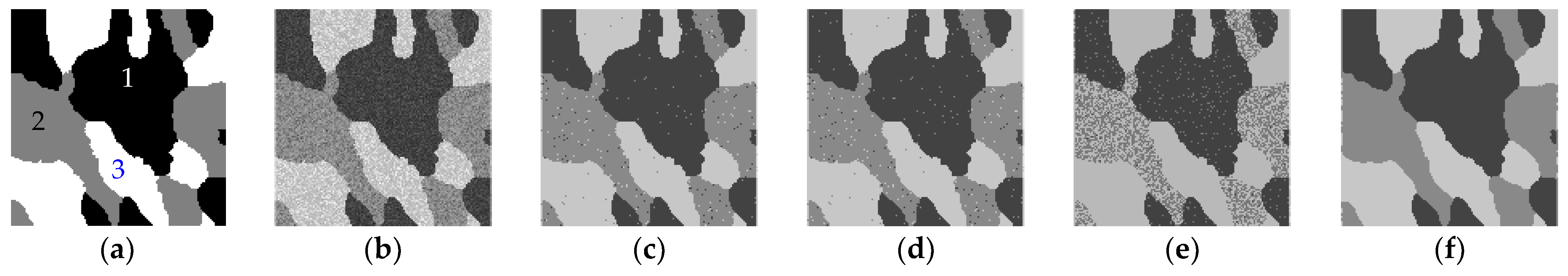
Figure 3a shows the template image with three homogeneous regions (1–3 are the labels of regions), and the simulated images generated using the parameters listed in Table 1 are shown in Figure 3b. Two sets of parameters were used in generating random values as pixel intensities for the three regions to simulate the spectral heterogeneity of remote sensing images. The FCM, GMM, SMM and HSMM algorithms were then used to segment the image, and the results are shown in Figure 3c–f.
In Figure 3c,d, FCM and GMM algorithms were able to segment each region, but some pixels were incorrectly segmented. The SMM algorithm (see Figure 3e) generated worse results than the FCM and GMM algorithms, with more pixels wrongly segmented, especially in region 2. In Figure 3f, the proposed HSMM algorithm was able to segment the regions accurately, with fewer pixels segmented erroneously.
Table 2 summarizes the accuracy results (i.e., product accuracy, overall accuracy and kappa coefficient) of the different segmentation algorithms for the simulated image (Figure 3). While the FCM and GMM algorithms produced good segmentation results with product accuracies above 95% in all three regions, some pixels were incorrectly segmented. For the SMM, due to the incorrect segmentation in region 2, the algorithm had the lowest product accuracy. The proposed HSMM algorithm was able to segment each region accurately, with product accuracies above 97% in all regions. In terms of overall accuracy, the HSMM algorithm had the highest value (98.92%), which was 1.11%, 1.31%, and 19.46% greater than the FCM, GMM, and SMM algorithms; for the kappa coefficient, the HSMM algorithm was 0.02, 0.02, and 0.27 higher than the other algorithms.
To test the modeling performance of the proposed algorithm, Figure 4a–c shows the histograms and the fitting curves of the simulated image using the proposed HSMM, where the black areas are the histograms of three regions and the red curves show the fitting curves of the HSMM algorithm. In Figure 4a,b, the histograms of regions 1 and 2 were asymmetric, while the histogram of region 3 was asymmetric and multimodal in Figure 4c. As shown in the figures, the components of HSMM can accurately fit the complex histograms. The component was defined using the weighted two Student’s t-distributions. It was flexible to fit the symmetrical histograms of regions 1 and 2, and the multimodal histogram of region 3. Further, the proposed HSMM can accurately build the statistical model of the simulated image.
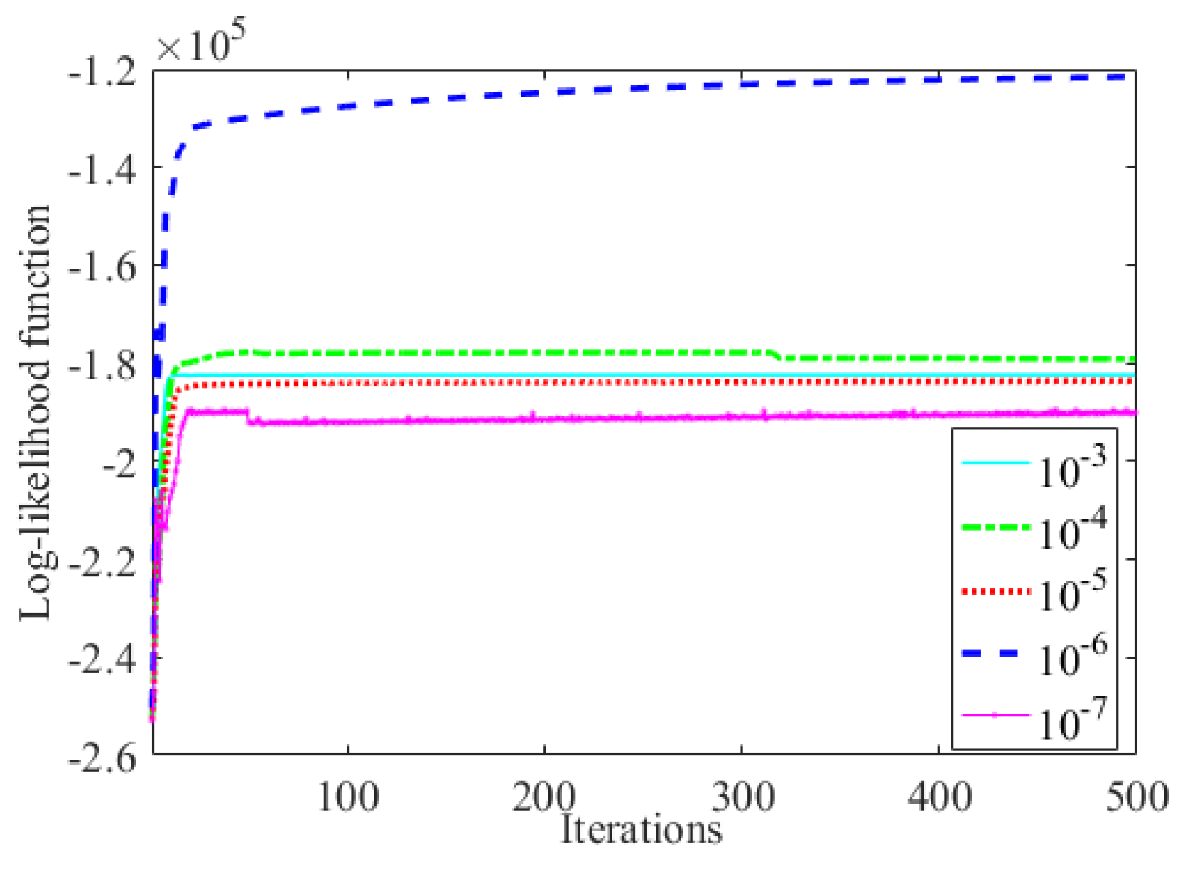
According to the principle of the gradient optimization method, the step length is able to affect the convergence of the log-likelihood function. For that, the log-likelihood functions with different step lengths are shown in Figure 5, aiming to analyse the influence of step length for the convergence. In Figure 5, the horizontal axis refers to the iteration count, the vertical axis indicates the log-likelihood function, and the curves correspond to the functions with different step lengths. As the number of iterations increased, the change in curve became increasingly smaller; at the 50th iteration, the functions almost remained unchanged. In addition, the functions converged to different values. When the step length was 10−6, the corresponding function was maximum. Based on the maximum log-likelihood function criterion, the step length 10−6 was selected as the empirical parameter for the subsequent segmentation experiments.

3.2. Synthetic Multispectral Image Segmentation

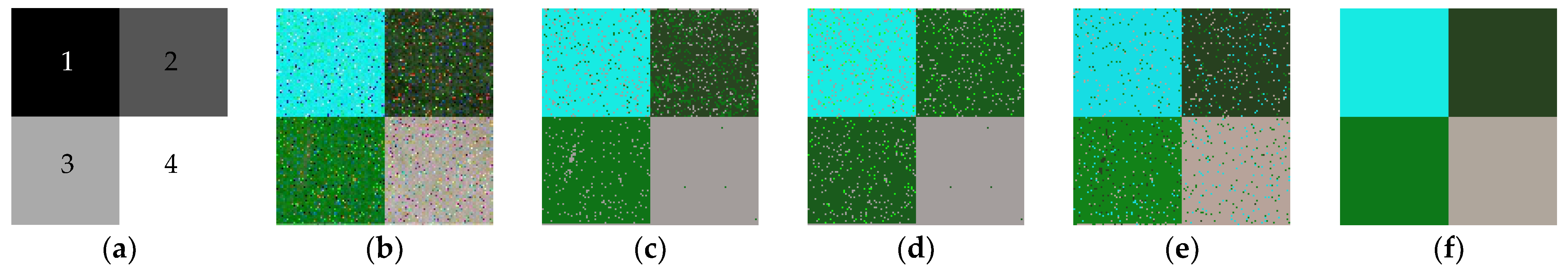
Figure 6 shows a synthetic multispectral image and its segmentation results. Figure 6a shows the template image having four homogeneous regions. In Figure 6b, the image was synthesized by intercepting four different regions (forest land, water, bare land, grassland) of multispectral image; 2% salt and pepper noise was randomly added to the synthetic image.
In the segmentation results, the FCM, GMM and SMM algorithms yielded lots of incorrect segmentation. The FCM algorithm generated segmentation errors, particularly in region 2 (see Figure 6c). The GMM algorithm was unable to segment regions 2 and 3 (see Figure 6d). The SMM algorithm was able to segment the regions but had incomplete segmentation and erroneous results in each region (see Figure 6e). In Figure 6f, the HSMM algorithm was able to accurately segment the region, with almost no incorrectly segmented results. The better result is because the proposed algorithm combined the HSMM and the correlation of local pixels for the reasonable use of spectral and spatial information. Hence, the proposed algorithm was robust to noise and obtained the optimal result.
Table 3 lists the segmentation accuracies (i.e., product accuracy, overall accuracy and kappa coefficient) of the various segmentation algorithms for the synthetic image (Figure 6). The FCM algorithm had product accuracy below 80% in one of the regions since it had incorrectly segmented in region 2. The GMM algorithm was unable to segment region 3, causing it to have a product accuracy of 0% for that region. The SMM algorithm was able to segment all regions, having product accuracies above 91%. The HSMM algorithm was able to accurately segment each region, and the product accuracy in all regions was 100%. In terms of overall accuracy, the HSMM algorithm was 10.39%, 29.01%, and 5.27% higher than the other algorithms; it also had a better kappa coefficient, which was 0.14, 0.36, and 0.09 higher than the other algorithms.

3.3. Remote Sensing Image Segmentation

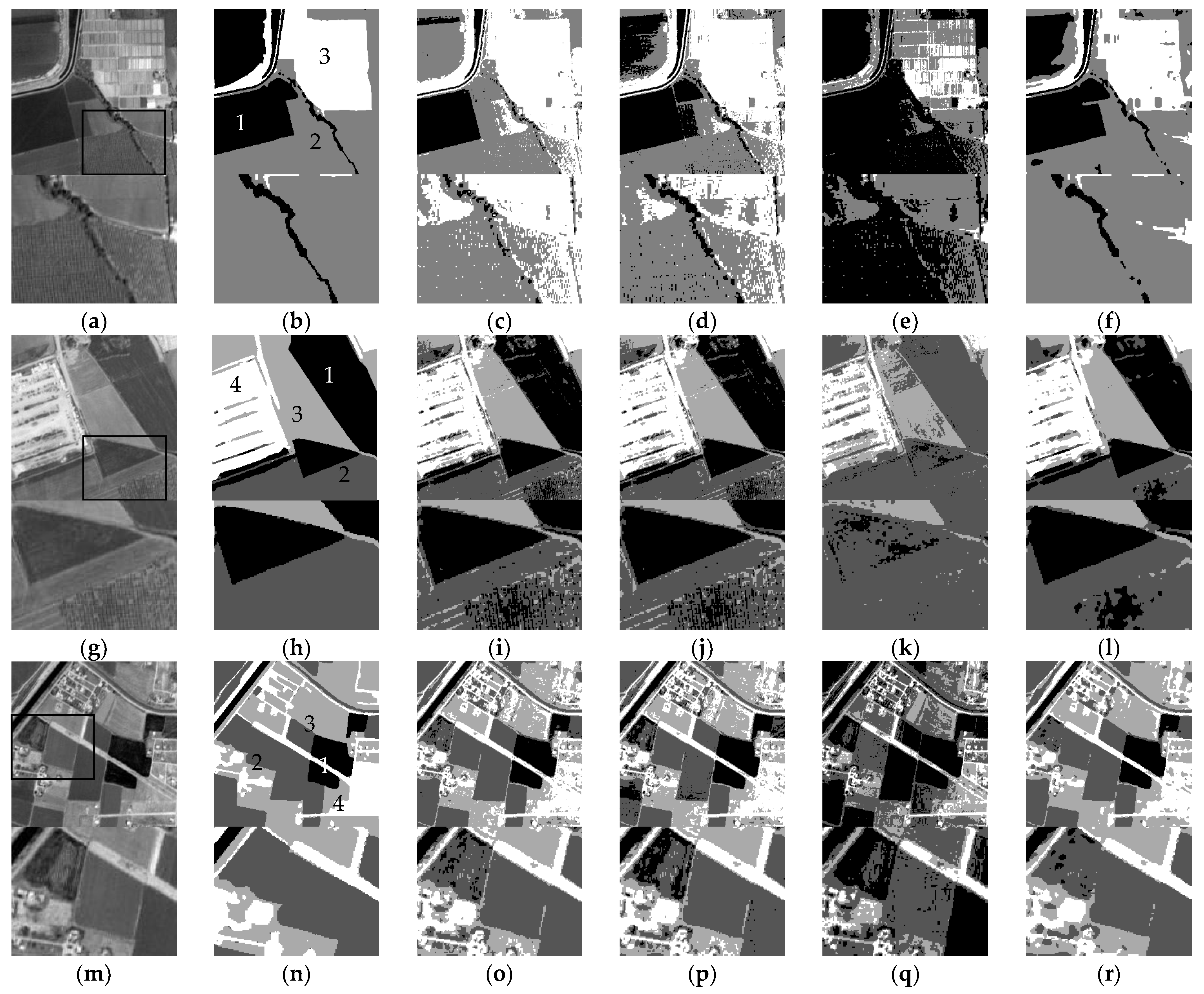
Various high-resolution panchromatic images were segmented (see Figure 7) to verify the effectiveness of the proposed HSMM algorithm. Figure 7a,g,m shows Cartosat1 images of farmland, bare land and buildings with a 2.5 m spatial resolution; the numbers of object regions were 3, 4, and 4. Standard segmentation (see Figure 7b,h,n) can be conducted using visual recognition for the quantitative evaluation, and the different regions can be labeled 1–4. In Figure 7c–f, the FCM and GMM algorithms were unable to segment region 1 and there were some wrongly segmented pixels in each region; the SMM algorithm could not segment each region, and its result was poor; the proposed algorithm better segmented each region, and there were a few incorrectly segmented pixels. In Figure 7i–l, the regions 1 and 3 were better segmented using the FCM and GMM algorithms, and the wrongly segmented pixels were mainly in region 2; the SMM was unable to segment regions 1 and 2, and there were many wrongly segmented pixels in regions 3 and 4; the proposed algorithm more accurately segmented each region and there were some wrong pixels in region 2. In Figure 7o–r, there were some incorrect pixels in the results of the FCM and GMM algorithms, and region 3 was segmented worse; the SMM algorithm was unable to segment regions 2 and 3; the result of the proposed algorithm was better than other algorithms, while there were some incorrect pixels in region 2. While the FCM and GMM algorithms considered the spatial correlation of local pixels, they were susceptible to spectral heterogeneity and obtained poor results, such as region 2 in Figure 7i,j. The SMM algorithm was unable to accurately segment each region and there was either over-segmentation or under-segmentation for farmland, such as region 1 of Figure 7e and region 2 of Figure 7q. Based on the spatial constraint, HSMM, the proposed algorithm, was able to reasonably utilize the spectral information, reduce spectral heterogeneity effects and obtain better results.
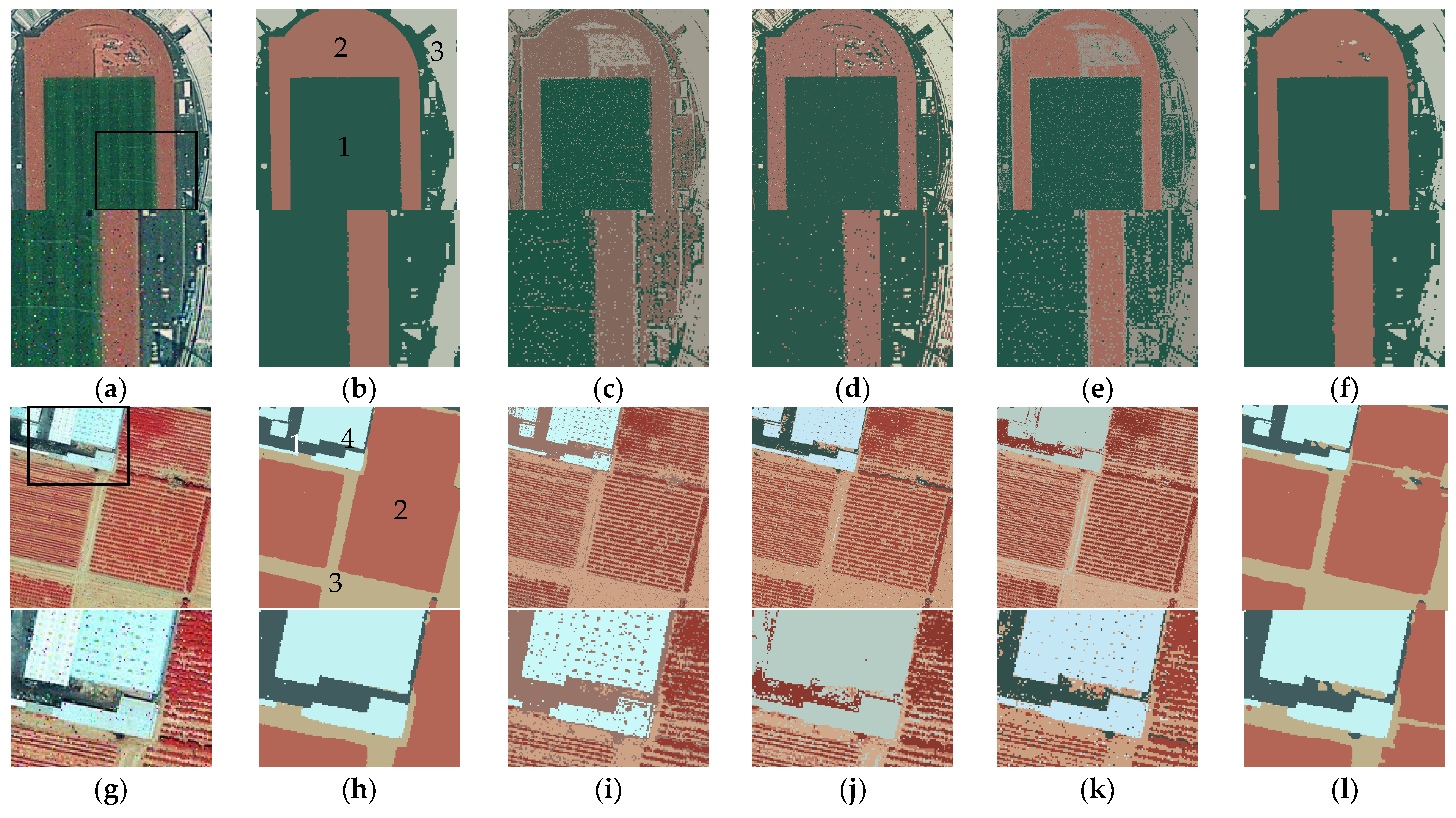
Figure 8a,g,m shows different high-resolution multispectral images with 2% salt and pepper noise to test the robustness of the proposed algorithm. Figure 8a has 0.5 m spatial resolution from GeoEye1 and includes building, an athletic track, and an area of artificial grass. Figure 8g is a 0.8 m spatial resolution image from Ikonos and includes buildings, farmland, and bare land. Figure 8m is a 0.5 m spatial resolution image from Worldview2 and includes buildings, roads, grassland and trees. The object regions in these figures were 3, 4, and 4. Visual recognition was used for generating the standard segmentation, and each region was labeled (1–4). In Figure 8c–f, the FCM and SMM algorithms were affected by noise, and some pixels in region 1 were wrongly segmented; there were less wrongly segmented pixels in Figure 8d using the GMM algorithm; a few pixels were wrongly segmented using the proposed algorithm, and the region was segmented accurately. The FCM, GMM, and SMM algorithms had difficulty segmenting region 2 with texture in Figure 8i–k, while the proposed algorithm introduced the spatial correlation to better segment each region in Figure 8l, especially texture region 2. The three comparative algorithms were unable to segment the road and grassland in Figure 8o–q, and shadow pixels were wrongly segmented. In contrast, the proposed HSMM algorithm was able to accurately segment road and grassland, and obtain a better result in Figure 8r; a few shadow pixels were erroneously segmented. The proposed algorithm utilized the spatial constraint HSMM to obtain the optimal segmentation. It was more robust to noise due to the correlation of local pixels, and avoided inaccurate segmentation of texture regions. Visually, the proposed HSMM algorithm generated better results than the other algorithms.
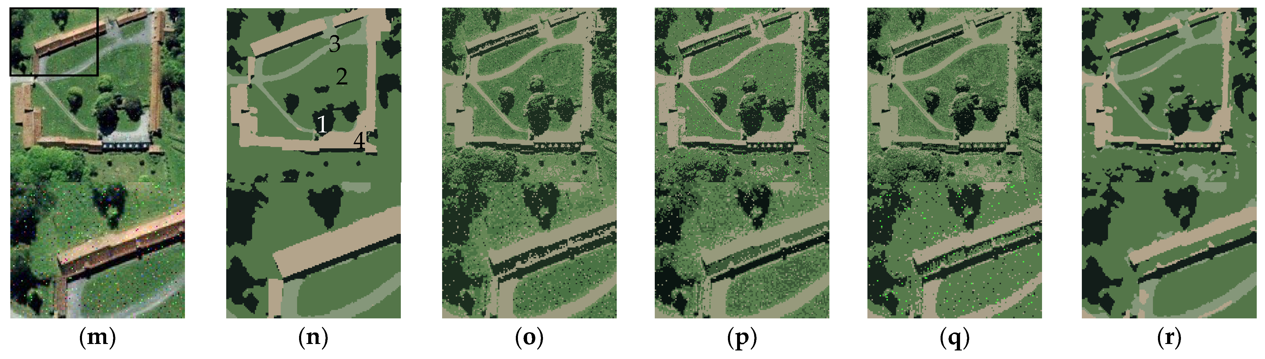
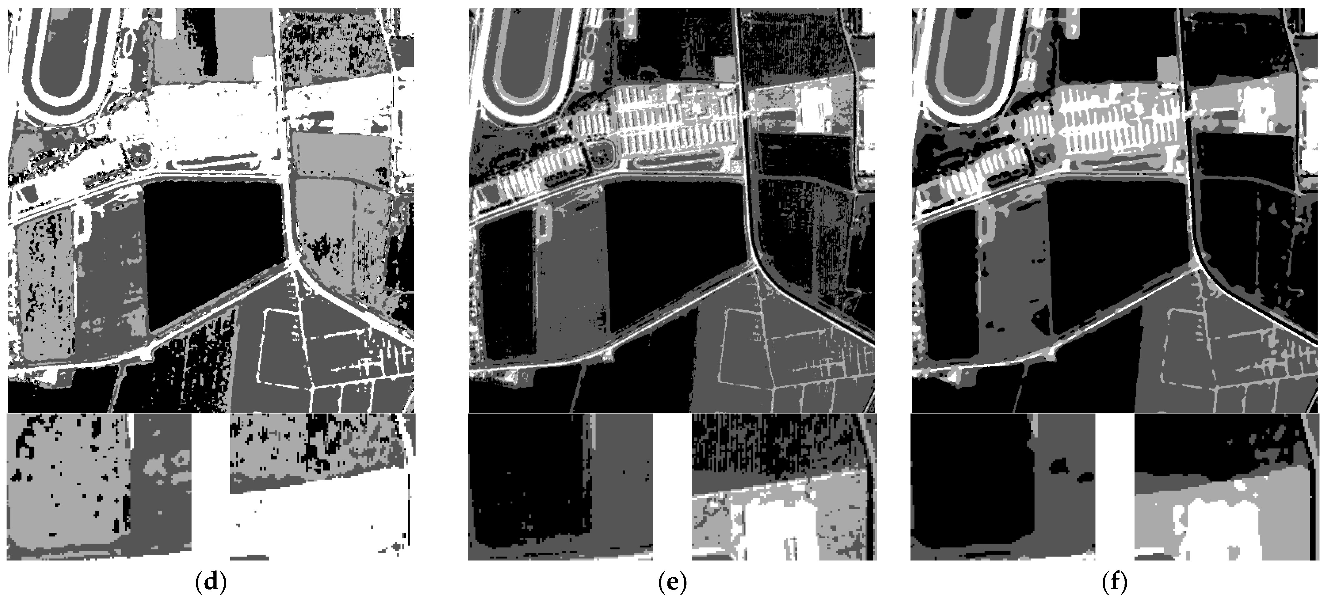
Figure 9 shows a large-scale panchromatic image with a high-resolution and its segmentation results. In Figure 9a, there is farmland, rest-arable land, bare land and a residential area, labeled as 1–4. The spectral heterogeneity is obvious in the image, especially in the farmland. There is spectral similarity between farmland and rest-arable land. In Figure 9c, the FCM algorithm was unable to segment each region. For example, many parts of region 1 were wrongly segmented into region 2, and it failed to segment regions 3 and 4. In Figure 9d, the GMM algorithm wrongly segmented parts of region 1 into region 3. Moreover, regions 3 and 4 were also unable to be segmented. The SMM algorithm obtained better result than the FCM and GMM algorithms in Figure 9e, while there were also wrongly segmented pixels in region 1. The proposed algorithm more accurately segmented each region, and less pixels were wrongly segmented in region 1. In general, the result of the proposed algorithm is optimal.
Table 4 summarizes the overall segmentation accuracies for the remote-sensing images (Figure 7, Figure 8 and Figure 9). The SMM algorithm had the lowest segmentation accuracy for the panchromatic images. The accuracy of the GMM algorithm was the lowest for the multispectral images except for the accuracy of segmenting Figure 8a. The FCM algorithm had the lowest accuracy of segmenting, Figure 9a. Compared with traditional segmentation algorithms, the proposed algorithm had better overall accuracy and its accuracy was greatly than 87%. Moreover, the average accuracy of the proposed algorithm was 26.08%, 25.73%, and 27.29% higher than the FCM, GMM, and SMM algorithms, respectively. Hence, the proposed algorithm obtained the best results for the remote sensing images.
Table 5 lists the segmentation times of the different algorithms to test the efficiency of the proposed HSMM algorithm. For remote sensing images in Figure 7 and Figure 8 with 256 × 256 pixels, the FCM, GMM, SMM, and HSMM algorithms had segmentation duration between 15 to 22 s, 14 to 22 s, 33 to 44 s, and 28 to 36 s, respectively. The scale of Figure 9a was 512 × 512 pixels, and its segmentation time was significantly more than other images for each algorithm. Hence, the larger the scale of the image, the more time it took to segment the image using the above algorithms. For the average time, the FCM and GMM algorithms were the least, the SMM algorithm was the most, and the proposed algorithm was better than the SMM algorithm. The FCM and GMM algorithms were able to deduce the formulas of parameters using minimum objective function and maximum likelihood estimation respectively, so they obtained segmentation results more efficiently. The SMM algorithm optimized the parameters using a gradient descent method and took much more time for convergence. The proposed algorithm combined the maximum likelihood estimation and gradient optimization method to solve parameters based on the simplified segmentation model. Hence, its time was better than the SMM algorithm and 9.2654 s less than the SMM algorithm on average.
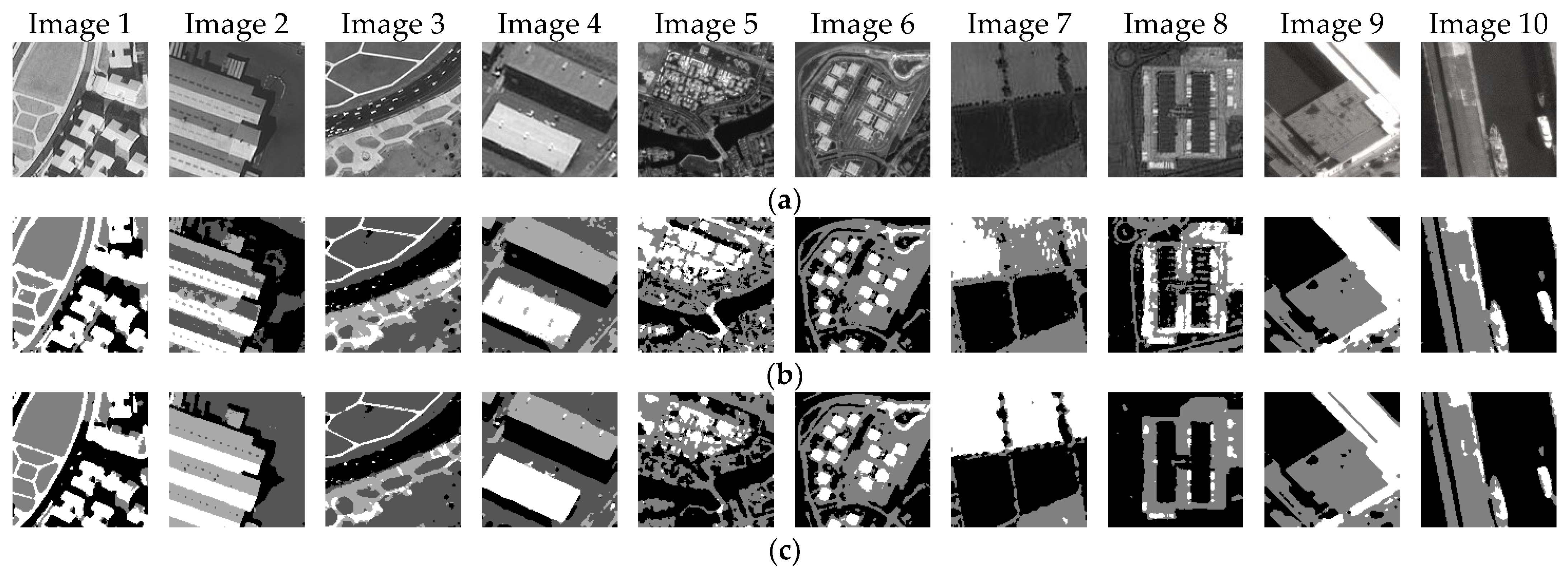
Figure 10 presents the segmentation results of 10 remote sensing images provided by the proposed algorithm and the Hierarchical GMM (HGMM)-based parameter optimization image segmentation algorithm (called HGMM algorithm). In Figure 10, images 1 and 2 are from EROS, images 3 and 4 are from Worldview1, images 5 and 6 are from SPOT5, images 7 and 8 are from Cartosat1, images 9 and 10 are from Pleiades1, respectively. For the image 1, the HGMM algorithm a better result, while the proposed algorithm was affected by the shadow and there were some wrongly segmented pixels. For the image 2, the HGMM algorithm was unable to segment the right region, while the proposed algorithm could better segment the image. For the images 7 and 8, the upper regions were incorrectly segmented using the HGMM algorithm, whereas the proposed algorithm was able to better segment each region and avoid the effect of spectral heterogeneity. For other images, the HGMM and the proposed algorithms accurately segmented them. Moreover, the results of the proposed algorithm were better than the HGMM algorithm in detail, such as the lower regions of images 3 and 5. Hence, the proposed algorithm is superior to the HGMM algorithm in segmentation performance.
Table 6 lists the segmentation time of the HGMM and HSMM algorithms for 10 remote sensing images. The time of the HGMM and HSMM algorithms was in the range of (1.66, 2.32) and (2.28, 2.97), respectively. They were affected by the number of classes. The greater the number of classes, the more segmentation time. Obviously, it taken more time to segment images 2, 3 and 4 than other images. Since the structure of Student’s t-distribution was more complex than Gaussian distribution and the parameter number of Student’s t-distribution was more than Gaussian distribution, the proposed algorithm took more time than the HGMM algorithm. For the average time, the proposed algorithm was 0.6693 s more than the HGMM algorithm.

4. Discussion

In the experiments of the first simulated image, under the qualitative and quantitative evaluation, the results show that the proposed algorithm obtained the best result. Firstly, the segmentation results show that the proposed algorithm can better segment each region and few pixels are wrongly segmented. However, the FCM, GMM and SMM algorithms incorrectly segmented the image. Its accuracy is higher than other algorithms. Secondly, the fitting result indicates the proposed algorithm is able to more accurately model complex distributions, such as asymmetric and multimodal distributions. The proposed algorithm exploits the HSMM using the weighted Student’s t-distributions as its component, and is suitable for modeling the complex characteristics of an image. Hence, it can effectively utilize spectral information to improve the segmentation performance. Moreover, the log-likelihood functions indicate that the functions are converging to different values given different step lengths. Based on maximum log-likelihood criterion, the step length corresponding to the maximum function is selected for the experiment, and it is set to 10−6 for a better performance.
The second experiment suggests that the proposed algorithm can also accurately segment a synthetic multispectral image with noises. The FCM, GMM, and SMM algorithms had difficulties reducing noise impacts, and their results are worse. The proposed algorithm introduces spatial information into the HSMM by defining the component weight with the correlation of neighborhood pixels. It greatly minimizes image noise effects and improves segmentation accuracy. Hence, the proposed algorithm is more robust to noise. Additionally, the simple structure of the component weight does not increase computation and complexity. However, the comparative algorithms are vulnerable to spectral heterogeneity and image noise.
In the experiments of the panchromatic images, the proposed algorithm obtained better results than the comparative algorithms. There were spectral heterogeneities in the high-resolution remote sensing image (Figure 7a,g,m), especially region 2 of Figure 7a, region 2 of Figure 7b, and region 3 of Figure 7m. While the FCM and GMM algorithms consider the spatial correlation of local pixels, they are still susceptible to spectral heterogeneity and there are incorrect pixels in their results. The SMM obtained poor result with over-segmentation. The proposed algorithm used the HSMM to accurately build the statistical model, optimizing the segmentation performance. Moreover, it introduced the correlation of local pixels to improve the robustness for the spectral heterogeneity. Compared with the segmentation accuracy, the proposed algorithm obtained the highest accuracy. It can obtain the optimal results for panchromatic image.
In the experiments involving the multispectral images, the proposed algorithm accurately segmented the images with noise. The added noise was randomly distributed in each image. The spectral heterogeneity is obvious in some regions of the images, such as the farmland of Figure 8g and the grassland of Figure 8m. Although the three comparative algorithms take the spatial information into account, they are still vulnerable to noise and spectral heterogeneity. For example, regions 2 (farmland) failed to be segmented in Figure 8i–k, and there were many pixels segmented wrongly in regions 2 (grassland) of Figure 8o–q. For the results of the proposed algorithm, each region was segmented more accurately, and few pixels were wrongly segmented. The advantage of the proposed algorithm is combining the HSMM and the component weight defined by the correlation of neighborhood pixels. The defined weight can effectively reduce the impact of noise. Especially, the HSMM is suitable for describing complex characteristics. For the segmentation accuracy, the proposed algorithm was higher than the other algorithms. Hence, it had the ability to segment the image with noise, and obtain the best result.
In the experiments using a large scale image, the spectral heterogeneity in region 1 and the spectral similarity between regions 1 and 2 were obvious. The proposed algorithm obtained a better result than the other algorithms. Although the comparative algorithm used the spatial correlation to improve performance, there were many regions incorrectly segmented in Figure 9c–e. The pixels of region 1 were wrongly segmented into other regions due to the heterogeneity of the pixels; regions 2 and 3 were not segmented due to the spectral similarity. The proposed algorithm can better segment the image. On the one hand, it can flexibly model the statistical characteristic of the spectrum to make full use of spectral information; on the other hand, it applies a spatial correlation to improve the robustness.
The segmentation time shows that the proposed algorithm has a higher efficiency. The segmentation time of FCM, GMM, SMM and HSMM algorithms is affected by the image scale. The larger the scale of the image, the more time is taken to segment the image using the above algorithms. Since the FCM and GMM algorithms deduce the parameter formulas and the formulas are simple to calculate, they have the highest segmentation efficiency. The SMM algorithm optimizes its parameters by calculating their gradients, and it takes more time for convergence. The proposed algorithm has a higher efficiency than the SMM algorithm, since it simplifies the segmentation model and optimizes the parameter solution, combining the maximum likelihood estimation and gradient optimization method. Moreover, the proposed algorithm employs an adaptive smoothing coefficient to avoid over-segmentation or under-segmentation caused by artificially setting the coefficient. While its efficiency is not better than FCM and GMM algorithms, the proposed algorithm has optimal results with higher efficiency.
The experiments using the HGMM and proposed HSMM algorithms on 10 remote sensing images indicate that the HGMM and HSMM algorithms both accurately segment remote sensing images. The proposed algorithm can better segment image in detail and reduce the effect of spectral heterogeneity. This is because Student’s t-distribution is more robust than Gaussian distribution. Moreover, the HGMM has better efficiency than the proposed algorithm, due to the complex structure and the larger number of parameters of Student’s t-distribution. The proposed algorithm can obtain the optimal segmentation result.

5. Conclusions

To better segment high-resolution remote sensing images, an HSMM-based image segmentation algorithm with spatial constraints is proposed. Experimental results show that the HSMM algorithm can accurately model asymmetric, heavy-tailed, and bimodal distributions. Compared with traditional segmentation algorithms, the proposed HSMM algorithm effectively overcomes noise effects, providing higher efficiency and better precision segmentation results for high-resolution remote sensing images. The proposed algorithm is more suitable for panchromatic and multispectral remote sensing image segmentation. The limitation of the proposed algorithm is the number of components being fixed. How to adaptively determine the number of components is a key problem and difficulty in image segmentation. There is no universal solution. The Reversible Jump Markov Chain Monte Carlo (RJMCMC) method can solve the number of components and parameters. However, sampling of the method requires too much time. The poor efficiency of RJMCMC should be improved as the result of future research.

Author Contributions

Conceptualization, X.S.; methodology, X.S. and Y.L.; software, X.S. and Y.W.; validation, X.S.; formal analysis, X.S., Y.W., Y.L. and S.D; writing—review and editing, X.S.; funding acquisition, X.S., Y.W. and S.D. All authors have read and agreed to the published version of the manuscript.

Funding

This research was funded by Guangxi Natural Science Foundation of China, grant number 2022GXNSFBA035567 and 2020GXNSFBA297096, Natural Science Foundation of China, grant number 42061059.

Data Availability Statement

Not applicable.

Conflicts of Interest

The authors declare no conflict of interest.

References

  1. Zhang, X.L.; Xiao, P.F.; Feng, X.Z.; Yuan, M. Separate segmentation of multi-temporal high-resolution remote sensing images for object-based change detection in urban area. Remote Sens. Environ. 2017, 201, 243–255. [Google Scholar] [CrossRef]
  2. Kotaridis, I.; Lazaridou, M. Remote sensing image segmentation advances: A meta-analysis. ISPRS J. Photogramm. Remote Sens. 2021, 173, 309–322. [Google Scholar] [CrossRef]
  3. Hossain, M.D.; Chen, D.M. Segmentation for object-based image analysis (OBIA): A review of algorithms and challenges from remote sensing perspective. ISPRS J. Photogramm. Remote Sens. 2019, 150, 115–134. [Google Scholar]
  4. Shen, Y.; Chen, J.Y.; Xiao, L.; Pan, D.L. Optimizing multiscale segmentation with local spectral heterogeneity measure for high resolution remote sensing images. ISPRS J. Photogramm. Remote Sens. 2019, 157, 13–25. [Google Scholar] [CrossRef]
  5. Wang, M.; Dong, Z.P.; Cheng, Y.F.; Li, D. Optimal segmentation of high-resolution remote sensing image by combining superpixels with the minimum spanning tree. IEEE Trans. Geosci. Remote Sens. 2018, 56, 228–238. [Google Scholar] [CrossRef]
  6. Golpardaz, M.; Helfroush, M.S.; Danyali, H. A new conditional random field based on mixture of generalized Gaussian model for synthetic aperture radar image segmentation. Int. J. Remote Sens. 2021, 42, 4743–4761. [Google Scholar] [CrossRef]
  7. Chatzis, S.P. A fuzzy clustering approach toward hidden Markov random field models for enhanced spatially constrained image segmentation. IEEE Trans. Fuzzy Syst. 2008, 16, 1351–1361. [Google Scholar] [CrossRef]
  8. Tong, X.Y.; Xia, G.S.; Lu, Q.K.; Shen, H.F. Land-cover classification with high-resolution remote sensing images using transferable deep models. Remote Sens. Environ. 2020, 237, 111322. [Google Scholar] [CrossRef]
  9. Yang, J.; He, Y.H.; Caspersen, J. Region merging using local spectral angle thresholds: A more accurate method for hybrid segmentation of remote sensing images. Remote Sens. Environ. 2017, 190, 137–148. [Google Scholar] [CrossRef]
  10. Jin, X.L.; Niu, P.W.; Liu, L.F. A GMM-based segmentation method for the detection of water surface floats. IEEE Access 2019, 7, 119018–119025. [Google Scholar] [CrossRef]
  11. Wang, D. Efficient level-set segmentation model driven by the local GMM and split Bregman method. IET Image Process. 2019, 13, 761–770. [Google Scholar] [CrossRef]
  12. Shi, X.; Li, Y.; Zhao, Q.H. Flexible hierarchical Gaussian mixture model for high-resolution remote sensing image segmentation. Remote Sens. 2020, 12, 1219. [Google Scholar] [CrossRef]
  13. Grinias, I.; Panagiotakis, C.; Tziritas, G. MRF-based segmentation and unsupervised classification for building and road detection in peri-urban areas of high-resolution satellite images. ISPRS J. Photogramm. Remote Sens. 2016, 122, 145–166. [Google Scholar] [CrossRef]
  14. Yin, S.L.; Zhang, Y.; Karim, S. Large scale remote sensing image segmentation based on fuzzy region competition and Gaussian mixture model. IEEE Access 2018, 6, 26069–26080. [Google Scholar] [CrossRef]
  15. Nguyen, T.M.; Wu, Q.M.J. Fast and robust spatially constrained Gaussian mixture model for image segmentation. IEEE Trans. Circuits Syst. Video Technol. 2013, 23, 621–635. [Google Scholar] [CrossRef]
  16. Sammaknejad, N.; Zhao, Y.J.; Huang, B. A review of the expectation maximization algorithm in data-driven process identification. J. Process Control 2018, 73, 123–136. [Google Scholar] [CrossRef]
  17. Wang, P.; Zhu, H.; Ling, X. Content-based superpixel matching using spatially constrained Student’s-t mixture model and scale-invariant key-superpixel. IEEE Access 2020, 8, 31198–31213. [Google Scholar] [CrossRef]
  18. Sun, J.Y.; Zhou, A.M.; Keates, S.; Liao, S.B. Simultaneous Bayesian clustering and feature selection through Student’s t mixtures model. IEEE Trans. Neural Netw. Learn. Syst. 2018, 29, 1187–1199. [Google Scholar] [CrossRef]
  19. Yang, Y.; Han, S.D.; Wang, T.J.; Tao, W.B. Multilayer graph cuts based unsupervised color–texture image segmentation using multivariate mixed Student’s t-distribution and regional credibility merging. Pattern Recognit. 2013, 46, 1101–1124. [Google Scholar] [CrossRef]
  20. Nguyen, T.M.; Wu, Q.M.J. Robust Student’s-t mixture model with spatial constraints and its application in medical image segmentation. IEEE Trans. Med. Imaging 2012, 31, 103–116. [Google Scholar] [CrossRef]
  21. Gao, G.; Wen, C.; Wang, H. Fast and robust image segmentation with active contours and Student’s-t mixture model. Pattern Recognit. 2017, 63, 71–86. [Google Scholar] [CrossRef]
  22. Xiong, T.; Zhang, Y.; Lei, Z. Grayscale image segmentation by spatially variant mixture model with Student’s t-distribution. Multimed. Tools Appl. 2014, 72, 167–189. [Google Scholar] [CrossRef]
  23. Kong, L.C.; Zhang, H.; Zheng, Y.H.; Chen, Y.J. Image segmentation using a hierarchical Student’s-t mixture model. IET Image Process. 2017, 11, 1094–1102. [Google Scholar] [CrossRef]
  24. Zhang, H.; Wu, Q.M.J.; Nguyen, T.M.; Sun, X. Synthetic aperture radar image segmentation by modified Student’s-t mixture model. IEEE Trans. Geosci. Remote Sens. 2014, 52, 4391–4403. [Google Scholar] [CrossRef]
  25. Banerjee, A.; Maji, P. Spatially constrained Student’s t-distribution based mixture model for robust image segmentation. J. Math. Imaging Vis. 2018, 60, 355–381. [Google Scholar] [CrossRef]
  26. Shao, W.M.; Ge, Z.Q.; Song, Z.H.; Wang, J.B. Semisupervised robust modeling of multimode industrial processes for quality variable prediction based on Student’s-t mixture model. IEEE Trans. Industr. Inform. 2020, 16, 2965–2976. [Google Scholar] [CrossRef]
  27. Wei, X.; Li, C.G. The Student’s -hidden Markov model with truncated stick-breaking priors. IEEE Signal Process. Lett. 2011, 18, 355–358. [Google Scholar]
  28. Zheng, Y.H.; Jeon, B.; Sun, L.; Zhang, J.W.; Zhang, H. Student’s t-hidden Markov model for unsupervised learning using localized feature selection. IEEE Trans. Circuits Syst. for Video Technol. 2018, 28, 2586–2598. [Google Scholar] [CrossRef]
  29. Zhu, H.; Xie, Q. A multiphase level set formulation for image segmentation using a MRF-based nonsymmetric Student’s-t mixture model. Signal Image Video Process. 2018, 12, 1577–1585. [Google Scholar] [CrossRef]
Figure 1. The schematic diagram of the segmentation algorithm using the spatial constraint HSMM.
Remotesensing 15 00828 g001
Figure 2. The components of SMM and HSMM. (a) The components of SMM under varying degrees of freedom (v is set to 10, 2, 1, and 0.5). (b) The HGMM components with weights (0.8, 0.2). (c) The HGMM components with weights (0.3, 0.7). (d) The HGMM components with weights (0.5, 0.5).
Remotesensing 15 00828 g002
Figure 3. The segmentation experiment of the simulated image. (a) the template image, and 1–3 are the labels of regions, (b) the simulated image, (c) FCM algorithm, (d) GMM algorithm, (e) SMM algorithm, (f) HSMM algorithm.
Remotesensing 15 00828 g003
Figure 4. The fitting results of the histogram of the simulated image. (ac) regions 1–3.
Remotesensing 15 00828 g004
Figure 5. Likelihood function curve with different steps.
Remotesensing 15 00828 g005
Figure 6. The segmentation experiment of the multispectral synthetic image. (a) the template image, and 1–4 are the labels of regions, (b) the noise multispectral synthetic image, (c) FCM algorithm, (d) GMM algorithm, (e) SMM algorithm, (f) HSMM algorithm.
Remotesensing 15 00828 g006
Figure 7. High-resolution panchromatic images and their segmentation results. (a,g,m) high-resolution panchromatic images with noise, and the region in the black square is highlighted, (b,h,n) standard segmentation images, and 1–4 are the labels of regions, (c,i,o) FCM algorithm, (d,j,p) GMM algorithm, (e,k,q) SMM algorithm, (f,l,r) HSMM algorithm.
Remotesensing 15 00828 g007
Figure 8. High-resolution multispectral images and their segmentation results. (a,g,m) high-resolution multispectral images with noise, and the region in the black square is highlighted, (b,h,n) standard segmentation images, and 1–4 are the labels of regions, (c,i,o) FCM algorithm, (d,j,p) GMM algorithm, (e,k,q) SMM algorithm, (f,l,r) HSMM algorithm.
Remotesensing 15 00828 g008aRemotesensing 15 00828 g008b
Figure 9. Large scale panchromatic image with high-resolution and its segmentation results. (a) high-resolution panchromatic images, and the region in the black square is highlighted, (b) standard segmentation images, and 1–4 are the labels of regions, (c) FCM algorithm, (d) GMM algorithm, (e) SMM algorithm, (f) HSMM algorithm.
Remotesensing 15 00828 g009aRemotesensing 15 00828 g009b
Figure 10. High-resolution remote sensing images and their segmentation results. (a) high-resolution remote sensing images, (b) HGMM-GD algorithm, (c) HSMM algorithm.
Remotesensing 15 00828 g010
Table 1. The parameters of generating the simulated image.
ParameterRegion 1 (k = 1)Region 2 (k = 2)Region 3 (k = 3)
m = 1m = 2m = 1m = 2m = 1m = 2
wkm0.40.60.40.60.40.6
μkm6078130150190220
σkm78189810
Table 2. The segmentation accuracy of the simulated image.
AlgorithmProduct AccuracyOverall AccuracyKappa Coefficient
Region 1Region 2Region 3
FCM algorithm98.1695.0099.7697.730.96
GMM algorithm97.8695.0299.7397.610.96
SMM algorithm90.4747.0996.4979.460.71
HSMM algorithm97.8998.81100.0098.920.98
Table 3. The segmentation accuracy of the noise multispectral synthetic image.
AlgorithmProduct AccuracyOverall AccuracyKappa Coefficient
Region 1Region 2Region 3Region 4
FCM algorithm90.1475.1293.2699.9089.610.86
GMM algorithm89.8994.140.00100.0070.990.64
SMM algorithm95.0491.9991.6394.7393.350.91
HSMM algorithm100.00100.00100.00100.00100.001.00
Table 4. The segmentation accuracy of remote sensing images.
AlgorithmFigure 7aFigure 7gFigure 7mFigure 8aFigure 8gFigure 8mFigure 9aAverage
FCM69.0684.7982.8277.4356.1853.5833.9965.40
GMM82.6484.6480.7183.3231.4143.3354.1965.75
SMM53.8451.7238.7191.1964.6269.3879.8864.19
HSMM91.6388.2589.4498.5397.5287.4487.5291.48
Table 5. Efficiency performance of the different segmentation algorithms.
AlgorithmFigure 7aFigure 7gFigure 7mFigure 8aFigure 8gFigure 8mFigure 9aAverage
FCM15.602718.938819.865416.797621.022319.898845.739622.5521
GMM20.984416.790618.832814.175920.478721.846042.736122.2635
SMM33.611635.682438.733637.985043.218443.687582.084345.0004
HSMM28.524829.488430.082429.599733.871835.307763.270735.7350
Table 6. Efficiency performance of the HGMM-GD and HSMM algorithms.
AlgorithmImage 1Image 2Image 3Image 4Image 5Image 6Image 7Image 8Image 9Image 10Average
HGMM1.71502.21702.28192.31921.68201.71671.71261.68491.66851.66061.8659
HSMM2.39062.95982.95292.96872.36692.37082.37392.38192.28972.29842.5352
Disclaimer/Publisher’s Note: The statements, opinions and data contained in all publications are solely those of the individual author(s) and contributor(s) and not of MDPI and/or the editor(s). MDPI and/or the editor(s) disclaim responsibility for any injury to people or property resulting from any ideas, methods, instructions or products referred to in the content.

