Few-Shot Remote Sensing Image Scene Classification Based on Metric Learning and Local Descriptors

Abstract

Scene classification is a critical technology to solve the challenges of image search and image recognition. It has become an indispensable and challenging research topic in the field of remote sensing. At present, most scene classifications are solved by deep neural networks. However, existing methods require large-scale training samples and are not suitable for actual scenarios with only a few samples. For this reason, a framework based on metric learning and local descriptors (MLLD) is proposed to enhance the classification effect of remote sensing scenes on the basis of few-shot. Specifically, MLLD adopts task-level training that is carried out through meta-learning, and meta-knowledge is learned to improve the model’s ability to recognize different categories. Moreover, Manifold Mixup is introduced by MLLD as a feature processor for the hidden layer of deep neural networks to increase the low confidence space for smoother decision boundaries and simpler hidden layer representations. In the end, a learnable metric is introduced; the nearest category of the image is matched by measuring the similarity of local descriptors. Experiments are conducted on three public datasets: UC Merced, WHU-RS19, and NWPU-RESISC45. Experimental results show that the proposed scene classification method can achieve the most advanced results on limited datasets.

1. Introduction

Scene classification [1] is to judge the category of an image according to the scene content. Remote sensing (RS) scene classification [2,3] refers to the fact that remote sensing scene images are assigned specific labels and classified by some algorithm. It plays an irreplaceable role in crop yield estimation, disaster prevention, resource protection, and land planning and utilization. So far, with the extensive application of deep learning [4,5] in RS scene classification, great success has been achieved, most of the work of RS scene classification is based on large-scale remote sensing data sets, and more than thousands of images of each type are used to fit the neural network model. However, the process of labeling a large-scale dataset is very complex and labor-intensive. In contrast, few-shot learning [6,7] does not require a lot of labeled data. It tries to imitate human ability, where classification systems can learn to classify based on a small quantity of labeled images (few shots). One-shot learning [8] is included in few-shot learning, where each class of one-shot learning contains one sample. In addition, zero-shot learning [9] refers to the recognition of new things that have never been seen by computers, which is more demanding than few-shot learning.

Since deep learning abandons the traditional manual learning features, RS scene classification based on deep learning is of great significance [10,11,12,13]. Recently, Zhai et al. [14] proposed a useful model for lifelong learning that extracts prior knowledge by learning the ability of the classifier to achieve rapid generalization to new data sets. For the purpose of achieving the purpose of the model, which is to learn the global features of an image, Zhang et al. [15] introduced the remote sensing transformer (TRS) into RS scene classification to capture long-range dependency. For the benefit of mining the semantic features of different categories through the global features of RS images, Tang et al. [16] constructed RS images by spatial rotation on the basis of previous studies to capture more useful information and reduce the possibility of misclassification by improving the discrimination of features.

Few-shot learning is used to classify RS scenes with insufficient labeled data, which can solve the defects of the above methods and improve the interpretation performance [17,18,19,20,21,22]. For the sake of solving the disadvantage that RS images lack the ability to learn more judgmental features and reliable metrics, Li et al. [23] proposed an adaptive distance-based matcher to ameliorate the classification efficiency, called DLA-MatchNet. Sample-based training methods exist in most experiments and can achieve better results, but the probability of fitting individual samples will be greatly increased. By summarizing the previous methods, Li et al. [24] concluded that different tasks should be trained to extract features instead of samples and proposed an extremely reliable method called RS-MetaNet. The effectiveness of the prototype is ignored by most existing prototype-based few-shot learning, and directly calculating the prototype from the support sample will lead to a decrease in the accuracy of subsequent inferences. In view of the above issues, Cheng et al. [25] proposed a combination of the SC method without adding any learnable parameters and the IC method to increase the prediction accuracy. The addition of these two Siamese prototypes can extract more representative feature information for RS scene classification. In order to address the drawback that insufficient labeled samples make it difficult to extract categorical features, Zeng et al. [26] proposed an iterative looping architecture (IDLN) to improve classification performance. Due to the problem of sample quantity, the learning ability of the model is markedly reduced. In order to identify the classification boundary that depends on the sample deviation, the distance between different categories is widened and the data of the same category is polymerized. Cui et al. [27] proposed a framework called meta kernel networks (MKNs). For automatic modulation classification, which requires a large number of labeled samples, Che et al. [28] designed two feature extraction networks, which correspond to spatial and temporal feature spaces, respectively. The classification results of the two feature spaces are fused. In addition, a new mixed loss function is designed to expand the distance between classes. Furthermore, some graph-based methods [29,30] have also achieved advanced results in the field of remote sensing. To address the problems of noise influence and insufficient labeled training samples in hyperspectral classification. Zhang et al. [31] proposed a mechanism for automatically exploring receptive fields and learning the importance of different neighborhoods. When the node is updated, the local information of the node is not discarded. It is difficult to identify the global information of the graph for the existing graph-based methods. Ding et al. [32] proposed a semi-supervised network that flexibly aggregates graph nodes between data and captures deeper relationships based on the relationship between the obtained contexts.

Meta-learning is often used to solve few-shot problems because of its self-learning ability and strong generalization performance. Meta-learning research is currently divided into three independent methods: metric-based methods, optimization-based methods, and model-based methods. Among them, model-based meta-learning has made the most progress. At present, the best experimental accuracy results come from the subsequent improvement of Model-Agnostic Meta-Learning [33] (MAML) algorithms in this direction. This direction has also become the backbone of the meta-learning field. In data augmentation-based methods, Li et al. write the features of a set of labeled images (support sets) into memory and extract them from the memory while performing inference, making full use of the knowledge in the set, called MatchingNet [34]. In the metric-based methods, the classical networks include relational networks [35], prototype networks [6], etc. According to these two models, many novel meta-learning models have been developed.

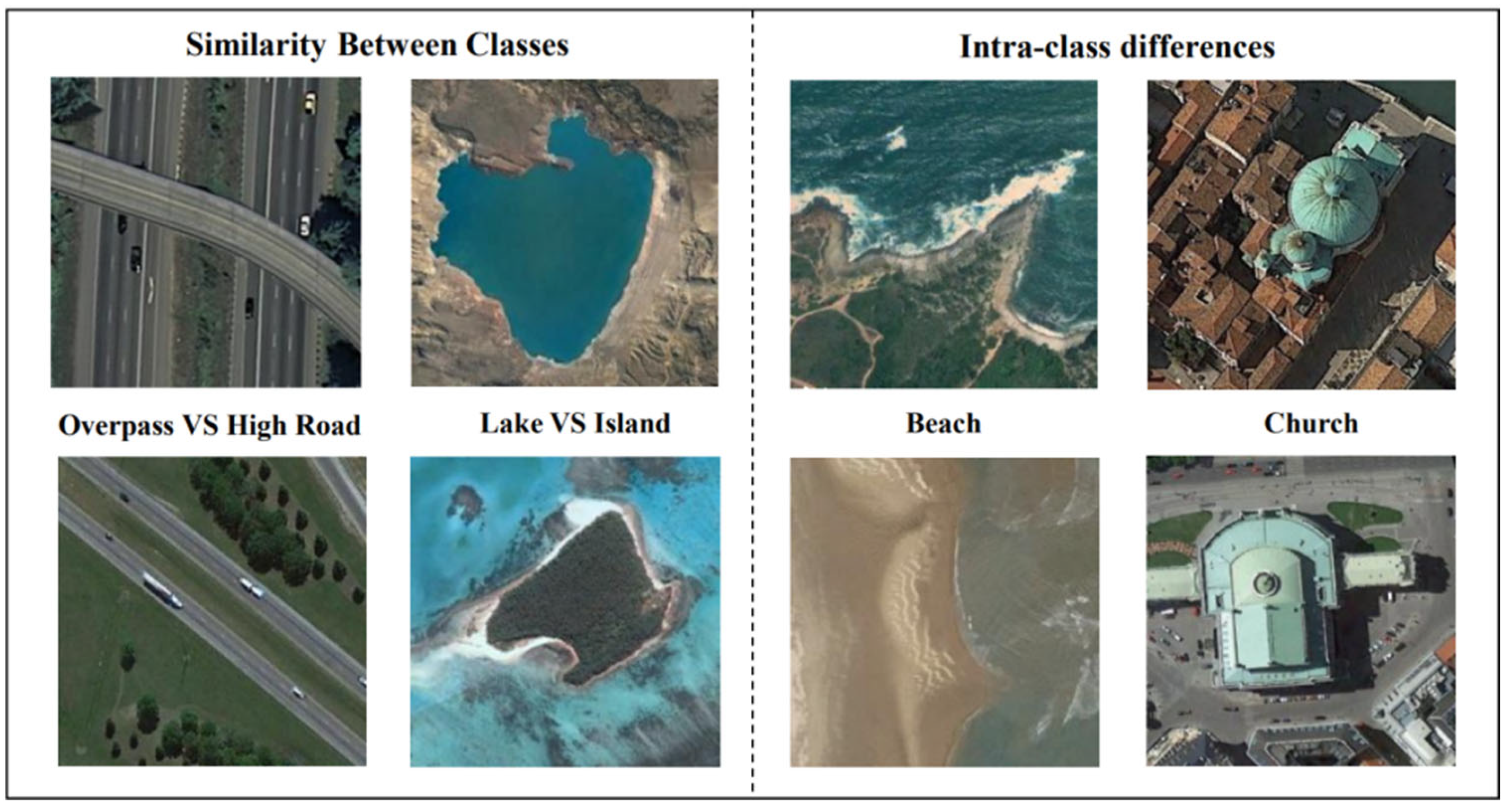
The methods mentioned above mainly focus on sample-level features for few-shot RS scene classification, resulting in learned features that easily overfit individual samples, and most use metrics based on image-level features. Meanwhile, the problem of fuzzy hidden layer representation and decision boundary in neural networks is ignored, so accurate feature representation is difficult to learn. In addition, RS images have large differences with natural images due to different shooting content and shooting methods, such as aerial photos and satellite photos. Therefore, few-shot learning needs to overcome the influence of indistinguishable features and unrelated backgrounds between categories caused by remote sensing images due to shooting methods, as indicated in Figure 1. For the above-mentioned problems, few-shot learning should be organized based on tasks rather than image-level. At the same time, the diversity of feature vectors should be increased to learn accurate feature representation. In addition, image-to-class metrics based on local descriptors are adopted for final classification.

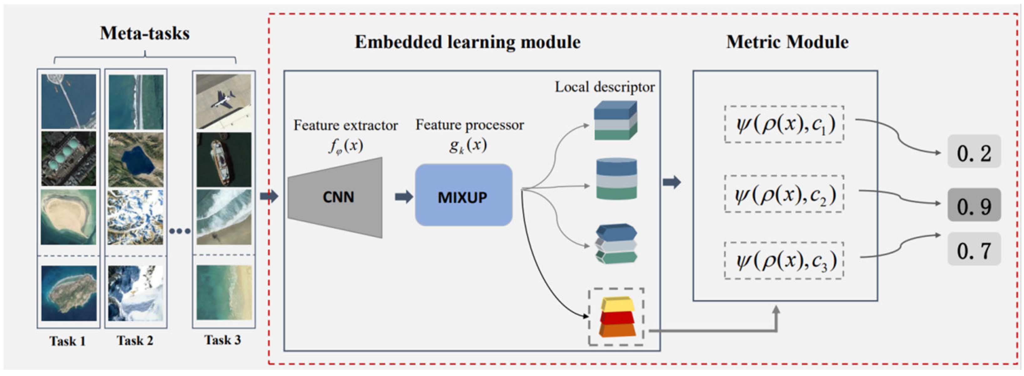
Aiming at the challenges brought by the above problems, a few-shot RS scene classification method based on metric learning and local descriptors is proposed, called MLLD, which not only has the capacity to increase the classification accuracy of RS scene images with fewer labels but also addresses the aforementioned issues. The overall framework of the model consists of Meta-tasks Module, Deep Embedded Learning Module, and Metric Module. Firstly, the meta-task module has the ability to simulate human learning, learn various knowledge through different meta-tasks, and finally achieve the purpose of learning to classify rare samples. The performance of meta-learning on each task increases with experience and the number of tasks; that is, the efficiency of the model is gradually improved by learning multiple tasks. The Meta-tasks Module to learn task-based metrics can be better extended to invisible test tasks. Secondly, the Embedded Learning Module extracts and fuses features to increase the diversity of feature vectors, including the part of extracting and processing features. The existence of hidden layer representation and decision boundary ambiguity in neural networks leads to a lot of irrelevant noise being learned during model training, which affects the adaptability of the model to fresh samples and reduces the classification accuracy of the test data. Our model comes up with solutions to these challenges, the feature processor uses Manifold Mixup [36] to apply to the hidden layer of deep neural networks; that is, the model is required to satisfy linear constraints on the operation at the feature level, and this constraint is used to regularize the model. Finally, the processed feature vector is divided into local descriptors. The last layer of measurement image-level features is replaced by measuring image-to-class local descriptors. According to local invariant features, this method can achieve breakthrough results. At the same time, using local descriptors in few-shot can reduce the computation of searching for the nearest neighbors from local descriptors in a large sample.

2. Proposed Method

The focus of this paper is to solve the two major challenges of RS scene classification: (1) The lack of labeled samples and the nature of neural networks make it difficult for the model to learn accurate feature representations. (2) Few-shot RS scene classification needs to perform classification tasks under the influence of small distances between different categories and larger intra-class variance. In addition, irrelevant background information will be confused with valid content, which can affect classification accuracy. The proposed model is shown in Figure 2. Firstly, the Meta-tasks Module improves the problem-solving ability of the model by learning meta-knowledge from multiple tasks through meta-training, which is an extremely effective method to solve few-shot tasks. Second, the Embedded Learning Module not only extract features but also enrich the diversity of features. Finally, the local descriptor is used by the Metric Module to calculate the similarity between the image and category.

2.1. Meta Task Module

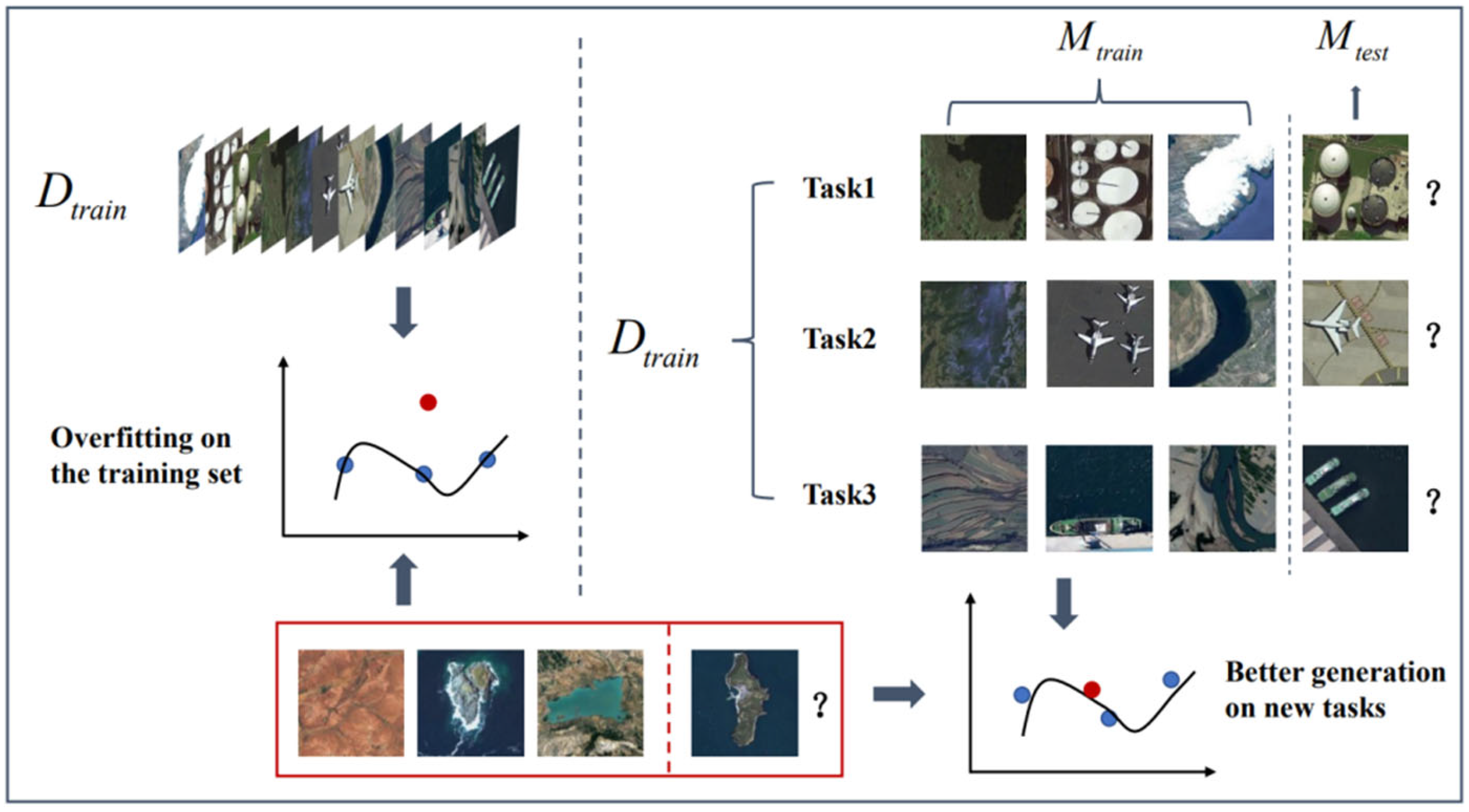
Deep learning essentially uses thousands of pieces of data to train the model and then gradually updates the model parameters in the opposite direction of loss gradient descent, so that the accuracy of classification is improved until the optimal model is learned. General deep learning only considers the information between samples, while the relationship between few-shot tasks is ignored, which leads to the phenomenon of fitting to a single sample. On the contrary, meta-learning is used to train the model, namely task-level training. Through the learning of multiple tasks, the parameters are gradually updated to further fit the model; that is, the prediction precision is proportional to the learning experience and the appropriate number of tasks.

The specific method of meta-train is as follows: construct two non-overlapping RS scene datasets $D_{seen}$ and $D_{unseen}$, train set $T_{train}$ is constructed by random sampling from dataset $D_{seen}$, and test set $T_{test}$ is constructed by random sampling from dataset $D_{unseen}$, then multiple meta-train sets $M_{train}$ and meta-test sets $M_{test}$ are randomly sampled from train set $T_{train}$. Likewise, the test set $T_{test}$ also uses the same sampling method. $T_{train}={\left\{M_{train},M_{test}\right\}}_{i=1}^N$, $T_{test}={\left\{M_{train},M_{test}\right\}}_{i=1}^M$.

During the training phase, S different classes of images are randomly sampled from the train set $T_{train}$ to constitute a meta-train set $M_{train}={\left\{\left(x_i,y_i\right)\right\}}_{i=1}$. The corresponding meta-test set $M_{test}={\left\{\left(x_i,y_i\right)\right\}}_{i=1}$ is from the train set $T_{train}$ random sampling Q images of different categories. In particular, the categories of meta-train sets and meta-test sets are different, $M_{train}\cap M_{test}=Ø$. The task-level training of the model is realized by meta-training, so that few-shot RS scene classification is simulated by each meta-task, and the final model has the ability of autonomous learning, as shown in Figure 3.

For meta-tasks, model parameters are gradually optimized by training different meta-tasks. The loss function is expressed as:

$$L_{CE}=-\frac{1}{N}{\displaystyle \sum }_i{L}_i=-\frac{1}{N}{\displaystyle \sum }_i{\displaystyle \sum }_{c=1}^S{y}_{ic}\log \left(P_{ic}\right)$$

(1)

The optimization of the model loss $L_{CE}$ has a great influence on the final classification result of the model, which directly affects the feature representation $V$ of the sample. $S$ represents the number of categories, and $y_{ic}$ represents the symbol function. $p_{ic}$ represents the final probability that the sample $i$ predicted by the model belongs to category $c$.

2.2. Embedding Learning Module

The embedded learning module $\Phi$ is composed of a feature extractor $f_{\phi }$ and feature processor $g_k$. The first part of the deep embedding learning module $\Phi$ is the feature extractor $f_{\phi }$. Similar to the traditional model, the four-layer convolutional blocks are used as a feature extractor in this paper, which can provide a more equitable comparison in the experiment.

Four convolution blocks are used to extract image features, and the convolution blocks uniformly use 3 × 3 convolution kernels to extract feature vectors. In particular, a batch normalization layer is used after the convolutional layer to prevent gradients from disappearing or exploding; training speed will also be increased on this basis. In particular, gradient disappearance or explosion may also occur, and the addition of a batch normalization layer can accelerate the training speed and prevent errors. In addition, due to the lack of expressiveness of the linear model, the ReLU function can be used to add nonlinear factors to complete complex tasks and reduce the reciprocity of the parameters so that the overfitting problem is alleviated. The maximum pooling layer provides a translation-invariant way to extract the edge and texture structure of the image.

The feature extractor $f_{\phi }$ uses the parameter $\phi$ to map the original data domain to the target feature space, and then learns the feature representation of the image. The feature vector is expressed as:

$$V=f_{\phi }\left(M_{train}\right)$$

(2)

The feature extractor $f_{\phi }$ in this article has no fully connected layer (FC); therefore, the image will output a tensor of h × w × d dimensions after passing through the feature extractor. A feature vector with a length of d is regarded as a local descriptor:

$$f_{\phi }\left(M_{train}\right)=\left[x_1,x_2,\dots ,x_m\right]\in {ℝ}^{m\times d}$$

(3)

m = hw represents the number of d-dimensional local descriptors. For example, the pixel of the UC Merced is 256 × 256 pixels, and we can obtain a $64\times 64\times 64$ tensor, that is, $h=w=64$ and $d=64$. So, the number of local descriptors is 4096.

The second part of the deep embedded learning module $\Phi$ is the feature processor $g_k$. The adaptability of the model to new samples is affected by the ambiguity of the hidden layer representation and the decision boundary in the neural network, resulting in greatly reduced accuracy on the test data. Therefore, this paper adds the feature processor $g_k$, Manifold Mixup is adopted, that is, a regularization method. The role of the regularizer is to prevent the increase in model complexity caused by excessive parameters of the neural network. The phenomenon of overfitting on the training set is prevented, and properties such as low rank and smoothness of model learning are constrained. The Manifold Mixup used in this paper fuses both the features of the sample and the labels of the sample. The formula is as follows:

$$\left(\widetilde{f_k},\tilde{y}\right)·\left(mi{x}_{\lambda }\left(f_k\left(x\right),f_k\left(x^{\prime }\right)\right),mi{x}_{\lambda }\left(y,y^{\prime }\right)\right)$$

(4)

where k represents the k-th layer of the neural network, and λ is the mixing coefficient. $mi{x}_{\lambda }\left(f_k\left(x\right),f_k\left(x^{\prime }\right)\right)=f_k\left(x\right)·\lambda +f_k\left(x^{\prime }\right)·\left(1-\lambda \right)$. The mixing coefficient $\lambda$ uses the beta distribution, that is $\lambda ~Beta\left(\alpha ,\alpha \right)$. When $\alpha =1$, $\lambda$ is the uniform distribution of (0,1), that is, $\lambda ~U\left(0,1\right)$. When $\alpha <1$, $\lambda$ is the U-shaped distribution, showing the characteristics of large probability at both ends and small probability in the middle. When $\alpha \to 0$, $\lambda =\left\{0,1\right\}$ is a binomial distribution, that is, the data is not manifold mixed operation and the original data is not enhanced. When $\alpha >1$, similar to a normal distribution, the probability is small at both ends and large in the middle. When $\alpha \to \infty$, the probability is equal to 0.5, equal to half of the two samples. Here, $\left(y,y^{\prime }\right)$ is one-hot labels and $mi{x}_{\lambda }\left(y,y^{\prime }\right)=y·\lambda +y^{\prime }·\left(1-\lambda \right)$.

Unlike traditional regularizers applied to the input space, Manifold Mixup is applied to the hidden layer of a deep neural network, encouraging the uncertainty of the model, so that the visual representation of training examples is concentrated in low-dimensional sub-layers space, thereby generating more discriminative features. By training the neural network, the intermediate hidden layers of the data are linearly combined so that the model can enlarge the confidence space and obtain a smoother decision boundary and a simpler hidden layer representation.

2.3. Metrics Module

There are two main traditional measurement methods. (1) The feature information is compressed into a compact image-level representation and classified by measuring the feature vector. (2) The comparison between images is used to directly use image-level representation, and classification is performed by measuring image-to-image similarity. The first method of compressing feature information will lose a lot of discriminative information, and the loss caused by this method for few-shot is difficult to recover. The feasibility of the second method is very low, even if the two images in the same category are very different in the local area. Based on the above defects, this paper uses the method of comparing local descriptors to achieve scene classification.

Due to the particularity of RS images, different images of the same category will be very dissimilar, and different images of different categories will also have similarities, so there will be large errors in directly comparing the features between images, but an image is flipped, sheared, and translated; this will not change the local features. Therefore, local descriptors extracted and processed by the deep embedding learning module are compared in this paper, and the invariant characteristics of local features are fully utilized. The method of evaluating the similarity between local features breaks the traditional image-level comparison, which increases the diversity of each few-shot task and provides richer and more flexible representations to each class.

In the classification, the k-nearest neighbor algorithm is used in this paper. For the local descriptors $\left[x_1,x_2,\dots ,x_m\right]$ of the query image $q$, the $k$ most similar local descriptors are found in each category of the support set. Angle cosines between vectors are compared to predict the possibility that the query image $q$ belongs to category $c$, namely cosine similarity summation. For cosine similarity, more emphasis is placed on the difference in direction between the two vectors. The cosine value is inversely proportional to the angle of the vector:

$$\psi \left(\rho \left(x\right),c\right)={\displaystyle \sum }_{i=1}^m{\displaystyle \sum }_{j=1}^k\cos \left(x_i,{\widehat{x}}_i^j\right)$$

(5)

$$\cos \left(x_i,{\widehat{x}}_i\right)=\frac{x_i^T{\widehat{x}}_i}{║x_i║·║{\widehat{x}}_i║}$$

(6)

where $c$ represents different categories, and ${\widehat{x}}_i^j$ represents that the local descriptors in the query set correspond to the $j$. closest local descriptors in the support set.

2.4. Experiment Methodology

We abandon the traditional model training method and adopt meta-learning, as shown in Algorithm 1. The computational complexity analysis of the model algorithm is $O\left(Nlo{g}_{2}N\right)$. The training and testing of meta-learning are based on few-shot tasks. Each task has its own meta-train dataset and meta-test dataset, also known as the support set and query set. In order to achieve the ability to quickly learn new tasks from training data, meta-learning regards the entire task set as a training sample during model training. Each few-shot task forms an episode of training. During the training process, features are extracted by a convolutional neural network without a fully connected layer, called a feature extractor, which outputs a tensor of $h\times w\times d$ dimensions, and the data and labels are fused separately, that is, enhanced by Manifold Mixup. The feature vector with length $d$ is regarded as a local descriptor. For the samples in the query set, the deep embedding module is used to obtain the processed local descriptors, and the k-nearest neighbors of each local descriptor are found in different categories. Then, the similarity between local descriptors and k-nearest neighbors is calculated by cosine similarity summation, and the similarity between query set images and categories is obtained. Finally, the category with the highest similarity is selected as the prediction result of the query set.

Algorithm 1. Model Training

$\mathrm{Input}: \text{Meta-model} \mathrm{function}: G, \mathrm{Initialization} \mathrm{parameters}: \phi ,k,\lambda ; \mathrm{Learning} \mathrm{rate} \mathrm{hyperparameter}: {\rm Y};$

$1: \mathrm{Initialization} \mathrm{parameters}: \alpha ,\beta ;$

$2: \mathrm{while} \mathrm{note} \mathrm{done} \mathrm{do}$

$3:\hspace{1em}\mathrm{Randomly} \mathrm{sample} \mathrm{different} \text{few-shot} \mathrm{tasks} \mathrm{from} \mathrm{the} \mathrm{meta} \mathrm{dataset}: \tau ~p\left(T\right);$

$4:\hspace{1em}\mathrm{for} \mathrm{all} {\tau }_{i }ϵ \tau \mathrm{do}$

$5:\hspace{1em}\hspace{1em}\mathrm{Randomly} \mathrm{select} \mathrm{n} \mathrm{samples} \mathrm{from} {\tau }_i \mathrm{to} \mathrm{build} M_{train}={\left\{\left(x_i,y_i\right)\right\}}_{i=1}^N;$

$6:\hspace{1em}\hspace{1em}\mathrm{Extract} \mathrm{embedded} \mathrm{features} V=f_{\phi }\left(M_{train}\right);$

$7:\hspace{1em}\hspace{1em}\mathrm{Fuse} \mathrm{the} \mathrm{extracted} \mathrm{features} \mathrm{and} \mathrm{tags} \mathrm{separately};$

$8:\hspace{1em}\hspace{1em}\left({\tilde{f}}_k,\tilde{y}\right)·(mi{x}_{\lambda }\left(f_k\left(x\right),f_k\left(x^{\prime }\right)\right),mi{x}_{\lambda }\left(y,y^{\prime }\right);$

$9:\hspace{1em}\hspace{1em}\mathrm{Divide} \mathrm{the} \mathrm{fused} \mathrm{features} \mathrm{into} \mathrm{different} \mathrm{local} \mathrm{descriptors};$

$10:\hspace{1em}\hspace{1em}{f}_{\phi }\left(M_{train}\right)=\left[x_1,x_2,\dots ,x_m\right] ϵ h\times w\times d;$

$11:\hspace{1em}\hspace{1em}\mathrm{Calculate} \mathrm{the} \mathrm{similarity} \mathrm{of} \mathrm{local} \mathrm{descriptors} \mathrm{by} \mathrm{Equation} \left(5\right)$

$12:\hspace{1em}\hspace{1em}\mathrm{Calculate} \mathrm{the} \mathrm{gradient} grad={\nabla }_{\phi ,k,\lambda }{L}_{{\tau }_i}\left(f_{\phi }\right) \mathrm{using} M_{train} \mathrm{and} L_{{\tau }_i} \mathrm{in} \mathrm{Equation} \left(1\right);$

$13:\hspace{1em}\hspace{1em}\mathrm{Compute} \mathrm{adapted} \mathrm{parameters} \mathrm{with} \mathrm{gradient} \mathrm{descent}:$

$14:\hspace{1em}\hspace{1em}{\phi }_i^{\prime }=\phi -\alpha {\nabla }_{\phi ,k,\lambda }{L}_{{\tau }_i}\left(f_{\phi }\right)$

$15:\hspace{1em}\hspace{1em}\mathrm{Update} \mathrm{parameters}: \phi ,k,\lambda ;$

$16:\hspace{1em}\hspace{1em}\mathrm{Sample} \mathrm{datapoints} M_{train}^{\prime }={\left\{\left(x_i,y_i\right)\right\}}_{i=n}^N \mathrm{from} {\tau }_i \mathrm{for} \mathrm{the} \text{meta-update};$

$17:\hspace{1em}\mathrm{end} \mathrm{for};$

$18:\hspace{1em}\mathrm{Update} \phi \leftarrow \phi -\beta {\nabla }_{\phi ,k,\lambda }{\displaystyle \sum }_{{\tau }_i~p\left(T\right)}{L}_{{\tau }_i}\left(f_{{\phi }_i^{\prime }}\right) \mathrm{using} \mathrm{each} M_{train}^{\prime } \mathrm{and} L_{{\tau }_i} \mathrm{in} \mathrm{Equation} \left(1\right);$

$19:\mathrm{end} \mathrm{while};$

During the training process, a meta-task ${\tau }_i$ is sampled from $p\left(T\right)$. Then the model is trained with $K$ samples and the samples’ loss function $L_{{\tau }_i}$, and the trained model is tested with the new sample $M_{test}$ generated by $p\left(T\right)$. The test error will be used as the training loss function of the meta-train process.

The model is represented by a function $f_{\phi }$ with a parameter $\phi$. When transferred to a new task ${\tau }_i$, the parameter $\phi$ of the model is updated to ${\phi }_i^{\prime }$ by gradient rise. When the first updated:

$${\phi }_i^{\prime }=\phi -\alpha {\nabla }_{\phi ,k,\lambda }{L}_{{\tau }_i}\left(f_{\phi }\right)$$

(7)

The update step $\alpha$ is a fixed hyperparameter, and the meta-learning process on different tasks is performed by random gradient ascent. Therefore, the update criterion of $\phi$ is:

$$\phi \leftarrow \phi -\beta {\nabla }_{\phi }{\displaystyle \sum }_{{\tau }_i~p\left(T\right)}{L}_{{\tau }_i}\left(f_{{\phi }_i^{\prime }}\right)$$

(8)

2.5. Dataset Description

Three remote sensing datasets are utilized for comparative and ablation experiments, which are UC Merced [37], WHU-RS19 [38], and NWPU-RESISC45 [39]. Detailed descriptions of the three data sets are given in

Table 1. Descriptions of UC Merced NWPU-RESISC45 and WHU-RS19.

Dataset	Classes	Images	Train/Val/Test	Shape
UC Merced	21	2100	10/5/6	256 × 256
NWPU-RESISC45	45	31,500	25/10/10	256 × 256
WHU-RS19	19	1005	9/5/5	600 × 600

.

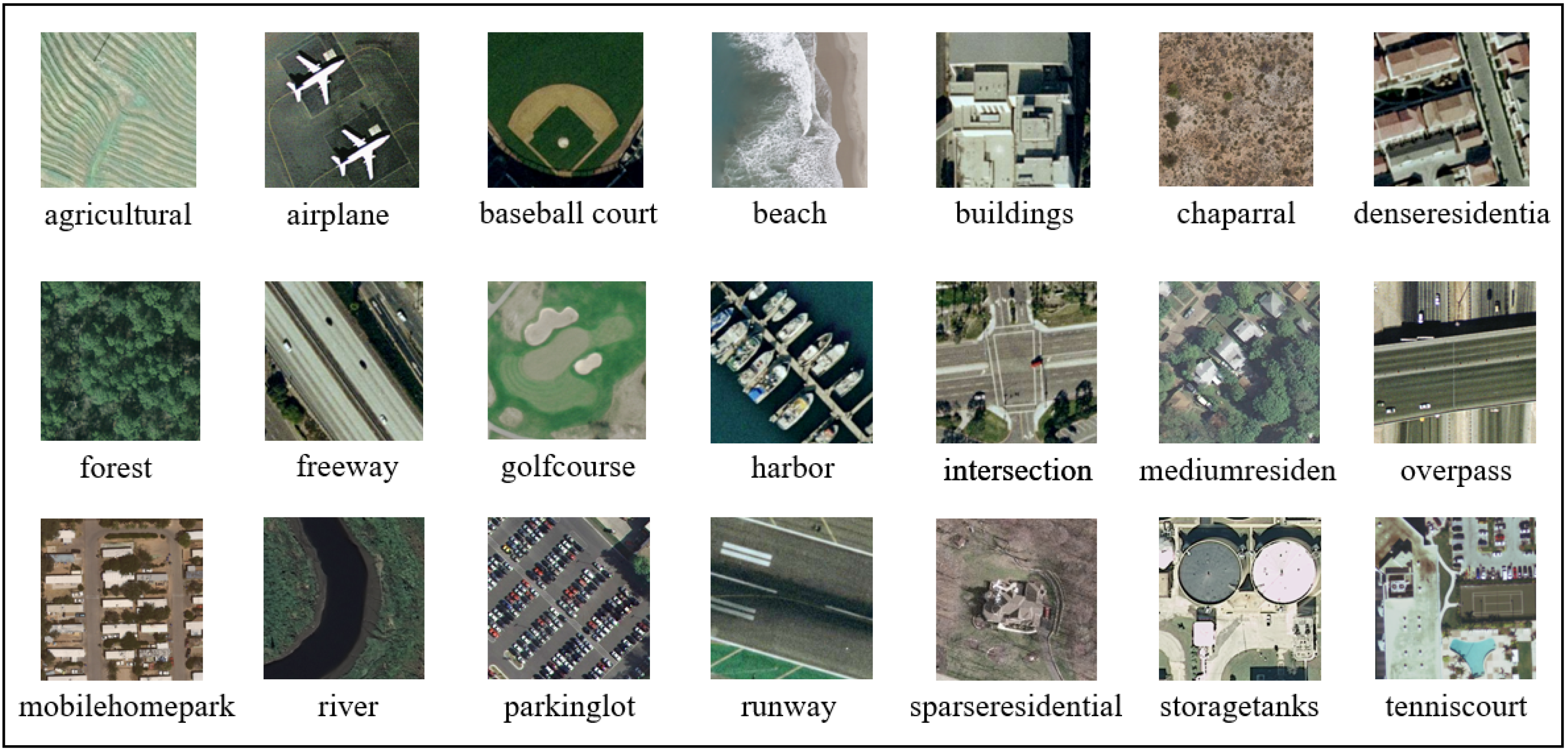
The UC Merced dataset contains 2100 images, which are divided into 10: 5: 6 for experiments; the spatial resolution of each image is 0.3 m with 256 × 256 pixels. As shown in Figure 4. Many RS scene classification researchers have applied this data set to experiments since it appeared. This data set has too much noise, so it is more classification challenging. NWPU-RESISC45 has 45 image categories, which is the most in the three data sets, and its image pixels are the same as the previous data sets. Currently, this dataset has the largest number of scene categories and image totals. WHU-RS19 is a dataset that contains 19 categories with a total of 1005 images, of which pixels are the largest in the three datasets.

The RS images are divided into three parts. Two of these are used for training and validation of the model, while another dataset evaluates the model through cross validation. For the training task, five scene categories were randomly selected from the dataset $D_{train}$ to simulate the few-shot task. Extract one and five samples from each category to form a meta-task. For each test task, five scene categories were also randomly selected in the dataset $D_{test}$, with one and five labeled samples for each scene category.

2.6. Experiment Setups

For traditional deep learning, an iteration represents the entire data set propagating forward once through a neural network. For the few-shot learning in this experiment, although one or several label samples are randomly sampled in each task, all samples are likely to be sampled when the number of tasks is large enough. 8000 training tasks were set in the experiment, the initial value of the learning rate was 0.005, and the initial parameters of the optimizer were set to 0.5. In addition, the generalization of all models is evaluated by cross-entropy loss. All experiments were set to five scene categories, with one sample and five samples selected for each scene category. Theoretically, the more samples of the scene, the higher the accuracy of the experiment. In order to avoid the model’s preference for specific data, all experiments were randomly sampled from $D_{test}$ for 15 tests. For the test results, 600 few-shot tasks were sampled to test the model, and the test results were averaged to obtain the final result.

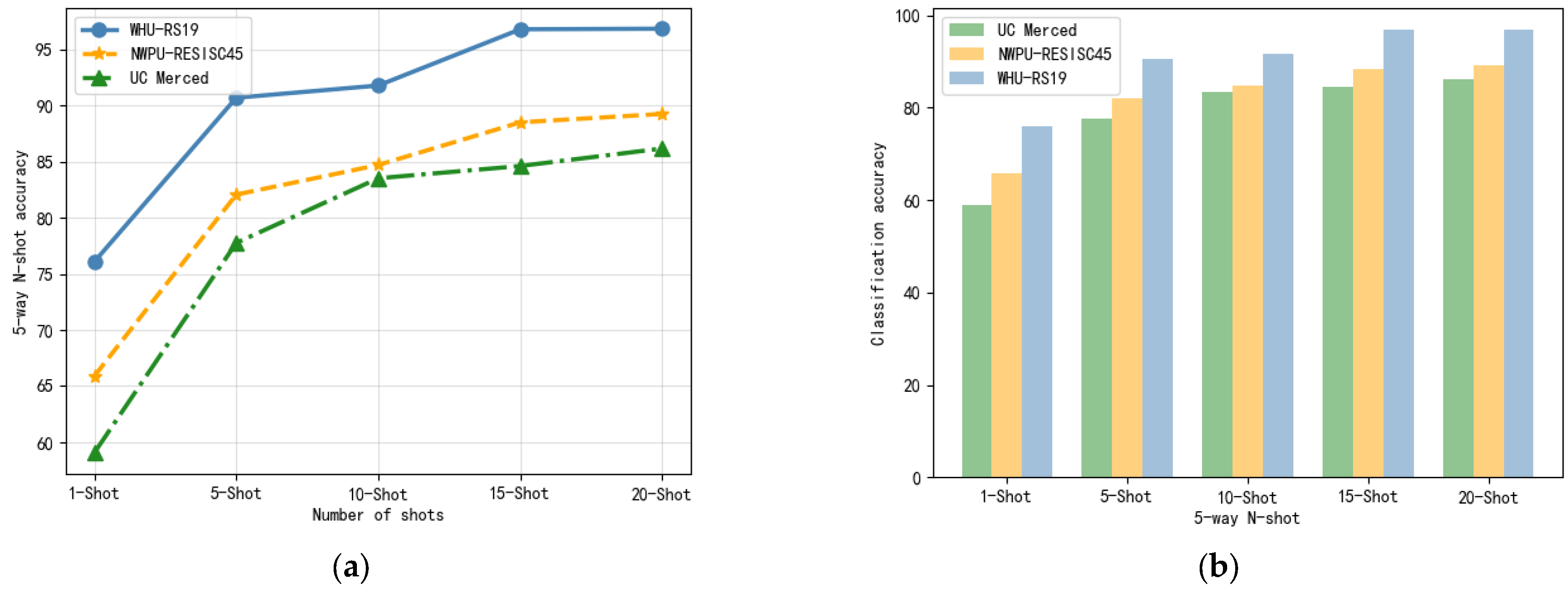
The accuracy assessment metrics of our experiment is usually N-way K-shot. N categories are selected, and K samples are selected for each category. Generally, $N\in \left\{5,10,15,20\right\}, K\in \left\{1,5\right\}$. In the model training phase, the training model is constructed and trained on the selected $N\times K$ samples. In the test phase, K samples from N categories are selected to perform the N-way K-shot classification task. According to the prediction results, the prediction category is determined, and the accuracy rate of the prediction category consistent with the actual category is the accuracy assessment metrics.

3. Results

3.1. Experiment on UC Merced Dataset

In the few-sample RS scenario, the proposed model (MLLD) performs well on the relatively complex public dataset at UC Merced.

Table 2. Classification accuracy on the UC Merced dataset.

Method	5-Way 1-Shot	5-Way 5-Shot
MAML [33]	43.65 ± 0.68	58.43 ± 0.64
MatchingNet [34]	46.16 ± 0.71	66.73 ± 0.56
Relation Network [35]	48.89 ± 0.73	64.10 ± 0.54
Meta-SGD [40]	50.52 ± 2.61	60.82 ± 2.00
Prototypical Network [6]	52.62 ± 0.70	65.93 ± 0.57
TPN [41]	53.36 ± 0.77	68.23 ± 0.52
DLA-MatchNet [23]	53.76 ± 0.60	63.01 ± 0.51
RS-MetaNet [24]	57.23 ± 0.56	76.08 ± 0.28
MLLD (ours)	59.05 ± 0.75	77.76 ± 0.52

shows the final comparison results, where the classification result is obtained by testing ten rounds. The test results are the average of 600 few-shot tasks on the new set. The other eight representative methods were compared under the 5-way 1-shot and 5-way 5-shot. Eight scene classification methods for few-shot RS images: MAML, MatchingNet, Relation Network, Meta-SGD, Prototypical Network, TPN, DLA-MatchNet, RS-MetaNet. Our model and these eight networks are based on different ways of meta-learning for effective model training, so they have better comparative value. The results in the table clearly show that our MLLD performs best compared to the other eight methods. Compared with RS-MetaNet, which applies the meta-method for training and improves generalization ability through balance loss, our model (MLLD) shows superior performance. In addition, compared with the DLA-MatchNet of the feature learning module with attention mechanisms, our model (MLLD) can also improve accuracy. Moreover, our MLLD yields 1.82% and 5.29% improvements compared with RS-MetaNet and DLA-MatchNet in the 5-way 1-shot case, respectively. In addition, our MLLD yields 1.68% and 14.75% improvements in the 5-way 5-shot case, respectively.

3.2. Experiment on WHU-RS19 Dataset

In order to illustrate the credibility of the model (MLLD) and to achieve better results for different datasets, this paper also conducted experiments on the WHU-RS19 dataset. The comparison results of the experiment are shown in

Table 3. Classification accuracy on the WHU-RS19 dataset.

Method	5-Way 1-Shot	5-Way 5-Shot
MAML [33]	46.72 ± 0.55	79.88 ± 0.41
MatchingNet [34]	60.60 ± 0.68	82.99 ± 0.40
Relation Network [35]	60.54 ± 0.71	76.24 ± 0.34
Meta-SGD [40]	51.54 ± 2.31	61.74 ± 2.02
Prototypical Network [6]	70.88 ± 0.65	85.62 ± 0.33
TPN [41]	59.28 ± 0.72	71.20 ± 0.55
DLA-MatchNet [23]	68.27 ± 1.83	79.89 ± 0.33
RS-MetaNet [24]	-	-
MLLD (ours)	76.07 ± 0.65	90.69 ± 0.27

.

After 10 rounds of testing on 600 tasks randomly sampled from the new set, the final accuracy is obtained by averaging the test results. Table 3 shows that each of the five categories was tested with one sample and five samples, and the experimental accuracy of the model proposed in this paper can reach 76.07% and 90.69%, surpassing the prototypical network with 5.19% and 5.07% improvements, respectively. It indicates that an embedded learning module with Manifold Mixup can learn robust and accurate feature representation. In addition, local descriptors can be accurately classified by measuring them.

3.3. Experiment on NWPU-RESISC45 Dataset

The images in the NWPU-RESISC45 dataset are the most in the three datasets and are assigned a ratio of 25:10:10. In the few-shot RS image scenario, the test results of the model are shown in

Table 4. Classification accuracy on the NWPU-RESISC45 dataset.

Method	5-Way 1-Shot	5-Way 5-Shot
MAML [33]	37.36 ± 0.69	45.94 ± 0.68
MatchingNet [34]	54.46 ± 0.77	67.87 ± 0.59
Relation Network [35]	58.61 ± 0.83	78.63 ± 0.52
Meta-SGD [40]	60.63 ± 0.90	75.75 ± 0.65
Prototypical Network [6]	50.82 ± 0.84	74.39 ± 0.59
TPN [41]	66.51 ± 0.87	78.50 ± 0.56
DLA-MatchNet [23]	68.80 ± 0.70	81.63 ± 0.46
RS-MetaNet [24]	52.78 ± 0.09	71.49 ± 0.81
MLLD (ours)	65.88 ± 0.83	82.06 ± 0.53

.

According to Table 4, the accuracy of the classification model can reach 65.88% and 82.06% in one sample of five categories and five samples of five categories. Compared with the DLA-MatchNet, it is improved on 5-way 5-shot, but the accuracy is 3% lower on 5-way 1-shot. The reason for this result may be that the NWPU-RESISC45 data set is more complex, the image is blurred, and the noise is more. The subsequent research can improve image quality and further enhance experimental results by denoising data sets. In addition, our experiments are better than the other models.

3.4. Ablation Studies

Figure 5 shows the loss visualization of different models on the WHU-RS19 dataset on a 5-Way 1-Shot. The information in the figure shows that after 125 iterations, the model loss of this experiment is almost 0, and there is no longer a jump in the later period. The benchmark model’s early convergence rate is very slow and difficult to achieve convergence. In this paper, the feature extractor is replaced by ResNet256 for comparison. From the information in Figure 5, it can be concluded that the speed of extracting features with ResNet256 is faster in the early stages, but after 125 iterations, there will still be a jump. It shows that MLLD can achieve more accurate and stable results when classifying different few-shot tasks. Figure 6 clearly illustrates the comparison results of our model and the baselines for training loss (a) and validation accuracy (b). The number of iterations for the training loss is 80,000. The model loss approaches zero as the number of iterations increases, and our model training loss decreases faster. The number of iterations for validation accuracy is 8000, and Figure 6b shows that our validation accuracy is higher than the baseline.

Figure 7 shows the results of the ablation experiment on three datasets. The model (MLLD) in this paper has a greater improvement, that is, this model shows a significant effect on few-shot tasks, especially when one sample per category is more sensitive. The effect is best in the WHU-RS19 dataset, indicating that the model is more accurate for feature extraction from training samples in this dataset.

Figure 8 shows the classification accuracy of the datasets used in this paper in five categories, with 1, 5, 10, 15, and 20 samples in each category. The information in the figure indicates that the classification result is proportional to the number of samples, and along with the increase in samples, the classification correct probability is also constantly improving. However, the classification accuracy increases faster on 1-shot to 5-shot, and the classification accuracy increases more slowly on 10-shot to 20-shot, indicating that the model is more effective for few-shot. The final results on the data sets WHU-RS19, NWPU-RESISC45, and UC Merced indicate that the model in this paper is more sensitive to WHU-RS19, while the UC Merced data set is more complex, more noisy, and more difficult to distinguish.

4. Discussion

The application requirements of remote sensing image scenes in urban supervision, resource exploration, and natural disaster detection are gradually increasing. Therefore, remote sensing scene classification is an urgent problem that needs to be solved. However, due to the characteristics of background confusion and image noise in RS images, as well as the boundary blurring of neural networks, the classification accuracy will be reduced. Therefore, this paper proposes a classification method based on metric learning and local descriptors (MLLD), which structures an embedded learning module and a metric module. The embedded learning module learns model parameters through meta-training on multiple few-shot tasks, then extracts features through a four-layer convolutional network and fuses feature vectors and labels. The visual representation of the sample is concentrated in a low-dimensional subspace to produce more discriminative features. The feature vector is divided into local descriptors, and then the similarity between the image and the category is calculated by the measurement module according to the local feature invariance.

The summary of this paper is summarized as follows:

By studying the data augmentation strategy, a novel embedded learning module with the data-dependent regularization operation is added. This module adds Manifold Mixup to smooth the decision boundary and learn accurate feature representation in few-shot RS scene classification.

According to local invariant features, we replace the metric based on image-level features with an image-to-class metric based on local descriptors. The measurement based on local features can effectively avoid the error caused by image-level feature representation and prevent the loss of some discriminative information that leads to inaccurate measurement.

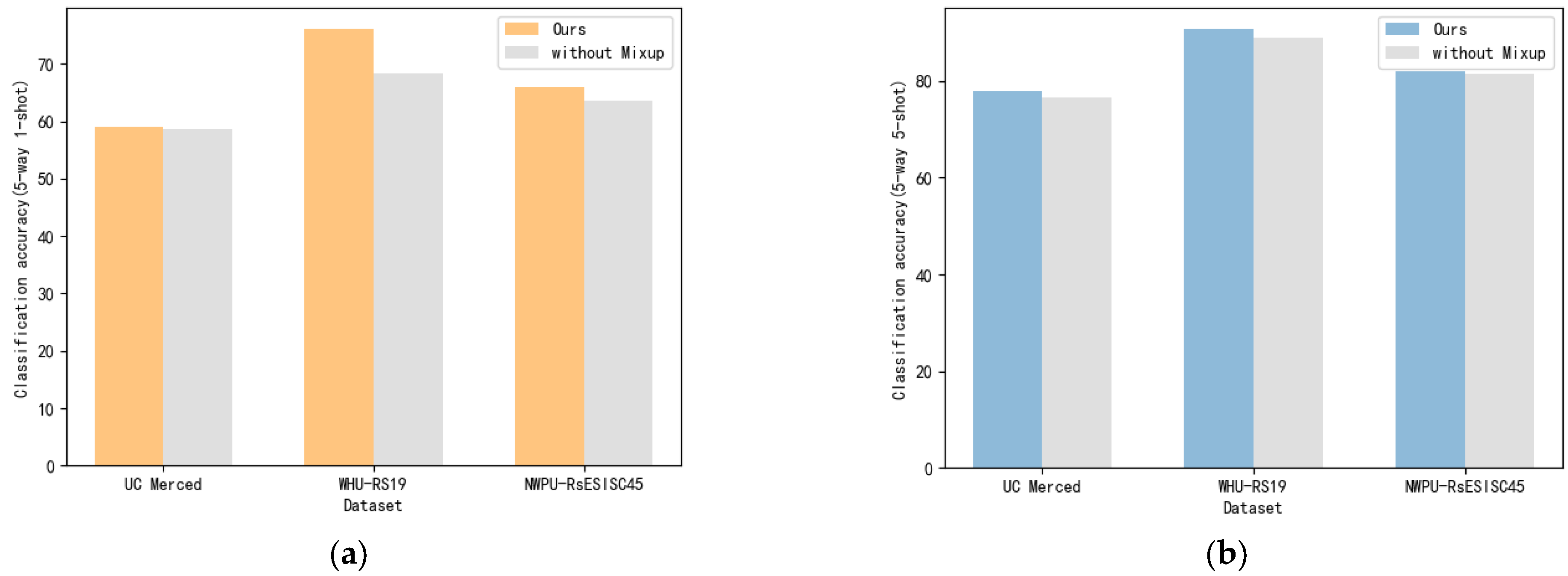
Experiments were conducted on three remote sensing data sets, namely UC Merced, WHU-RS19, and NWPU-RESISC45. Experimental results show that our model (MLLD) has a significant effect on few-shot RS image classification, which can improve the shortcomings of previous models and further enhance the classification accuracy. The classification result of the three datasets on a 5-way 1-shot can reach 59.05%, 65.88%, and 76.07%, respectively, and on a 5-way 5-shot, it can reach 77.76%, 82.06%, and 90.69%, respectively. Experiments show that the embedded learning module based on Manifold Mixup and the measurement module based on local descriptors are proven to effectively improve the classification accuracy of a few-shot RS image.