
Estimation of Ground-Level PM2.5 Concentration at Night in Beijing-Tianjin-Hebei Region with NPP/VIIRS Day/Night Band


Abstract
1. Introduction
2. Materials and Methods
2.1. Data Collection
- (1)
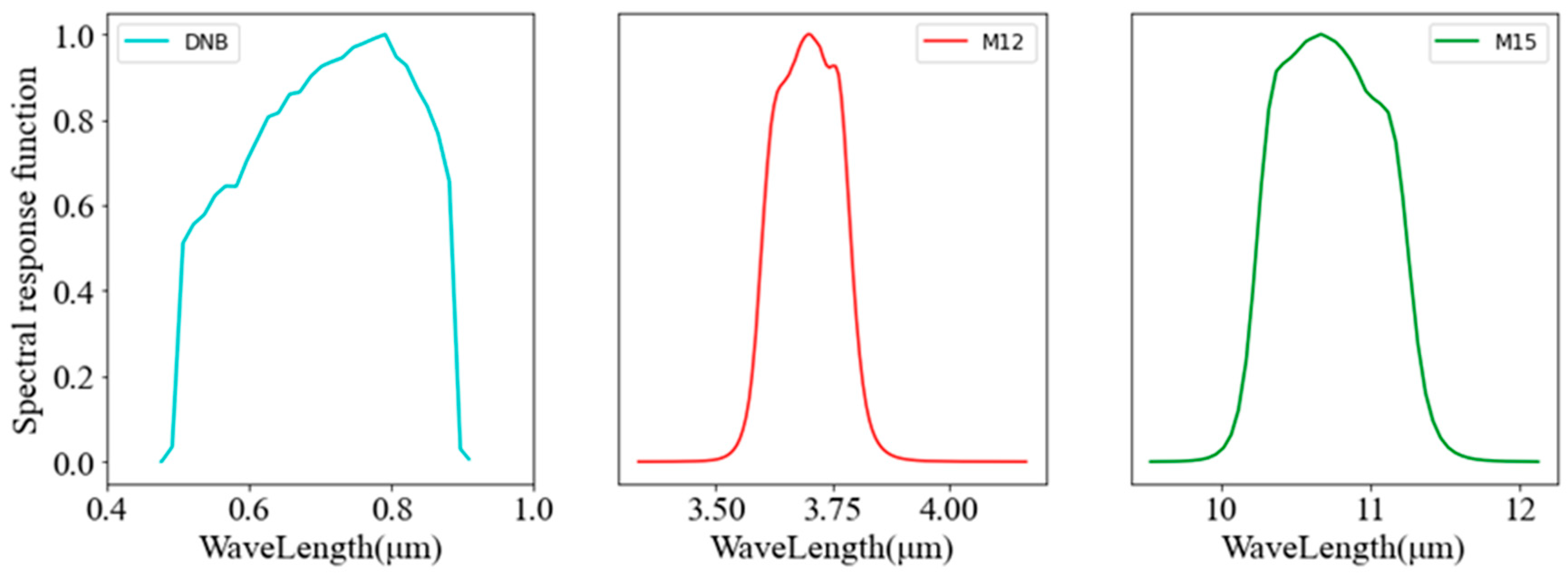
- Satellite data
- (2)
- Meteorological data
- (3)
- Ground PM2.5 data
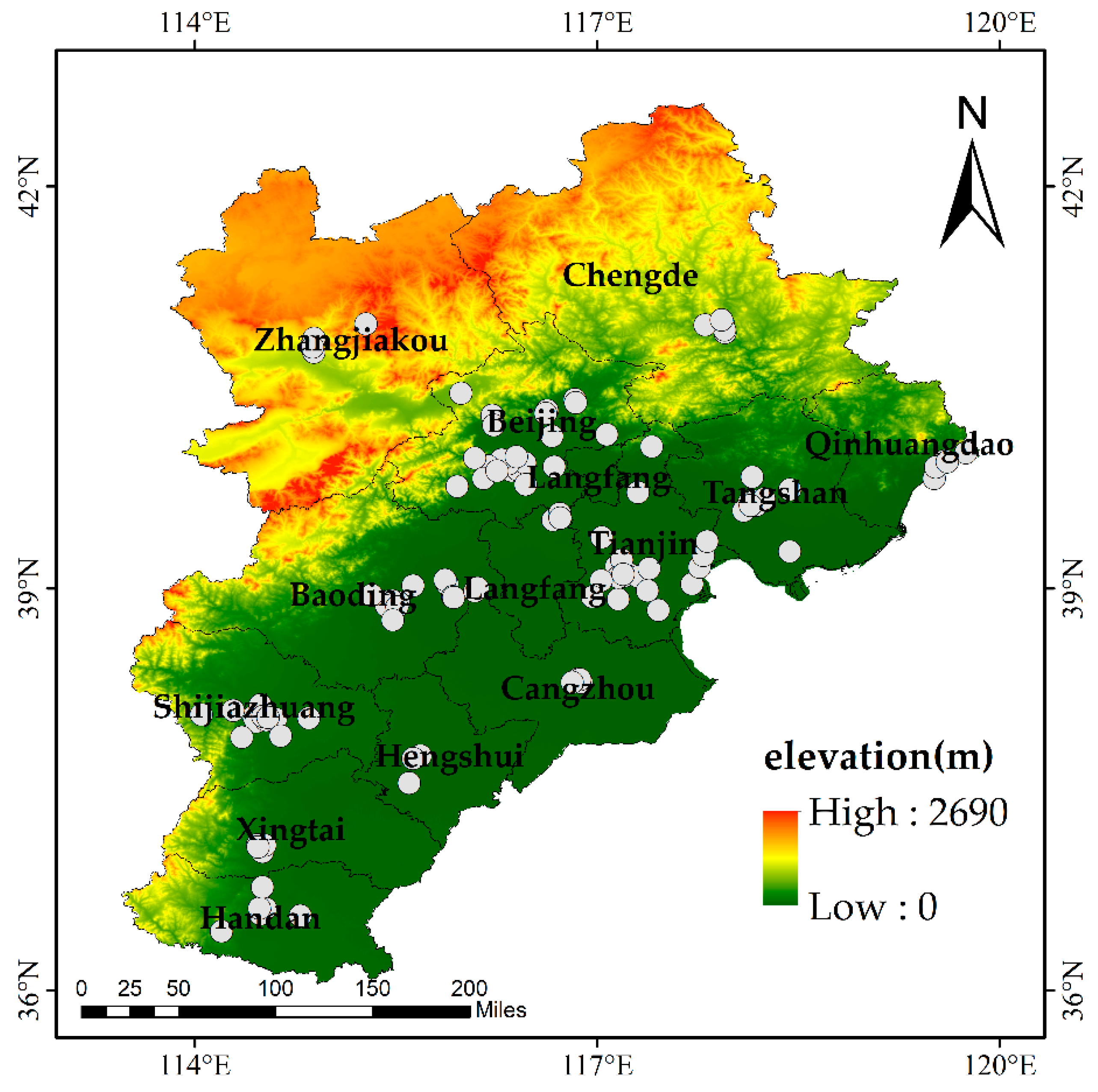
2.2. Research Region
2.3. Methods
- (1)
- Data collection and processing: The study used ground monitoring of PM2.5 concentration, satellite, and meteorological (SP, PBLH, AT, RH, and WS) data. These data were preprocessed and spatiotemporally matched. Preprocessing involved geometric correction, cloud removal, cropping of satellite data, resampling and cutting of meteorological data, and removal of missing data (NAN) from the ground PM2.5 data.
- (2)
- Model building: The processed data set was trained with the random forest model, and the optimal parameters of the model were determined with the grid search. The grid search used the exhaustive method to search for the optimal parameters. The essence was to train the combination of all parameters and calculate the mean square error (MSE) of the corresponding model. Finally, the parameter combination with the minimum MSE was obtained, which was the optimal parameter combination of the model [35].
- (3)
- Model accuracy evaluation: A 10-fold, cross-validation was performed. The model accuracy was evaluated with the RMSE, determination coefficient (R2), and mean absolute error (MAE). The final NightPMES model was selected if it had sufficient precision; otherwise, the parameters were adjusted.
- (4)
- The estimation of the nighttime PM2.5 concentration in the BTH region was performed by entering data (locations without surface PM2.5 observations) into the NightPMES model.
2.3.1. NightPMES Model
2.3.2. Seasonal Model
3. Results
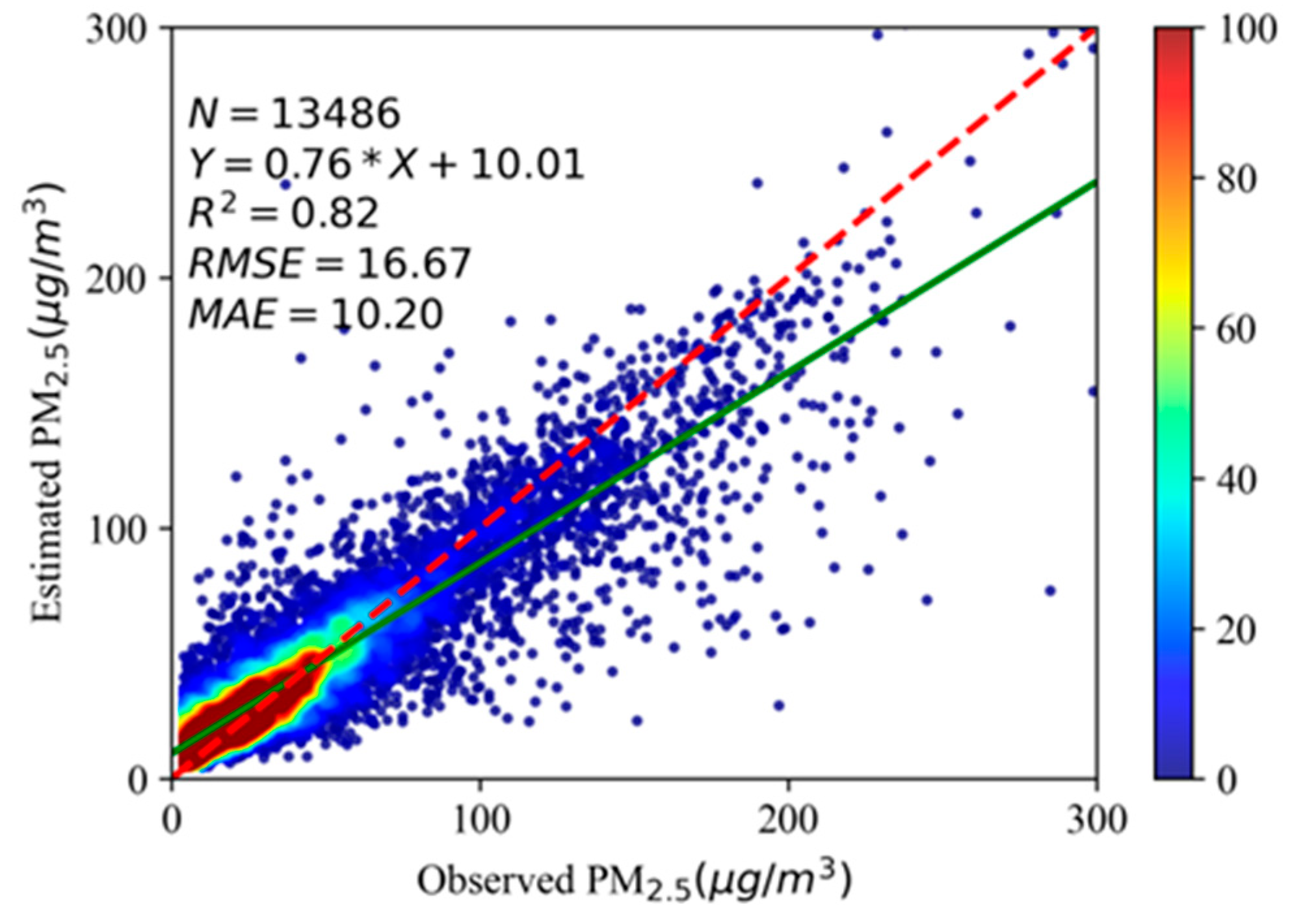
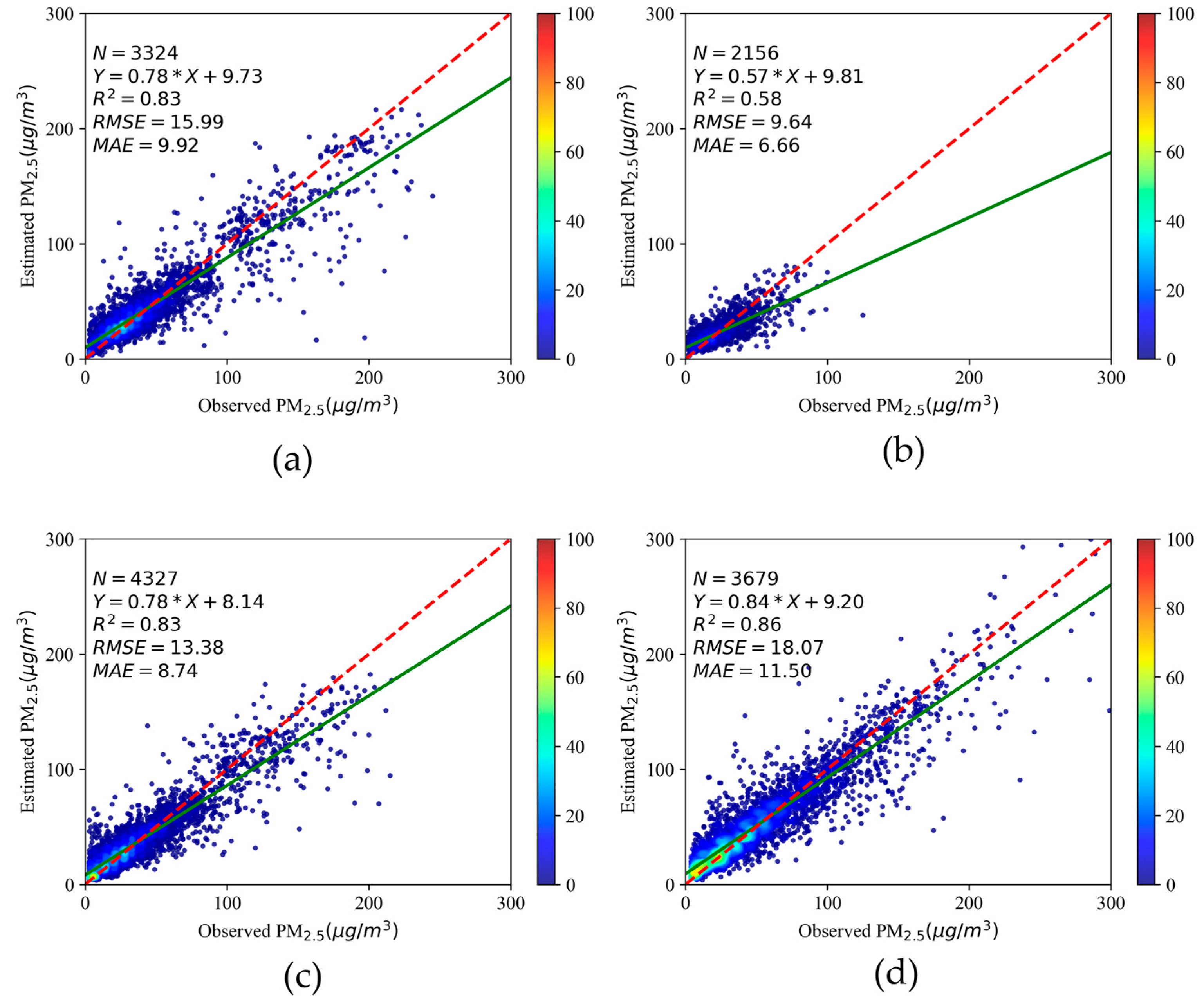
3.1. Comparison of Different Models
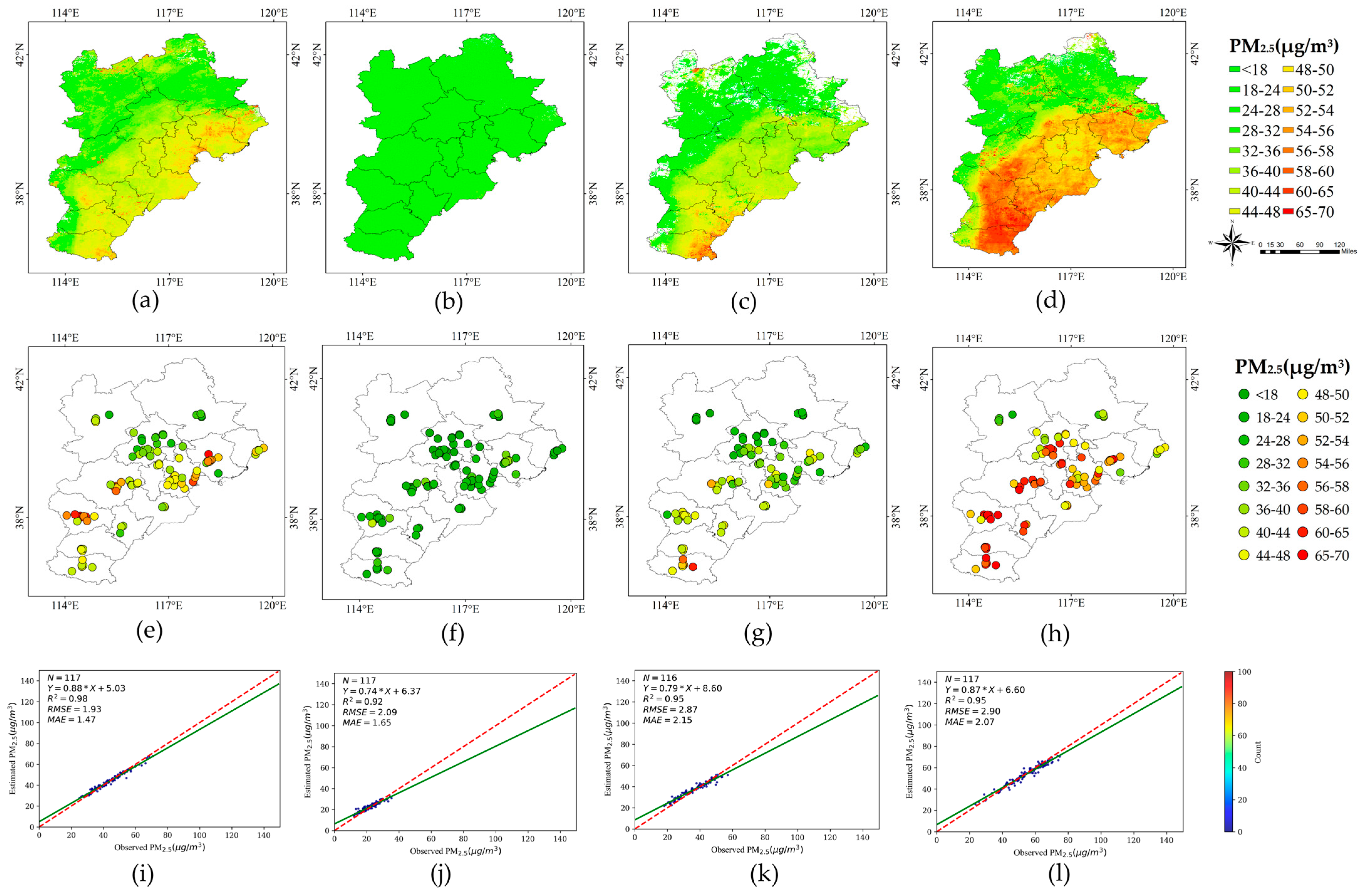
3.2. Temporal and Spatial Distribution of Nighttime PM2.5 Concentration
3.3. Effect of Moon Phase Angle on Nighttime PM2.5 Concentration
3.4. Effect of Seasonal Characteristics on Nighttime PM2.5 Concentration
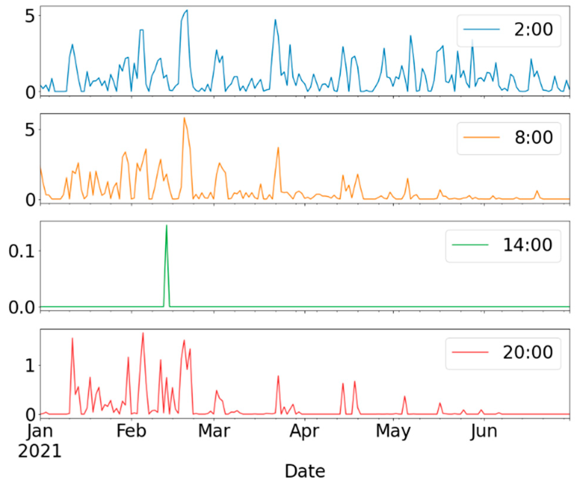
3.5. Analysis of the Diurnal Variation of PM2.5 Concentration
4. Discussion
5. Conclusions
Author Contributions
Funding
Conflicts of Interest
References
- Zhang, D.; Du, L.; Wang, W.; Zhu, Q.; Bi, J.; Scovronick, N.; Naidoo, M.; Garland, R.M.; Liu, Y. A Machine Learning Model to Estimate Ambient PM2.5 Concentrations in Industrialized Highveld Region of South Africa. Remote Sens. Environ. 2021, 266, 112713. [Google Scholar] [CrossRef]
- World Health Organization. WHO Global Air Quality Guidelines: Particulate Matter (PM2.5 and PM10), Ozone, Nitrogen Dioxide, Sulfur Dioxide and Carbon Monoxide; World Health Organization: Geneva, Switzerland, 2021. [Google Scholar]
- Xie, R.; Sabel, C.E.; Lu, X.; Zhu, W.; Kan, H.; Nielsen, C.P.; Wang, H. Long-Term Trend and Spatial Pattern of PM2.5 Induced Premature Mortality in China. Environ. Int. 2016, 97, 180–186. [Google Scholar] [CrossRef] [PubMed]
- Vodonos, A.; Awad, Y.A.; Schwartz, J. The Concentration-Response between Long-Term PM 2.5 Exposure and Mortality; A Meta-Regression Approach. Environ. Res. 2018, 166, 677–689. [Google Scholar] [CrossRef] [PubMed]
- Mousavi, S.E.; Amini, H.; Heydarpour, P.; Amini Chermahini, F.; Godderis, L. Air Pollution, Environmental Chemicals, and Smoking May Trigger Vitamin D Deficiency: Evidence and Potential Mechanisms. Environ. Int. 2019, 122, 67–90. [Google Scholar] [CrossRef] [PubMed]
- Amini, H.; Trang Nhung, N.T.; Schindler, C.; Yunesian, M.; Hosseini, V.; Shamsipour, M.; Hassanvand, M.S.; Mohammadi, Y.; Farzadfar, F.; Vicedo-Cabrera, A.M.; et al. Short-Term Associations between Daily Mortality and Ambient Particulate Matter, Nitrogen Dioxide, and the Air Quality Index in a Middle Eastern Megacity. Environ. Pollut. 2019, 254, 113121. [Google Scholar] [CrossRef]
- Coleman, C.J.; Yeager, R.A.; Pond, Z.A.; Riggs, D.W.; Bhatnagar, A.; Arden Pope, C. Mortality Risk Associated with Greenness, Air Pollution, and Physical Activity in a Representative U.S. Cohort. Sci. Total Environ. 2022, 824, 153848. [Google Scholar] [CrossRef]
- Zhang, L.; Wilson, J.P.; MacDonald, B.; Zhang, W.; Yu, T. The Changing PM2.5 Dynamics of Global Megacities Based on Long-Term Remotely Sensed Observations. Environ. Int. 2020, 142, 105862. [Google Scholar] [CrossRef]
- Weichenthal, S.; Pinault, L.; Christidis, T.; Burnett, R.T.; Brook, J.R.; Chu, Y.; Crouse, D.L.; Erickson, A.C.; Hystad, P.; Li, C.; et al. How Low Can You Go? Air Pollution Affects Mortality at Very Low Levels. Sci. Adv. 2022, 8, eabo3381. [Google Scholar] [CrossRef]
- Peng, J.; Han, H.; Yi, Y.; Huang, H.; Xie, L. Machine Learning and Deep Learning Modeling and Simulation for Predicting PM2.5 Concentrations. Chemosphere 2022, 308, 136353. [Google Scholar] [CrossRef] [PubMed]
- Wei, J.; Li, Z.; Lyapustin, A.; Sun, L.; Peng, Y.; Xue, W.; Su, T.; Cribb, M. Reconstructing 1-Km-Resolution High-Quality PM2.5 Data Records from 2000 to 2018 in China: Spatiotemporal Variations and Policy Implications. Remote Sens. Environ. 2021, 252, 112136. [Google Scholar] [CrossRef]
- Zhang, L.; Wilson, J.P.; Zhao, N.; Zhang, W.; Wu, Y. The Dynamics of Cardiovascular and Respiratory Deaths Attributed to Long-Term PM2.5 Exposures in Global Megacities. Sci. Total Environ. 2022, 842, 156951. [Google Scholar] [CrossRef] [PubMed]
- Zhang, W.; Zheng, F.; Zhang, W.; Yang, X. Estimating Ground-Level Hourly PM2.5 Concentrations Over North China Plain with Deep Neural Networks. J. Indian Soc. Remote Sens. 2021, 49, 1839–1852. [Google Scholar] [CrossRef]
- Li, R.; Liu, X.; Li, X. Estimation of the PM2.5 Pollution Levels in Beijing Based on Nighttime Light Data from the Defense Meteorological Satellite Program-Operational Linescan System. Atmosphere 2015, 6, 607–622. [Google Scholar] [CrossRef]
- Chen, G.; Li, S.; Knibbs, L.D.; Hamm, N.A.S.; Cao, W.; Li, T.; Guo, J.; Ren, H.; Abramson, M.J.; Guo, Y. A Machine Learning Method to Estimate PM2.5 Concentrations across China with Remote Sensing, Meteorological and Land Use Information. Sci. Total Environ. 2018, 636, 52–60. [Google Scholar] [CrossRef] [PubMed]
- Ma, Z.; Dey, S.; Christopher, S.; Liu, R.; Bi, J.; Balyan, P.; Liu, Y. A Review of Statistical Methods Used for Developing Large-Scale and Long-Term PM2.5 Models from Satellite Data. Remote Sens. Environ. 2022, 269, 112827. [Google Scholar] [CrossRef]
- Hidy, G.M.; Brook, J.R.; Chow, J.C.; Green, M.; Husar, R.B.; Lee, C.; Scheffe, R.D.; Swanson, A.; Watson, J.G. Remote Sensing of Particulate Pollution from Space: Have We Reached the Promised Land? J. Air Waste Manag. Assoc. 2009, 59, 1130–1139. [Google Scholar] [CrossRef] [PubMed]
- Li, S.; Joseph, E.; Min, Q. Remote Sensing of Ground-Level PM2.5 Combining AOD and Backscattering Profile. Remote Sens. Environ. 2016, 183, 120–128. [Google Scholar] [CrossRef]
- Yazdi, M.D.; Kuang, Z.; Dimakopoulou, K.; Barratt, B.; Suel, E.; Amini, H.; Lyapustin, A.; Katsouyanni, K.; Schwartz, J. Predicting Fine Particulate Matter (PM2.5) in the Greater London Area: An Ensemble Approach Using Machine Learning Methods. Remote Sens. 2020, 12, 914. [Google Scholar] [CrossRef]
- Feng, Y.; Fan, S.; Xia, K.; Wang, L. Estimation of Regional Ground-Level PM2.5 Concentrations Directly from Satellite Top-of-Atmosphere Reflectance Using A Hybrid Learning Model. Remote Sens. 2022, 14, 2714. [Google Scholar] [CrossRef]
- Miller, S.D.; Turner, R.E. A Dynamic Lunar Spectral Irradiance Data Set for NPOESS/VIIRS Day/Night Band Nighttime Environmental Applications. IEEE Trans. Geosci. Remote Sens. 2009, 47, 2316–2329. [Google Scholar] [CrossRef]
- Cao, C.; De Luccia, F.J.; Xiong, X.; Wolfe, R.; Weng, F. Early On-Orbit Performance of the Visible Infrared Imaging Radiometer Suite Onboard the Suomi National Polar-Orbiting Partnership (S-NPP) Satellite. IEEE Trans. Geosci. Remote Sens. 2014, 52, 1142–1156. [Google Scholar] [CrossRef]
- Johnson, R.S.; Zhang, J.; Hyer, E.J.; Miller, S.D.; Reid, J.S. Preliminary Investigations toward Nighttime Aerosol Optical Depth Retrievals from the VIIRS Day/Night Band. Atmos. Meas. Tech. 2013, 6, 1245–1255. [Google Scholar] [CrossRef]
- McHardy, T.M.; Zhang, J.; Reid, J.S.; Miller, S.D.; Hyer, E.J.; Kuehn, R.E. An Improved Method for Retrieving Nighttime Aerosol Optical Thickness from the VIIRS Day/Night Band. Atmos. Meas. Tech. 2015, 8, 4773–4783. [Google Scholar] [CrossRef]
- Zhang, J.; Jaker, S.L.; Reid, J.S.; Miller, S.D.; Solbrig, J.; Toth, T.D. Characterization and Application of Artificial Light Sources for Nighttime Aerosol Optical Depth Retrievals Using the Visible Infrared Imager Radiometer Suite Day/Night Band. Atmos. Meas. Tech. 2019, 12, 3209–3222. [Google Scholar] [CrossRef]
- Wang, J.; Aegerter, C.; Xu, X.; Szykman, J.J. Potential Application of VIIRS Day/Night Band for Monitoring Nighttime Surface PM2.5 Air Quality from Space. Atmos. Environ. 2016, 124, 55–63. [Google Scholar] [CrossRef]
- Zhao, X.; Shi, H.; Yu, H.; Yang, P. Inversion of Nighttime PM2.5 Mass Concentration in Beijing Based on the VIIRS Day-Night Band. Atmosphere 2016, 7, 136. [Google Scholar] [CrossRef]
- Fu, D.; Xia, X.; Duan, M.; Zhang, X.; Li, X.; Wang, J.; Liu, J. Mapping Nighttime PM2.5 from VIIRS DNB Using a Linear Mixed-Effect Model. Atmos. Environ. 2018, 178, 214–222. [Google Scholar] [CrossRef]
- Erkin, N.; Simayi, M.; Ablat, X.; Yahefu, P.; Maimaiti, B. Predicting Spatiotemporal Variations of PM2.5 Concentrations during Spring Festival for County-Level Cities in China Using VIIRS-DNB Data. Atmos. Environ. 2022, 294, 119484. [Google Scholar] [CrossRef]
- Wu, J.; Yao, F.; Li, W.; Si, M. VIIRS-Based Remote Sensing Estimation of Ground-Level PM2.5 Concentrations in Beijing–Tianjin–Hebei: A Spatiotemporal Statistical Model. Remote Sens. Environ. 2016, 184, 316–328. [Google Scholar] [CrossRef]
- Hu, S.; Ma, S.; Yan, W.; Jiang, J.; Huang, Y. A New Multichannel Threshold Algorithm Based on Radiative Transfer Characteristics for Detecting Fog/Low Stratus Using Night-Time NPP/VIIRS Data. Int. J. Remote Sens. 2017, 38, 5919–5933. [Google Scholar] [CrossRef]
- Liao, L.B.; Weiss, S.; Mills, S.; Hauss, B. Suomi NPP VIIRS Day-Night Band on-Orbit Performance. J. Geophys. Res. Atmos. 2013, 118, 12705–12718. [Google Scholar] [CrossRef]
- Xia, L.; Mao, K.; Sun, Z.; Ma, Y. Introduction of Suomi NPP VIIRS and Its Application on Cloud Detection. Adv. Geosci 2013, 3, 6. [Google Scholar] [CrossRef]
- Ali, M.A.; Bilal, M.; Wang, Y.; Nichol, J.E.; Mhawish, A.; Qiu, Z.; de Leeuw, G.; Zhang, Y.; Zhan, Y.; Liao, K.; et al. Accuracy Assessment of CAMS and MERRA-2 Reanalysis PM2.5 and PM10 Concentrations over China. Atmos. Environ. 2022, 288, 119297. [Google Scholar] [CrossRef]
- Abbaszadeh, M.; Soltani-Mohammadi, S.; Ahmed, A.N. Optimization of Support Vector Machine Parameters in Modeling of Iju Deposit Mineralization and Alteration Zones Using Particle Swarm Optimization Algorithm and Grid Search Method. Comput. Geosci. 2022, 165, 105140. [Google Scholar] [CrossRef]
- Guo, B.; Zhang, D.; Pei, L.; Su, Y.; Wang, X.; Bian, Y.; Zhang, D.; Yao, W.; Zhou, Z.; Guo, L. Estimating PM2.5 Concentrations via Random Forest Method Using Satellite, Auxiliary, and Ground-Level Station Dataset at Multiple Temporal Scales across China in 2017. Sci. Total Environ. 2021, 778, 146288. [Google Scholar] [CrossRef]
- Bera, B.; Bhattacharjee, S.; Sengupta, N.; Saha, S. PM2.5 Concentration Prediction during COVID-19 Lockdown over Kolkata Metropolitan City, India Using MLR and ANN Models. Environ. Challenges 2021, 4, 100155. [Google Scholar] [CrossRef]
- She, L.; Zhang, H.K.; Li, Z.; de Leeuw, G.; Huang, B. Himawari-8 Aerosol Optical Depth (Aod) Retrieval Using a Deep Neural Network Trained Using Aeronet Observations. Remote Sens. 2020, 12, 4125. [Google Scholar] [CrossRef]
- Zhao, X.; Shi, H.; Yang, P.; Zhang, L.; Fang, X.; Liang, K. Inversion Algorithm of PM2.5 Air Quality Based on Nighttime Light Data from NPP-VIIRS. J. Remote Sens. 2017, 21, 291–299. [Google Scholar] [CrossRef]
- Li, K.; Liu, C.; Jiao, P. Estimating of Nighttime PM2.5 Concentrations in Shanghai Based on NPP/VIIRS Day_Night Band Data. Acta Sci. Circumstantiae 2019, 39, 1913–1922. [Google Scholar] [CrossRef]
- Chen, H.; Xu, Y.; Mo, Y.; Zhang, Y.; Yang, Z. Estimating Nighttime PM2.5 Concentrations in Huai’an Based on NPP/VIIRS Nighttime Light Data. Acta Sci. Circumstantiae 2022, 42, 342–351. [Google Scholar] [CrossRef]
- Sager, L. Estimating the Effect of Air Pollution on Road Safety Using Atmospheric Temperature Inversions. J. Environ. Econ. Manag. 2019, 98, 102250. [Google Scholar] [CrossRef]
- Wei, J.; Li, Z. ChinaHighPM2.5: Big Data Seamless 1 km Ground-Level PM2.5 Dataset for China; Version 4; Data Set; Zenodo: Geneva, Switzerland, 2019. [Google Scholar] [CrossRef]
- Wei, J.; Li, Z.; Cribb, M.; Huang, W.; Xue, W.; Sun, L.; Guo, J.; Peng, Y.; Li, J.; Lyapustin, A.; et al. Improved 1 Km Resolution PM2.5 Estimates across China Using Enhanced Space-Time Extremely Randomized Trees. Atmos. Chem. Phys. 2020, 20, 3273–3289. [Google Scholar] [CrossRef]
- Kieffer, H.H.; Anderson, J.M. Use of the Moon for Spacecraft Calibration over 350 to 2500 Nm. In Sensors, Systems and Next-Generation Satellites II; SPIE: Bellingham, WA, USA, 1998; Volume 3498, pp. 325–336. [Google Scholar] [CrossRef]
- Kieffer, H.H.; Stone, T.C. The Spectral Irradiance of the Moon. Astron. J. 2005, 129, 2887–2901. [Google Scholar] [CrossRef]


| Category | Variable | Units | Spatial Resolution | Temporal Resolution |
|---|---|---|---|---|
| Satellite data | DNB radiance | W/(sr·m2) | 750 m | Daily |
| moon phase angle | degree | - | Daily | |
| Meteorological data | PBLH 1 | m | 0.5° × 0.625° | Hourly |
| SP 2 | Pa | 0.5° × 0.625° | Hourly | |
| AT 3 | K | 0.5° × 0.625° | Hourly | |
| RH 4 | % | 0.5° × 0.625° | Hourly | |
| WS 5 | m/s | 0.5° × 0.625° | Hourly | |
| Ground PM2.5 data | PM2.5 | µg/m3 | - | Hourly |
| Parameter | Meaning | Value |
|---|---|---|
| n_estimators | Number of trees | 240 |
| max_depth | Maximum tree depth | 46 |
| Season | Parameter | Value |
|---|---|---|
| Spring | n_estimators | 100 |
| max_depth | 20 | |
| Summer | n_estimators | 100 |
| max_depth | 20 | |
| Autumn | n_estimators | 100 |
| max_depth | 25 | |
| Winter | n_estimators | 100 |
| max_depth | 25 |
| Name | Value |
|---|---|
| Hidden layers number | 4 |
| Number of neurons | 1024, 512, 256, 128 |
| ActivationMethod | ReLU |
| Regularization | dropout |
| Number of iterations | 1500 |
| Loss function | MAE |
| Optimization functions | Adam |
| Initial learning rate | 0.001 |
| Model | R2 | RMSE (µg/m3) | MAE (µg/m3) |
|---|---|---|---|
| MLR | 0.13 | 34.44 | 23.63 |
| DNN | 0.74 | 20.18 | 12.46 |
| NightPMES | 0.82 | 16.67 | 10.20 |
| Model | Number of Sites | Sample Size | R2 | RMSE (µg/m3) | Reference |
|---|---|---|---|---|---|
| MLR | 5 | 75 | 0.45 | 4.114 | Wang et al. (2016) [26] |
| SVM | 4 | 50 | 0.90 | - | Zhao et al. (2017) [39] |
| BP | 12 | 198 | 0.83 | 14.02 | Zhao et al. (2016) [27] |
| MLR | 9 | 488 | 0.77 | 19.21 | Li et al. (2019) [40] |
| SVM | 18 | 324 | 0.77 | 32.05 | Chen et al. (2022) [41] |
| NightPMES | 121 | 13486 | 0.82 | 16.67 | This study |
Disclaimer/Publisher’s Note: The statements, opinions and data contained in all publications are solely those of the individual author(s) and contributor(s) and not of MDPI and/or the editor(s). MDPI and/or the editor(s) disclaim responsibility for any injury to people or property resulting from any ideas, methods, instructions or products referred to in the content. |
© 2023 by the authors. Licensee MDPI, Basel, Switzerland. This article is an open access article distributed under the terms and conditions of the Creative Commons Attribution (CC BY) license (https://creativecommons.org/licenses/by/4.0/).
Share and Cite
Ma, Y.; Zhang, W.; Zhang, L.; Gu, X.; Yu, T. Estimation of Ground-Level PM2.5 Concentration at Night in Beijing-Tianjin-Hebei Region with NPP/VIIRS Day/Night Band. Remote Sens. 2023, 15, 825. https://doi.org/10.3390/rs15030825
Ma Y, Zhang W, Zhang L, Gu X, Yu T. Estimation of Ground-Level PM2.5 Concentration at Night in Beijing-Tianjin-Hebei Region with NPP/VIIRS Day/Night Band. Remote Sensing. 2023; 15(3):825. https://doi.org/10.3390/rs15030825
Chicago/Turabian StyleMa, Yu, Wenhao Zhang, Lili Zhang, Xingfa Gu, and Tao Yu. 2023. "Estimation of Ground-Level PM2.5 Concentration at Night in Beijing-Tianjin-Hebei Region with NPP/VIIRS Day/Night Band" Remote Sensing 15, no. 3: 825. https://doi.org/10.3390/rs15030825
APA StyleMa, Y., Zhang, W., Zhang, L., Gu, X., & Yu, T. (2023). Estimation of Ground-Level PM2.5 Concentration at Night in Beijing-Tianjin-Hebei Region with NPP/VIIRS Day/Night Band. Remote Sensing, 15(3), 825. https://doi.org/10.3390/rs15030825