Article

Integrated Convective Characteristic Extraction Algorithm for Dual Polarization Radar: Description and Application to a Convective System

1
School of Atmospheric Physics, Nanjing University of Information Science and Technology, Nanjing 210044, China
2
Key Laboratory of Severe Weather, Chinese Academy of Meteorological Sciences, Beijing 100081, China
*
Author to whom correspondence should be addressed.
Remote Sens. 2023, 15(3), 808; https://doi.org/10.3390/rs15030808
Submission received: 5 January 2023 / Revised: 30 January 2023 / Accepted: 30 January 2023 / Published: 31 January 2023

Abstract

:
To further enhance the application of dual-polarization radar in hail nowcasting, we develop an integrated convective characteristic extraction (ICCE) algorithm based on the storm cell identification and tracking (SCIT) algorithm using dual-polarization radar data and its secondary products (hydrometeor classification data and mesocyclone data). The ICCE identifies and tracks not storm cells but convective systems, and it adds other storm characteristics, such as storm microphysics (hail- and graupel-related) and storm dynamics (mesocyclone-related), to the original storm characteristics, such as storm structure (reflectivity-related) and storm tracking (motion-related). The data of four mesocyclonic hailstorms observed by the two S-band dual-polarization radars in Guangdong Province, China, are utilized, from which we draw the following conclusions: (1) ICCE excels in identifying, characterizing, matching, and tracking convective systems; and (2) the newly added storm microphysics and dynamics characteristics can more accurately quantify the relationship between mesocyclone development, hail growth, and convective system enhancement throughout the evolution of the convective system.

Graphical Abstract

1. Introduction

Hailstorms and their accompanying hail, gales, short-term heavy rainfall, and tornadoes pose huge threats to human life and property. Weather radar plays an important role in observing hailstorms and the early warning of these severe weather events [1,2,3,4,5,6]. Storm identification and tracking algorithms, which use single-polarization radar observations to identify storms, calculate structural storm characteristics—such as centroid position, vertically integrated liquid water (VIL), maximum reflectivity, top height, area, and so on—and track and forecast the location and strength of storms, constitute a key part of severe weather warning operations [2,3]. On the one hand, these output storm structural characteristics can also serve as input to other reflectivity-based severe weather detection algorithms, such as hail detection algorithms [4,5,6]. On the other hand, the algorithms that provide the temporal trends of structural storm characteristics are also suitable for studying the physical mechanisms of storm evolution and, thus, provide an important tool for nowcasting [2,3]. However, better hail nowcasting also requires the inclusion of microphysical (e.g., hail and graupel) and dynamical (e.g., mesocyclones) characteristics of storms. Therefore, the more advanced dual-polarization radar, which can distinguish hydrometeor types such as rain, hail, graupel, and snow in each radar range bin through the hydrometeor classification (HC) algorithm [7,8], provides a key means to further improve nowcasting capabilities. However, the HC algorithms can only output products in real time and provide no way of forecasting the hydrometeor evolution of storms [7,8]. As such, based on the dual-polarization radar data and its secondary products (hydrometeor classification data and mesocyclone data), the development of a method for identifying and tracking hailstorms while also calculating the trends of their structural, microphysical, and dynamical characteristics is essential for hail nowcasting.
The original hail nowcasting approach using reflectivity data is mainly faced with the difficulties of low detection accuracy and poor forecasting precision [5,6]. These difficulties can be described in terms of the following three points: first, the parameter thresholds in hail detection methods should vary with time and location, and fixing empirical thresholds can lead to bias in detection [6]. Second, using these structural storm characteristics can only estimate both the occurrence probability of hailfall events and the maximum diameter of hailstones for the current storm but not the spatial distribution characteristics (e.g., the top heights, depths, and areas) of hail and graupel in the storms [5,6]. As a result, the specific hailfall locations in the storms may not be forecasted. Third, nowcasting does not incorporate storm-dynamic mesocyclone characteristics, leading to an inability to accurately determine the development trend of the storms and their hail and graupel. As a mesocyclone corresponds to the rotating updraft–downdraft couplet of a storm [9,10], mesocyclones are conducive to storm development and hail production; this is because growth to large sizes requires prolonged residence time in a moisture-rich updraft [10]. In the same way, weakening or dissipating mesocyclones are more likely to engender gales, heavy rain, and hailfall [9]. As a result, nowcasting cannot better forecast hail and gale events that may occur in future storms.
The Storm Cell Identification and Tracking (SCIT) algorithm [2], which uses S-band volumetric reflectivity data, is one of the classical algorithms for obtaining temporal trends in the structural characteristics of storm cells and for the early warning of hail cells. In China, to make the weather radar network easier to observe and issue warnings of long-lived and long-range moving storm cells and their accompanying severe weather events, based on the above SCIT, another version of the SCIT algorithm, which is suitable for radar mosaic data, has been proposed by Yang et al. [11]. The main body of the two aforementioned versions is essentially the same, except that the azimuth thresholds and elevation thresholds in the SCIT algorithm using volumetric data are replaced by the distance thresholds and height thresholds in the modified SCIT algorithm using mosaic data, respectively. The SCIT algorithm using mosaic data has also been evaluated through comparison with another SCIT algorithm using volumetric data; the total number of cells identified by both versions was close, and the relative deviation between them was within a tolerable range of less than 5% [11]. The SCIT algorithm using mosaic data is utilized in this paper, and its details are described further in the next section. However, the SCIT identifies the strongest echo regions within the storm and forms a three-dimensional (3D) storm cell [2,3]; hence, the algorithm cannot retain the internal echo structure of both isolated storms and multi-cell storms, as well as the entire area of hail and graupel within these storms [3]. These storms are further classified into the following four categories, based on their morphologies and their cell numbers: single-cell storms, multi-cell cluster storms (or cluster storms), multi-cell line storms (or line storms), and supercells. Generally, a collection of storms—which act as a system—is named a mesoscale convective system (its abbreviation is the convective system in this paper; more information is available online at http://www.tsgc.utexas.edu/stars/tstypes.html, accessed on 20 October 2022). Hailstorms can be classified as a class of convective systems where hailfall occurs. As a result, obtaining the evolution of both hail and graupel within a hailstorm requires that the SCIT must be suitably modified such that it can identify and track convective systems rather than storm cells. The modified algorithm is denoted as the modified SCIT algorithm in this paper. In addition, for a convective system with more than one storm cell, it is necessary to identify, characterize, and track the convective system while also obtaining the characteristics of the storm cells within the convective system.
China’s new-generation weather radars are being upgraded to dual-polarization radars, but these upgraded dual-polarization radars still use reflectivity-based nowcasting methods [4,12,13]. To further enhance the role of dual-polarization radars in hail nowcasting, based on the SCIT algorithm using mosaic data, we developed an integrated convective characteristic extraction (ICCE) algorithm using dual-polarization radar data and its secondary products (e.g., HC data and mesocyclone data). The ICCE algorithm can identify and track hailstorms while also calculating their structural, microphysical, and dynamical characteristics, which are used to study the physical mechanisms of storm evolution and hail growth and ultimately applied to hail nowcasting.
The remainder of this work is organized into four sections, as follows. Section 2 first introduces the observations of four mesocyclonic hailstorms. Second, the radar base data pre-processing steps, the convective system identification and tracking algorithm incorporating hail and graupel characteristics (referred to as modified SCIT in this paper), the storm cell identification and tracking algorithm incorporating hail characteristics (referred to as original SCIT in this paper), the mesocyclone matching method, the storm cell matching method, the ICCE flow, and the new hailstorm characteristic parameters are described in detail. In Section 3, a comparative analysis of the original SCIT and the modified SCIT is first presented in terms of three aspects: hailstorm identification, identification of hail and graupel areas within hailstorms, and hailstorm tracking. Then, the advantages of the new hailstorm characteristics acquired from the ICCE algorithm are illustrated in a case study. The discussion and conclusions are presented in Section 4 and Section 5, respectively.

2. Materials and Methods

2.1. Observations

After 2015, two S-band single-polarization radars in the Meteorological Bureaus of Guangzhou and Meizhou, Guangdong Province, China, with the same technological parameters were both upgraded to S-band dual-polarization (SPOL) radars. Both upgraded radars still performed a volume scan in volume coverage pattern 21 mode with 9 elevation scans once every 6 min, but the range bin length changed to 0.25 km. The main technical parameters of the SPOL radar are summarized in Table 1. The dates of the four hailstorms that produced hail and mesocyclones, as well as the number of detected mesocyclones obtained from the National Severe Storms Laboratory Mesocyclone Detection Algorithm (NSSL-MDA; [9]) are listed in Table 2. The four hailstorms were used to determine reflectivity thresholds for the modified SCIT algorithm and mesocyclone matching method, while Hailstorm 3 was used to demonstrate the performance of the modified SCIT algorithm, and Hailstorm 1 was used to illustrate the application of the ICCE algorithm. As hail growth only occurs at wet-bulb temperatures of <0 °C [14], and as most growth for severe hail occurs at dry-bulb temperatures near −20 °C or colder [6], the L-band sounding system data at the Qingyuan weather station were used to calculate dry-bulb temperature and wet-bulb temperature profiles, and we determined the heights at which a wet-bulb temperature of 0 °C (hereafter referred to as the melting layer height) and a dry-bulb temperature of −20 °C (hereafter referred to as the height of −20 °C environment temperature) occurred. Some ground records of hailfall locations and periods are provided in Table 3. Furthermore, in order to analyze the gales generated by the mature hailstorms, 1-min average wind speed data from the automatic meteorological observation stations on the hailstorm trajectories were collected.

2.2. Data Pre-Processing

The SPOL radar base data pre-processing of the ICCE algorithm is divided into two parts: (1) obtaining radar mosaic data with HC, echo top height, and reflectivity (including composite reflectivity) for application to the original SCIT and the modified SCIT; and (2) obtaining high-quality volumetric Doppler velocity data for application to the NSSL-MDA algorithm. The details of the data pre-processing steps are described below.

2.2.1. Pre-Processing Requirements of the Original SCIT and the Modified SCIT

The mosaic reflectivity and HC data are produced as follows. First, radar base data require a series of quality control schemes, including noise suppression, error calibration, and ground clutter suppression using the method proposed by Wu et al. [7]. Second, these quality-controlled base data are mapped into 3D mosaic data through a spatial interpolation method, which is called the nearest neighbor on the range–azimuth planes combined with linear interpolation, proposed by Xiao et al. [11,15] in the vertical direction. In addition, a plane of composite reflectivity data and a plane of echo top height data are added to the 3D mosaic data. Third, an optimized HC algorithm for processing the mosaic data, proposed by Wu et al. [7], is adopted in this paper. Considering that both the radar hardware and drop size distributions in China are different from those in the United States [16], the membership functions and confidence vector thresholds were modified based on statistics of routine observations in the used HC algorithm. This HC algorithm is composed of several steps: fuzzy logic operation, confidence vector calculation, melting layer detection, precipitation type identification, and empirical threshold checking [17,18]. Radar echoes are classified into 10 classes: ground clutter (GC) or anomalous propagation (AP), biological scatters (BS), dry aggregated snow (DS), wet snow (WS), crystals of various orientations (CR), graupel (GR), “big drop” (BD), light and moderate rain (RA), heavy rain (HR), and a mixture of rain and hail (RH) [7,8]. In the 3D mosaic data, each horizontal grid has a resolution of 0.5 × 0.5 km (each grid area is 0.25 km2), while the vertical resolution is 0.5 km between 0.5 and 6.0 km and 1 km between 6 and 15 km. It should be noted that ground clutter suppression is performed in advance, before operating the HC algorithm, in order to maintain the identification accuracy of the original SCIT and modified SCIT approaches.

2.2.2. The Pre-Processing Requirements of NSSL-MDA

For NSSL-MDA to function properly, high-quality volumetric Doppler velocity data are required. To eliminate noisy data, velocities whose corresponding reflectivity values are below a preset threshold are first deleted [9]. In this work, the 10 dBZ preset threshold proved to be suitable for acquiring stronger updraft information on mesocyclones and a higher detection probability in comparisons between the four different reflectivity thresholds (5, 10, 15, and 20 dBZ) used in the NSSL-MDA algorithm. Second, the velocity de-aliasing scheme proposed by He et al. [19] was used to pre-process all data analyzed here.

2.3. The Modified SCIT Algorithm

Based on the original SCIT algorithm, the modified SCIT algorithm, which can identify and track convective systems and their hail and graupel areas, is proposed in this section, which requires the re-definition of reflectivity thresholds, the addition of mosaic HC data, and the proposal of a new vertical association method, which we call the valid position projection method.

2.3.1. Identification Methodology for Convective Systems

  • Determination of the reflectivity thresholds
The SCIT algorithms used in hail and graupel collection have a problem, namely, an inability to include complete distributions of hail and graupel within a hailstorm. The seven reflectivity thresholds (30, 35, 40, 45, 50, 55, and 60 dBZ; [2]) used in the SCIT algorithms to identify storm cores are a direct issue affecting the integrity of hail and graupel.
Based on the above, it is necessary to count the reflectivity corresponding to RH and GR from the HC output separately in order to determine appropriate identification thresholds used in the modified SCIT algorithm. High-quality hydrometeor classification data were acquired for this work. The HC algorithm using Guangzhou SPOL radar data has been verified through comparison with nearby sounding and surface observations [7]. The mosaic hydrometeor classification and reflectivity data in Table 2 were used for the following statistics; see Figure 1 for the statistical results.
Figure 1 shows that the reflectivity corresponding to GR was mainly distributed above 35 dBZ, while that of RH was mainly distributed above 45 dBZ. Therefore, the areas of reflectivity identified using the 35 dBZ identification threshold contained all of the hail and graupel in the hailstorms. Given that some decaying or newly formed hailstorms present lower reflectivity, adding a 30 dBZ reflectivity threshold can lead to earlier detection [2,3,11]. Finally, the two reflectivity thresholds of 30 and 35 dBZ were applied to the identification method of the modified SCIT algorithm.
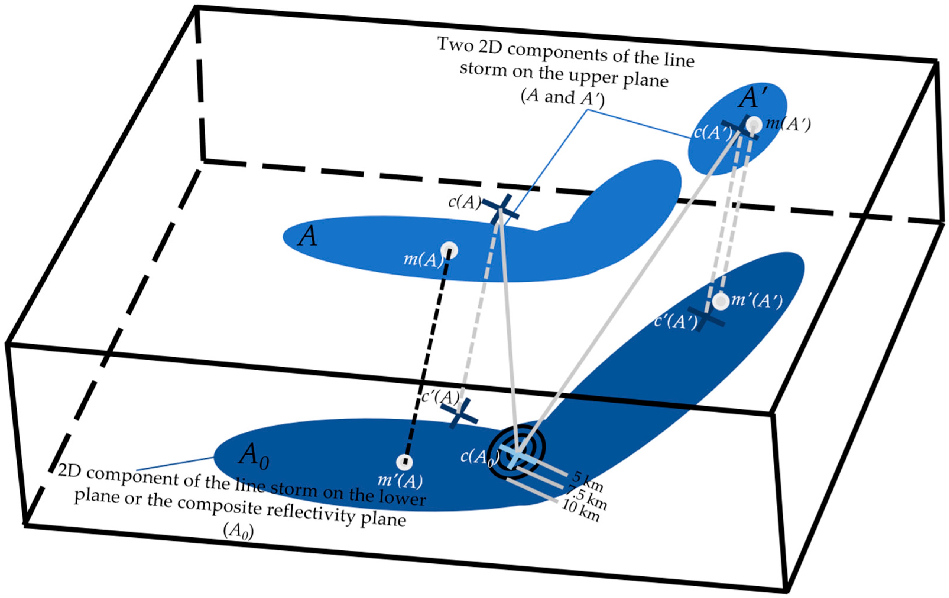
  • Identification of the 3D convective systems and valid point projection method
The identification of convective systems in the modified SCIT can be simplified into three stages: (1) 1D storm segment identification; (2) 2D storm component combination and 2D feature core extraction; and (3) 3D convective system construction. The identification stages are described as follows. In the first stage, storm segments are determined as contiguous sequences of grids whose reflectivity exceeds the specified reflectivity thresholds of 30 and 35 dBZ (denoted by REFLECTIVITY 1–2). DROPOUT COUNT (default = 2) consecutive grid points not more than DROPOUT REF DIFF (default = 5 dBZ) below REFLECTIVITY are also allowed when searching for consecutive grids above REFLECTIVITY. A storm segment is saved if its grid length is greater than SEGMENT LENGTH 1–2 (default = 1.9 km). In the second stage, same-reflectivity thresholded storm segments that are close to one another on the same plane are combined as corresponding REFLECTIVITY components when SEGMENT SEPARATION (default = 0.75 km) and SEGMENT OVERLAP (default = 2) are satisfied. A REFLECTIVITY component must have at least NUMBER OF SEGMENTS (default = 2) segments and an area larger than COMPONENT AREA (default = 10 km2). According to the following condition, that is, whether the centroid of a higher-reflectivity thresholded component falls within the area of a lower-reflectivity thresholded component (i.e., there is an overlapping area between the components), we gradually extract the strongest component from a group of REFLECTIVITY thresholded components in the same plane as the core component of the storm on the plane. The component centroid is calculated based on the component reflectivity weights [2,3]. However, in the third stage, the reduction from the original seven reflectivity thresholds (30, 35, 40, 45, 50, 55, and 60 dBZ) used in the original SCIT to the two reflectivity thresholds (30 and 35 dBZ) used in the modified SCIT poses a problem: the original vertical association method, which is suitable for individual cells (boundary reflectivity values of at least 40–50 dBZ), is no longer adaptable to larger convective storms (boundary reflectivity values of 30–40 dBZ). The boundary reflectivity values of the above two storm scales are based on the work of Dixon and Wiener (1993) [20]. The two main limitations of the original vertical association method are as follows.
The search radius limitation used in the original vertical association method is a dominant factor that cannot be applied to the modified SCIT. As the original SCIT algorithm identifies 3D storm cells with the most intense reflectivity areas, the horizontal distances between the 2D component centroids used to connect the storm cell components in the vertical direction are generally within the three radii of 5, 7.5, and 10 km. Conversely, all sub-storms (i.e., the different cells inside a multi-cell storm) in a large multi-cell storm together determine the storm component 2D centroid on the same plane, and the mass and position difference between the components of these sub-storms in the same plane further affects the position distribution of its 2D centroid. The component mass is an estimate (based on its reflectivity) of the component’s equivalent liquid water content [2]. Therefore, the 2D centroids of some components in a large multi-cell storm may not lie horizontally within the maximum search radius (10 km) of one another. As shown in Figure 2, for the hypothesis of a line storm, the two adjacent-plane components of the line storm are identified by the modified SCIT. The 2D centroid of the upper-plane line storm’s Component A is denoted by c(A), the 2D centroid of the lower-plane line storm’s Component A0 is denoted by c(A0), and the projection point of c(A) on the lower plane is c’(A). When this original vertical association method is employed in the line storm, the projection point c’(A) of Centroid c(A) does not fall within the three circles centered on Centroid c(A0). This attempt at a vertical association between Component A and Component A0, thus, fails. The same failure association also occurs between the upper-plane Component A’ and Component A0.
A secondary factor that cannot be applied to multi-cell storms is that a storm cell in the original vertical association method retains only a maximum mass-valued component on each plane [2]. For a multi-cell storm with several cells, the echoes of these cells may be connected in some low planes, and when they reach above a higher plane due to differences in the vertical growth among different storm cells, the echoes of some cells gradually form individual new components. These new components with smaller masses are discarded on the higher planes when the original vertical association method is applied [2]. As shown in Figure 2, for Components A and A’ of a line storm in the same upper plane, the mass of Component A is greater than the mass of Component A’. If Components A and A’ on the upper plane can be associated with Component A0 on the adjacent lower plane, in the original method, the more massive Component A is retained while the less massive Component A’ is discarded. Note that, in this example in Figure 2, neither Component A’ nor Component A has a vertical association with Component A0 in the adjacent lower plane.
Based on the above limitations, we propose a new vertical association method named the valid point projection method, as shown in Figure 2. A 2D component of the line in the composite reflectivity plane obtained by the first two identification stages in the modified SCIT algorithm is determined as a Standard Component A0 for the line storm. If Centroid c(A’) on the upper-plane Component A’ falls within the area of the Standard Component A0, the upper-plane Component A’ is also associated. Occasionally, some 2D centroids, such as the horizontal projection position c’(A) of Centroid c(A), may fall outside the area of the corresponding Standard Component A0. However, the maximum reflectivity point m(A) in the area of upper-plane Component A must fall within the area of Standard Component A0. The condition parameter of the maximum reflectivity position is introduced to better address the vertical association problem. Finally, Components A’ and A on the same upper plane are associated with the standard component A0. In this work, there are two valid points in the valid point projection method: the 2D centroid point and the 2D maximum reflectivity point of the same component.
Once the above vertical association process is completed, a group of 30 or 35 dBZ thresholded components on different planes with vertical correlations is used to define a 3D convective system. Based on the definition of a storm cell in the original SCIT, a 3D convective system requires not only that the component area on each plane meets certain size and intensity criteria but also that its depth meets the associated criteria [2,11]. For example, if a component area has a maximum reflectivity of at least 30 dBZ and a 30 dBZ area of at least 5 km2 on each plane, a component meets the size and intensity criteria on at least two consecutive planes. However, the original depth criteria do not consider that the small vertical gap between adjacent planes in this paper is only 500 m below the height of 6 km and only 1000 m above the height of 7 km; furthermore, the scan strategy of the SPOL radar also has a poor echo continuity when observing in a sparse radar scan space [21]. As a result, if the original depth criteria are still used, chaff, ground clutter, and “weak convective”areas produced by uneven radar sampling will be identified. A weak convective area usually represents an individual cell with weak vertical growth, which is actually part of a convective system but is separated due to the influence of radar sampling. If the weak convective area is identified, it could interfere with the tracking of the convective system. In this work, the depth criteria still adopt the “DEPTH DELETE” threshold (default 4 km, range between 2 and 4 km) used in the original SCIT algorithm [2], in order to exclude the abovementioned false echoes. Note that 4 km is not a perfect depth threshold, as some storm cells that are farther away and have weak vertical growth may be missed. Additionally, the modified SCIT algorithm identifies isolated convective systems based on their projection echoes in the composite reflectivity plane, and so these thresholds used to distinguish cells close together in a multi-cell storm are not required in the modified SCIT algorithm. The definitions and thresholds of the parameters specified above and used in the modified SCIT algorithm can be found in Appendix A.
The centroid of a 3D convective system is determined from the average of the centroid positions of all the components of a convective system, and its position is represented by a pair of longitude and latitude coordinates. In addition, in the same way as in the original SCIT algorithm [2], other structural characteristic parameters of the convective system are derived in this work (Table 4), including the height of its center of mass, its top (or base)—that is, the value of the maximum echo top height among all grids in the components on the highest (or the lowest) plane of the convective system—its maximum reflectivity (i.e., the maximum reflectivity of all components within the convective storm), the height of its maximum reflectivity (i.e., the height of the component of its maximum reflectivity), and its VIL (which has a strong relationship with the magnitude and depth of the reflectivity). Note that the echo top height mosaic data are used to count the convective system top observed by radars.

2.3.2. Production of Microphysical Characteristics of Convective Systems

Based on the above steps, a 3D convective system with a body structure and a reflectivity boundary of 30 or 35 dBZ can be acquired. According to the number statistics of RH and GR grids within the components of the 3D convective systems identified by the modified SCIT, the microphysical characteristics that are related to the area and height of hail and graupel can be obtained. The hail (or graupel) area on each plane is the number of RH (or GR) grids multiplied by the grid area resolution (0.25 km2). The convective system microphysical characteristic parameters are listed in Table 4, including the height of the maximum hail area (i.e., the height of the plane with maximum RH area in all planes of the convective system), the maximum area of hail (i.e., the maximum RH area in all planes within the convective system), the hail top (or base)—that is, the height of the highest plane (the lowest plane) where RH is present within the convective system— the total area of hail (i.e., the sum of the RH areas on all planes of the convective system), and the total area of hail below the melting layer (i.e., the sum of the RH areas on these planes below the melting layer height within the convective system). The definitions of the graupel characteristic parameters are defined similarly to those for hail.

2.3.3. Tracking and Forecasting Methodology for Convective Systems

The centroid tracking technique used in the original SCIT calculates the motion vector of the storm cell based on the reflectivity-weighted storm centroid displacement and then uses storm centroids from past consecutive radar scans to perform extrapolation forecasting operations with a linear regression technique [2]. In this work, the above tracking method is still applied to the modified SCIT algorithm. The definitions of the tracking characteristic parameters of the convective systems can be found in [2] and are listed in Table 4. The forecast duration is 1 h, including a total of 10 radar volume scans for the SPOL radar.
However, the above tracking method is more suitable for individual cells with a single core than lines or clusters with a large projected area and more cores [2]. This is because the shape of a large convective system may change significantly with time, with mergers and splits into lines or clusters, such that its centroid position may markedly deviate from the originally fitted direction of the storm motion at the next volume scan, causing consecutive tracking of the same convective system to be interrupted. In this case, both newly merged convective systems and newly split convective systems at the most current radar scan are defined as newly formed convective systems with a new ID number.

2.4. The Original SCIT Algorithm and Cell Matching Method

Storm cells are identified by the original SCIT algorithm using mosaic data. Based on the number statistics of RH grids within the components of a 3D storm cell, if the component contains at least one RH grid, the height of the component is saved. After all components in the storm cell are counted, the height range of the RH distribution in the storm cell is obtained. If all components in the storm cell do not contain the RH grids, the storm cell is denoted as a non-hail cell. In the original SCIT using mosaic reflectivity and HC data, the thresholds are the same as in the original SCIT algorithm using volumetric reflectivity data [2], except for the relevant elevation and azimuth thresholds, with reference to the modified SCIT algorithm. The structural and microphysical characteristics of storm cells are listed in Table 4, where the structural characteristics are the same as for the original SCIT using volumetric data [2], and the microphysical characteristics are statistical only for hail, including hail cell number (i.e., the number of hail cells in the convective system), and hail top (or base); that is, the height of the highest (lowest) plane where the component contains at least one RH grid within the hail cell.
For a large convective system, hail is generally distributed in areas of threatening weather with a storm cell. To further determine the positions and characteristics of these hail cells within the convective system in real time, a cell matching method is proposed based on the valid point projection method. In this method, the centroids of storm cells are employed and are projected in the standard component of the convective system on the composite reflectivity plane identified by the modified SCIT; if the centroid of the cell falls within the area of the standard component, the cell is associated with the convective system. Generally, the success rate of cell matching is 100%.

2.5. Production of Mesocyclone Characteristics and Mesocyclone Matching Method

Mesocyclones and their characteristics are obtained by the NSSL-MDA algorithm. Considering that the NSSL-MDA algorithm ignores some shallow mesocyclones far away from the radar, due to the rough vertical sampling of the SPOL radar scan strategy [21], in this work, the mesocyclones only need to consist of two or more shears at consecutive elevation angles (e.g., Weather Surveillance Radar-1988 Doppler Build 9.0 Mesocyclone Algorithm; [9]).
The use of the radar volume scan data in the NSSL-MDA algorithm, as opposed to the radar 3D mosaic data used in the modified SCIT and the original SCIT, first requires conversion of the azimuth–range center of the mesocyclone to its latitude–longitude center. However, we do not modify the remaining mesocyclone characteristic parameters (the definitions of these mesocyclone characteristic parameters in Table 4 can be found in [9]). Note that the mesocyclone’s total depth is calculated by adding the half-power beamwidth to both the top and base of the 3D feature [9].
A mesocyclone matching method is also proposed based on the valid point projection method; that is, the mesocyclone centers are employed and are projected in the standard component of the convective system on the composite reflectivity plane identified by the modified SCIT. If a mesocyclone center falls within the area of the standard component, the mesocyclone is associated with the convective system.
Note that the updraft of the mesocyclone produces weak echo regions, and so it remains to be considered whether the projection points of these mesocyclone centers can all fall within the corresponding standard components with a 30 or 35 dBZ reflectivity boundary. A total of 307 mesocyclones output by the NSSL-MDA algorithm (in Table 2) were position-matched and verified with the convective systems identified by the modified SCIT algorithm. We calculated the relationship between the center positions of these 307 mesocyclones and their corresponding composite reflectivity values and found that 301 of them had a composite reflectivity above 35 dBZ, while the remaining 6 had a composite reflectivity of just above 30 dBZ. In short, the convective systems identified by the modified SCIT algorithm can be associated with almost all mesocyclones.

2.6. ICCE and Convective Characteristic Parameters

Based on the above methods, the ICCE algorithm is proposed; its flowchart is shown in Figure 3. The new storm characteristics calculated by the ICCE algorithm comprise four parts: structural, tracking, mesocyclone, and microphysical characteristic parameters (see Table 4). The latter two characteristics are newly added. The ICCE method includes the use of the modified SCIT algorithm to calculate convective system structure, tracking, and microphysics characteristics in consecutive radar volume scans; the use of the original SCIT algorithm to obtain the structural and microphysical characteristics of hail and non-hail cells within each convective system in real time; and the use of the NSSL-MDA algorithm to determine the mesocyclone characteristics within the convective systems in real time. When the tracking process is complete, the new storm characteristics of the convective systems are sorted as a time series, and the temporal variations of the characteristics during the generation and extinction of the convective system can then be studied.

3. Results

3.1. Algorithm Performance Evaluation

3.1.1. Identification and Matching Results

Figure 4a shows a composite reflectivity image of a hailstorm event (2130 LST 26 April 2019), and the corresponding identification results from the original SCIT and the modified SCIT algorithms are shown in Figure 4b. One large and several non-adjacent small convective systems can be seen to the north of the radar station in this image. These spatially continuous and interconnected pixel regions, labeled from “1” to “10”, represent projected areas of the above non-adjacent convective systems identified by the modified SCIT algorithm. The label numbers of the 10 convective systems are sorted by their VIL in decreasing order. According to the number of identified cells in each convective system, the two convective systems labeled as “1” and “2” are classified as multi-cell storms, and the rest are classified as single-cell storms (Figure 4b). The green and blue outlines in the pixel regions of the 10 convective systems represent the boundaries of non-hail and hail cells identified by the original SCIT algorithm, respectively. In addition, a total of two mesocyclones occurred in the current radar volume scan, and their centers fell within the pixel regions of Convective System 1. For the large Convective System 1, composed of four connected pixel regions, a total number of 20 storm cells and two mesocyclones were identified within it, and 12 hail cells were also included in these 20 storm cells.
As with the original SCIT algorithm, no false alarms occurred in the chaff or ground clutter when the modified SCIT was applied. The 4 km storm depth threshold of the two algorithms eliminated a majority of these potential false alarms. However, some cells with weak vertical growth—such as decaying or newly formed cells—were missed. For example, as shown in Figure 4a, some shallow convective systems (denoted by black ovals) were not identified by either the original SCIT or the modified SCIT in Figure 4b.
For a higher (7 km) altitude plane, Figure 5 shows the identified areas of Convective Systems 1–10 and the distribution of RH and GR within the above areas at 2130 LST. The identified reflectivity areas and HC areas from the original SCIT and the modified SCIT are shown in Figure 5c,d, while Figure 5a,b show the corresponding real reflectivity and HC figures. Comparing Figure 5c to Figure 5a, the areas of several cells belonging to the large Convective System 1 were preserved by the modified SCIT algorithm, instead of only retaining the largest-mass one, as with the original SCIT algorithm. In addition, by comparing the HC areas in Figure 5b,d, we can see that the HC areas identified by the modified SCIT algorithm contained all areas of RH and GR in the plane, but the areas of the cells (within the areas of the blue or green outlines) identified by the original SCIT algorithm contained only part of the RH and GR regions within the convective systems. Therefore, the modified SCIT algorithm essentially meets its algorithm design requirements for the acquisition of 3D convective system echo structures, the matching of cells and mesocyclones with the convective systems, and the distribution of hail and graupel in the convective systems.

3.1.2. Tracking Results

Figure 6 shows the past trajectories and future motion directions of the identified convective systems and matched mesocyclones at 2130 LST. These convective systems, labeled 1–10, except for Convective Systems 8 and 9—which were identified for the first time—had existed for more than two radar volume scans. Convective System 8 was newly formed at the current radar volume scan, while Convective System 9 had detached from Convective System 1 in the last radar volume scan (6 min ago). The remaining convective systems were identified after meeting the algorithm’s size, intensity, and depth criteria and were tracked to the current radar volume scan.
Convective System 1 entered the radar observation field from the northwest corner of the Guangzhou radar and was first identified at 1736 LST. Later, while the larger echo area of Convective System 1 entered the radar observation field, Convective System 1 was also tracked continuously until 2130 LST. During this period, there were no remarkable mergers or splits and, thus, no obvious shift of the centroid of Convective System 1 between adjacent radar volume scans, enabling consecutive tracking of the Convective System 1. However, tracking of this Convective System 1 was stopped at 2136 LST due to its splitting into two reflectivity areas. The two areas also represented two newly formed convective systems, whose centroid positions were 35 km and 102 km away from the centroid position of the unsplit Convective System 1 at 2130 LST. A similar situation may also occur in a merger between two or more large convective systems, which is not discussed here. In addition, the remaining smaller Convective Systems 2–9 were able to achieve continuous tracking from post-primary to pre-dissipation.
Figure 7 depicts the temporal variation of the number of both storm cells (Figure 7a) and mesocyclones (Figure 7b) within Convective System 1 from 1736 to 2130 LST. As shown in Figure 7a, the total number of cells increased as more areas of Convective System 1 came into the radar observation field. Among these storm cells, more than three-quarters of the cells were hail cells, distributed in the areas with the most intense reflectivity in Convective System 1 (Figure 4b). The generation and death of storm cells in Convective System 1 were very frequent. For Convective System 1, in each radar volume scan, several newly formed cells in Convective System 1 were detected for the first time, while the decaying or dissipated cells disappeared into the detection target of the original SCIT algorithm. During the movement of Convective System 1, it often occurred that nearby small cells also merged into Convective System 1, but this merging did not change the shape of Convective System 1 significantly and, thus, had no adverse effect on the tracking of Convective System 1. Additionally, as shown in Figure 7b, the change of mesocyclones in different cell areas within Convective System 1 was relatively rapid. A total of five mesocyclones formed, four of which decayed and disappeared during this period. From the above analysis, if the shape of a large convective system does not change sharply in adjacent time steps, the rapid evolution of both storm cells and mesocyclones within the convective system can be expected to have no adverse effect on the tracking of the convective system.

3.2. Advantages of ICCE Products in Observing Hailstorm Evolution

The Guangzhou radar collected data for the complete evolution process of the hailstorm that occurred from 1248 to 1948 LST on 11 April 2019 (see Table 2). The development process of the hailstorm’s echo shape is shown in Figure 8. The hailstorm started with a single-cell storm at 1248 LST, then matured at 1342 LST and faded into a cluster storm at 1400 LST, finally grew into a supercell at 1518 LST, and moved out of the radar’s vision at 1948 LST.
The corresponding evolution process of some new storm characteristics of the hailstorm is depicted in Figure 9. The hailstorm formed in the mountainous area of Northern Zhaoqing at around 1248 LST. At the time of this radar volume scan, the hailstorm had not been detected, as it did not yet meet the modified SCIT algorithm’s convective system definition rules, and neither hail nor graupel was found in the hailstorm. Six minutes later, at 1254 LST, when the hailstorm was detected for the first time as a single-cell storm, an average graupel area of about 2 km2 had just appeared in the single-cell storm (Figure 9b). Twelve minutes later, at 1306 LST, about 4 km2 of hail regions appeared above the melting layer (Figure 9c), accompanied by a further increase in the hailstorm’s maximum reflectivity (Figure 9e). Until nearly 1342 LST, the maximum reflectivity, echo top, and VIL of the single-cell storm reached their peak values of 68 dBZ, 12 km, and 43 kg/m2 (Figure 9e), respectively, indicating that the single-cell storm had entered a mature stage. Meanwhile, the height of the maximum graupel area (about 250 km2) of the single-cell storm also rose above the height of the −20 °C environment temperature (Figure 9b). During the following period, from 1348 to 1406 LST, larger areas of hail (about 180 km2) and graupel (about 400 km2) regions were found in the environment with temperatures ranging from 0 to −20 °C (Figure 9b,c). Correspondingly, the total area of graupel and hail regions also increased to their respective maximum values (Figure 9e). These features suggest that a large amount of graupel accumulated in the upper part of the hailstorm (above the height of the −20 °C environment temperature) during the growth of the hailstorm. After the hailstorm matured and stopped growing, a large amount of graupel fell from the upper part of the hailstorm, which promoted the production of larger areas of graupel and hail in the following time. Additionally, we speculate that the movement of the single-cell storm along the complicated mountainous terrain from 1254 to 1348 LST may have played a leading role in its formation and development (Figure 8a).
After 1342 LST, the single-cell storm faded into a cluster storm at 1354 LST, accompanied by a rapid decrease in the hailstorm’s maximum reflectivity, echo top, and VIL values (Figure 9e). However, from the first appearance of Mesocyclone 1 (its center position is indicated by an orange cross in Figure 8a) at 1406 LST to its development to its strongest state at 1430 LST, the total mesocyclone depth increased from 4 to 6.5 km, and the maximum rotational velocity of Mesocyclone 1 also rose from 13 to 16 m/s (Figure 9d), while the echo top and VIL of the cluster rose again rapidly (Figure 9a,e). When the echo top and VIL of the cluster rose to their highest points and peaked at 1418 LST, the downward trend in the total area of graupel and hail regions halted and started to increase again (Figure 9e). In addition, unlike the phenomenal growth of the cluster’s VIL and echo top values, the maximum reflectivity value of the cluster storm was above 60 dBZ and remained steady from 1406 to 1418 LST (Figure 9e), while the top height of the maximum reflectivity value increased from 6 to 9 km (Figure 9a). The above features suggest that the emergence and further development of mesocyclones will not only reinforce weakened storms but also slow down the reduction of the area of hail and graupel in mature storms for a short period, causing them to grow again.
Subsequently, a newly formed mesocyclone appeared in each of three consecutive radar volume scans at 1442, 1448, and 1454 LST. The three new mesocyclones are Mesocyclones 2–4 in Figure 8a, and all of these mesocyclones (including Mesocyclone 1) first appeared in the middle troposphere (Figure 9d). Although multiple mesocyclones appeared in the cluster after 1442 LST, Mesocyclones 1 and 2 weakened and dissipated at 1454 LST, the cells in the middle and rear of the cluster (relative to the cluster storm motion) also synchronously entered their dissipating and splitting stages and eventually disappeared at 1524 LST. As a result, the large area of graupel produced by the strengthening of the cluster by Mesocyclone 1 declined rapidly from 1448 to 1506 LST, and the total area of hail remained at a low point after 1454 LST before supercell formation (Figure 9e).
After 1454 LST, the subsequent development of the cluster was driven by two mesocyclone-producing cells in the front of the cluster (Figure 8d). The cell where Mesocyclone 3 was located and the other cell where Mesocyclone 4 was located gradually approached at 1500 LST and merged between 1506 and 1512 LST (Figure 9d). The merged Mesocyclone 4 eventually promoted the development of the cell, which was located into a supercell at 1518 LST (Figure 8e). As shown in Figure 8e, at 1518 LST, a typical hook echo—which is a supercell signature—formed at low levels, and a weak shear was first observed at the lowest elevation (0.5°). From 1454 to 1518 LST, the maximum reflectivity, echo top, and VIL values of the supercell increased again, concurrent with the changes seen in the total area of hail, but the total area of graupel stopped decreasing after 1506 LST and remained stable (Figure 9e). This phenomenon was associated with the decay and dissipation of Mesocyclones 1 and 2 in the rear and middle of the cluster storm and the formation and development of Mesocyclones 3 and 4 in the front of the cluster storm. While the low-level rotational velocity of Mesocyclone 4 further increased after 1518 LST, the height of the maximum rotational velocity of Mesocyclone 4 gradually shifted from the middle troposphere (~5 km) to the surface layer (~0.5 km) and finally reached the lowest elevation layer at 1600 LST (Figure 9d). In this process, the areas of graupel and hail regions (including their total areas, the hail regions below the melting layer, and the graupel regions above the −20 °C environment temperature) began to increase rapidly when the hook echo formed (Figure 9b,c), accompanied by a further increase in the values of the supercell’s maximum reflectivity, echo top, and VIL (Figure 9e). After the maximum rotational velocity of Mesocyclone 4 first peaked between 1536 and 1542 LST (Figure 9d), the maximum reflectivity, echo top, and VIL of the supercell also reached their maximum values at 1548 LST (Figure 9e). As shown in Figure 8f, at 1542 LST, a hook echo and a radial velocity couplet were obvious at the height of ~1 km, meaning that a mature supercell had appeared. Although the maximum rotational velocity of Mesocyclone 4 began to decrease slowly thereafter, the height of the maximum rotational velocity of Mesocyclone 4 was constantly approaching the ground, which could further transport the abundant water vapor on the ground to above the melting layer and provide conditions for the further growth of hail and graupel (Figure 9d). After 1606 LST, the weak mesocyclone on the lowest elevation layer declined to a weak shear (Figure 9d), and the total area of hail did not continue to increase, reaching its maximum value at 1612 LST (Figure 9e). Furthermore, weak mesocyclones existing in the height range of 3–6 km after 1600 LST could still promote the growth of graupel regions, and the reduction of the total mesocyclone depth at 1618 LST finally caused the maximum total area of graupel to appear at 1624 LST (Figure 9b). After 1612 LST, the total depth of Mesocyclone 4 rapidly decreased (Figure 9d), accompanied by a decrease in the areas of graupel and hail, as well as decreases in the maximum reflectivity and VIL of the supercell (Figure 9e). Hereafter, the surface observation stations near the hailstorm trajectory also observed strong surface winds of above 14 m/s and hail events (Figure 9f and Table 3). The hailfall positions of ground-based observations from 1600 to 1630 LST are shown at points B, C, and D (denoted by solid black circles) in Figure 8a. These features indicate that the weakening Mesocyclone 4 in the mature supercell was accompanied by the occurrence of hail and gale on the ground, and the rapid fall of big raindrops and hailstones promoted further decay of the supercell. A similar situation occurred after Mesocyclone 4 in the supercell strengthened again at 1642 LST.
In addition, as shown in Figure 9f, the moving speed of the hailstorm increased rapidly after the hailstorm formed, first reaching the 14 km/h peak in the single-cell storm stage at 1354 LST after the single-cell storm had matured. Subsequently, its moving speed slowly decreased with the weakening of the hailstorm from a peak of over 14 km/h at 1354 LST to approximately 12 km/h at 1454 LST. Eventually, with the formation of the supercell, its moving speed increased rapidly again to over 15 km/h, which was maintained throughout the supercell stage.
From the trends of the new storm characteristics, several findings were obtained: First, the tendencies of the maximum reflectivity, echo top, and VIL of the hailstorm were inconsistent with the area variation of hail and graupel within the hailstorm but were in good agreement with the development of matched Mesocyclones 1–4. In general, the emergence and rapid enhancement of a mesocyclone increased synchronously with the maximum reflectivity, echo top, and VIL of the hailstorm in which the mesocyclone is located. When the mesocyclone reached a peak, the peak of the hailstorm’s maximum reflectivity, echo top, and VIL followed, and after the peak of the mesocyclone, the hailstorm’s maximum reflectivity, echo top, and VIL tended to decrease. In addition, the continual growth of hail and graupel regions was associated with mesocyclone development. After the mesocyclone peak, the area of hail and graupel regions continued to increase or remained steady until the weakened mesocyclone fell to a low point or disappeared. For the supercell, however, the arrival of weak shear at the lowest elevation layer allowed the area of hail to reach its peak in advance. Second, the height of the maximum graupel area above the height of the −20 °C environment temperature may be a sign that the areas of graupel and hail are about to reach their peaks, indicating the occurrence of hailfall and gale on the ground in the subsequent time. Third, short-lived mesocyclones can promote the growth of graupel but not greatly increase the area of hail. Fourth, the movement of a mature storm will be faster, and a supercell will move faster (≥15 km/h) than a non-supercell.

4. Discussion

Although the ICCE algorithm was able to identify, characterize, track, and forecast the movement of convective systems, there are still some points where the ICCE algorithm needs to be improved in the future. For example,
(1)
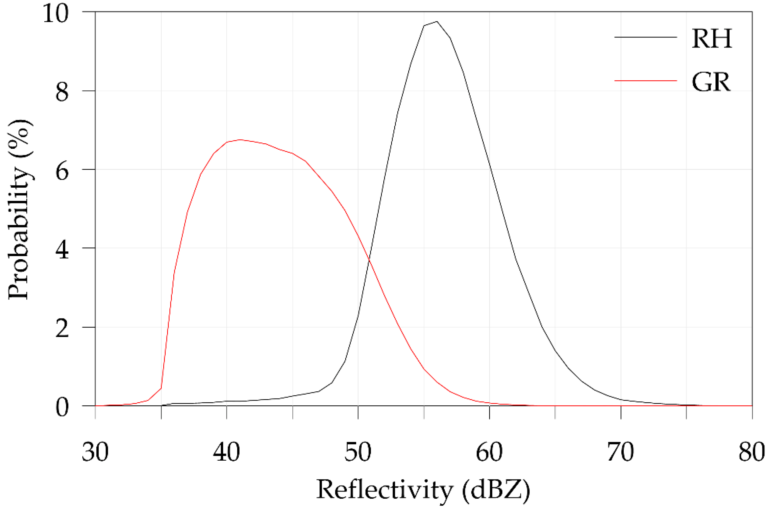
The determination of the identification thresholds used in the modified SCIT algorithm. The threshold, chosen in this paper to be 30 and 35 dBZ, was obtained statistically from the reflectivity of hail and graupel output by the HC algorithm. As the HC algorithm is based on a statistical fuzzy logic approach, it does not directly observe the hydrometeors within the convective system and, therefore, still differs from reality. The involvement of other dual-polarization radar parameters (e.g., ZDR, KDP, and ρhv), in addition to the already existing reflectivity (i.e., Z), may still be required in future recognition identification thresholds.
(2)
The optimization of the convective system tracking algorithm. The tracking algorithm of convective systems used in the modified SCIT algorithm in this paper still adopts the centroid tracking algorithm used in the original SCIT algorithm proposed by Johnson et al. [2], which may lead to tracking interruptions with the splitting and merging of some large convective systems, and a better tracking method may be established in the future by referring to the tracking advantages of the Tracking Radar Echoes by Correlation algorithm [2] for large-scale echoes.

5. Conclusions

At present, the dual-polarization radars in China still use a hail nowcasting system with low detection accuracy and poor forecast precision based on structural storm characteristics obtained from radar reflectivity measurements. To further improve the nowcasting capability by applying HC data (storm microphysics) and mesocyclone data (storm dynamic) provided by a dual-polarization radar platform, in this paper, we propose the ICCE algorithm for dual-polarization radars based on the SCIT algorithm [2], the NSSL-MDA algorithm [9], and the HC algorithm [7]. The ICCE algorithm can simultaneously extract structural, tracking, microphysical, and mesocyclone characteristics of hailstorms for each radar volume scan, which can then be used to study the temporal evolution of the characteristics of the convective system for its initial generation until its extinction and, furthermore, allows us to obtain the relationships between these characteristics from the ICCE, which is ultimately expected to help in improving hail and gale nowcasting capabilities; for example, when certain correlations are obtained statistically for the abovementioned characteristics to forecast the specific hailfall point and the accurate time of occurrence of hailfall and gales in the future convective system.
The ICCE algorithm is composed of three parts:
(1)
The modified SCIT: Based on the original SCIT algorithm using mosaic reflectivity data, we propose a modified SCIT algorithm, which is better able to identify and track convective systems and their hail and graupel after selecting reflectivity thresholds determined based on reflectivity factor with hail and graupel statistics, establishing a 3D convective system with a complete structure of the main body based on the valid point projection method. Furthermore, we introduce the HC data to increase the characteristic parameters of the area and height of hail and graupel and track the convective system using the centroid tracking method of the original SCIT algorithm.
(2)
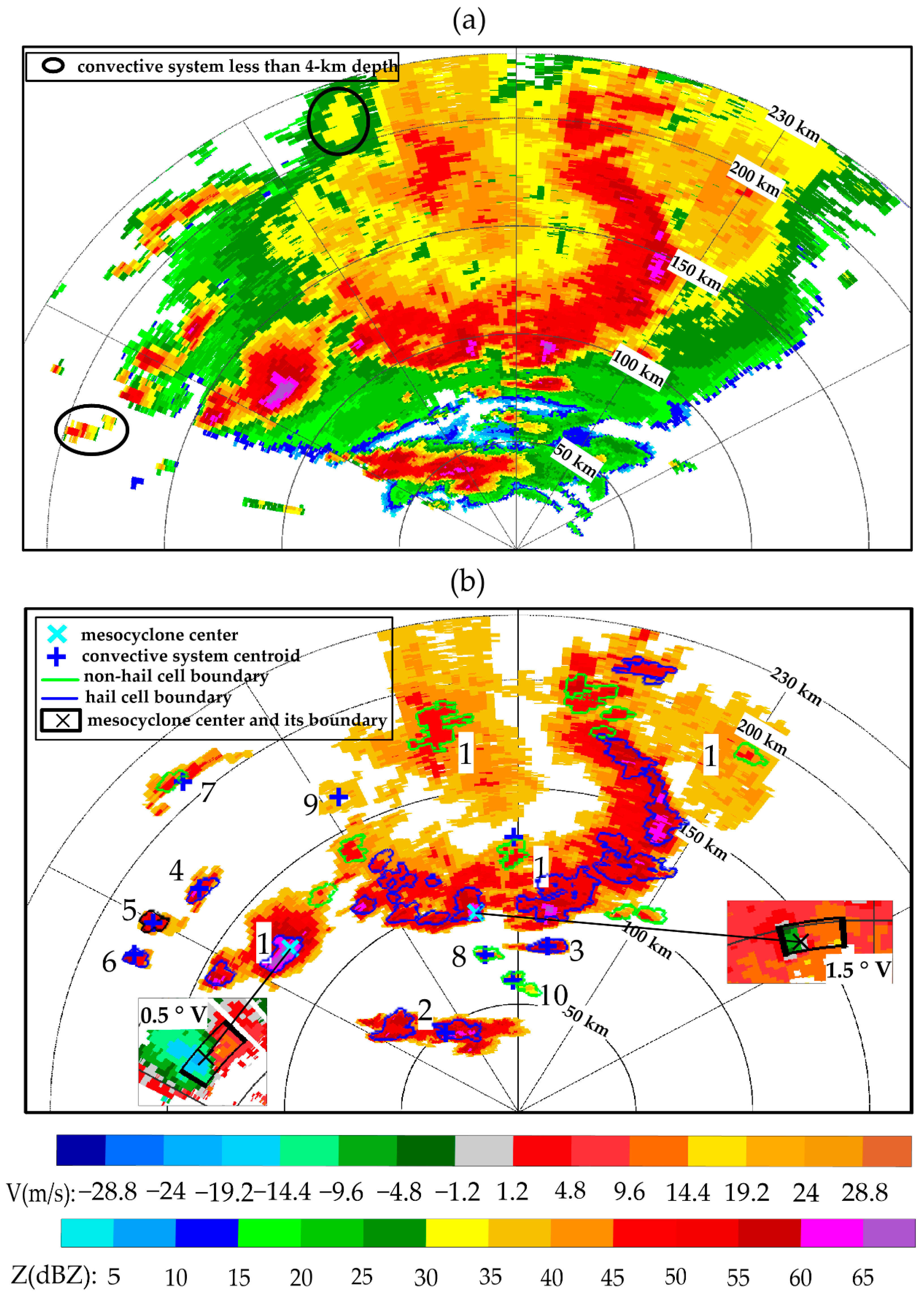
The original SCIT and cell matching: Based on the original SCIT algorithm using mosaic reflectivity data, we add hail characteristics to the original SCIT algorithm, which can allow for distinguishing between hail and non-hail cells by introducing HC data and obtaining the height range of the hail distribution of the hail cell, in addition to its structural characteristics. To study the local variability of characteristics within convective systems (especially large line storms and cluster storms), a cell-matching method is also used in this paper in order to localize storm cells.
(3)
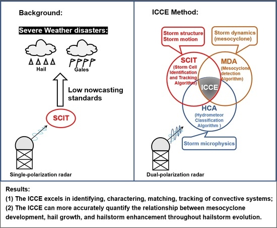
NSSL-MDA and mesocyclone matching. Based on the NSSL-MDA algorithm proposed by Stumpf et al. (1998) [9], we lowered some of the parameter thresholds of the algorithm to obtain more mesocyclones and larger updraft velocity, and a mesocyclone matching method was also applied to mesocyclone localization in order to obtain the dynamical characteristics of the convective system.
Using the above algorithms, we compared the differences between the modified SCIT and the original SCIT in terms of identified storm structure and hail−graupel completeness, considering a large line storm and several small convective systems, as well as individual tests of the tracking of this large line storm and the matching of cells and mesocyclones with the line storm. The results demonstrated that the modified SCIT algorithm is adequate for identifying 3D convective systems with a main body of echoes and containing a relatively complete hail and graupel areas, while the position-matching method enables real-time characterization of storm cells and mesocyclones within convective systems. In addition, the modified SCIT algorithm is more effective in tracking convective systems with insignificant morphological changes.
Furthermore, an example of a hailstorm evolving into a supercell was used to demonstrate the benefits of the ICCE algorithm, and ground-based observations and the output of the ICCE were utilized to analyze the relationship between storm characteristic parameters and gale and hailfall events during the process. The results indicated that mesocyclones are instrumental in both the development of the storm and the growth of hail and graupel. The tendency of structural storm characteristics is essentially consistent with mesocyclone development, but the temporal trends of the area of hail and graupel have a temporal delay when compared to the changes in storm structural and mesocyclone characteristics. In particular, after mesocyclones reach their peak (and do not dissipate in the subsequent period), the total area of hail (or graupel) may still increase or remain stable (rather than decreasing as rapidly as the structural storm characteristics) throughout the period, and the hailfall and gales are also more frequent during the period. Consequently, the ICCE outputs more clearly indicate the relationships between storm evolution, hail production, and mesocyclone development.

Author Contributions

Conceptualization, C.W. (Chong Wu) and L.L.; methodology, C.W. (Chao Wang); software, C.W. (Chao Wang); validation, C.W. (Chao Wang), C.W. (Chong Wu) and L.L.; formal analysis, C.W. (Chong Wu); investigation, C.W. (Chao Wang); resources, L.L.; data curation, C.W. (Chao Wang); writing—original draft preparation, C.W. (Chao Wang); writing—review and editing, C.W. (Chao Wang); visualization, C.W. (Chao Wang); supervision, C.W. (Chong Wu); project administration, L.L.; funding acquisition, C.W. (Chao Wang) and L.L. All authors have read and agreed to the published version of the manuscript.

Funding

This research was funded by the National Natural Science Foundation of China (Grant No. U2142210), the Postgraduate Research & Practice Innovation Program of Jiangsu Province (Grant No. KYCX20_0918) and the Basic Research Fund of CAMS(Grant No. 2021Z012).

Data Availability Statement

Not applicable.

Conflicts of Interest

The authors declare no conflict of interest.

Appendix A

Based on the parameter settings in the original SCIT algorithm proposed by Johnson et al. (1998) [2], the following parameters and thresholds were applied to the modified SCIT algorithm to identify convective systems.
(1)
COMPONENT AREA 1–2
Definition: Area threshold for features to be considered as convective system components for each of the two reflectivity thresholds (30 and 35 dBZ).
Algorithmic response to change: Lowering this parameter will cause the detection of smaller convective systems, and raising this parameter will decrease the number of detections.
Values: Default 10 km2, range (10.0–30 km2).
(2)
DEPTH DELETE
Definition: Threshold depth is used to filter out strong non-meteorological echoes (chaff and ground clutter) and “weak convective” produced by uneven radar sampling.
Algorithmic response to change: The lowest threshold of the range depends on the vertical gap resolution of the 3D mosaic data, which cannot be less than twice the vertical gap resolution. In general, if a low threshold is used, more shallow convective systems will be identified, while a high threshold will also miss weak convective systems that have the potential to become stronger in the future.
Values: Default 4 km, range (2–4 km).
(3)
DROPOUT COUNT
Definition: Maximum number of contiguous grids with the reflectivity below the threshold REFLECTIVITY by less than or equal to DROPOUT REF DIFF that may be included in a segment identified with REFLECTIVITY.
Algorithmic response to change: Setting this threshold lower will cause stricter adherence to the threshold REFLECTIVITY when building segments. Setting this threshold higher will cause less strict adherence to the threshold REFLECTIVITY when building segments.
Values: Default 2, range (0–5 grids).
(4)
DROPOUT REF DIFF
Definition: The difference in effective reflectivity of sample volumes below REFLECTIVITY that may still be included in a segment identified with REFLECTIVITY.
Algorithmic response to change: Setting this threshold lower will allow less departure from REFLECTIVITY when building a segment. Setting this threshold higher will allow more departure from REFLECTIVITY when building a segment.
Values: Default 5 dBZ, range (0–10 dBZ).
(5)
NUMBER OF SEGMENTS
Definition: Minimum number of segments required to save a 2D component.
Algorithmic response to change: Fewer convective systems are detected at longer ranges when the threshold is set too high. Setting the parameter to one will cause 2D convective system components to be built for clutter.
Values: Default 2, range (1–4).
(6)
REFLECTIVITY 1–2
Definition: The two reflectivity thresholds used for the one-and two-dimensional parts of the convective system building process (30 and 35 dBZ).
Algorithmic response to change: These thresholds do not need to be changed. It is a reflectivity statistic of RH and GR obtained by the Hydrometeor Classification algorithm and is used to obtain the complete distribution of hail and graupel within the convective systems.
Values: Default 30 and 35 dBZ.
(7)
REFLECTIVITY LENGTH 1–2
Definition: Minimum required length of a segment.
Algorithmic response to change: Lowering this parameter will cause the detection of more smaller convective systems, and raising this parameter will decrease the number of detections.
Values: Default 1.9 km, range (1.9–9.9 km).
(8)
SEGMENT SEPARATION
Definition: Maximum segment separation allowed for grouping segments into 2D components.
Algorithmic response to change: In general, there is little effect in increasing the maximum segment separation except where storms are “affected” by blockages. The value of the parameter should never go below the grid resolution of 3D mosaic data, or no storms will be identified.
Values: Default 0.75 km, range (0.75–1.75 km).
(9)
SEGMENT OVERLAP
Definition: Minimum rage overlap required for grouping segments into 2D components.
Algorithmic response to change: This parameter should never be lower than the grid length resolution of mosaic data. The effect of lowering this parameter is unknown at this time. Raising this parameter will cause fewer detection of smaller convective systems and becomes meaningless without a corresponding change in the area thresholds (COMPONENT AREA).
Values: Default 2, range (0–5 grids).

Appendix B

The abbreviations of the main instruments, algorithms, and parameters in this paper are described as follows.
(1)
SPOL
Full name: S-band dual-polarization radar.
(2)
HC
Full name: Hydrometeor Classification (algorithm or data).
Notes: This algorithm, which uses dual-polarization radar base (or mosaic) data, was proposed by Park et al. (2009) [8] and developed and applied to China’s dual-polarization radars by Wu et al. (2018) [7].
(3)
The original SCIT
Full name: the original Storm Cell Identification and Tracking algorithm.
Notes: This algorithm, which uses volumetric reflectivity data, was proposed by Johnson et al. (1998) [2] and applied to the severe weather detection systems of the US WSR-88D radars. Later, the other version of the SCIT algorithm for mosaic data was developed by Yang et al. [11] and applied in China’s new-generation weather radar network. The main body of the two versions is essentially the same, so they are both referred to as the original SCIT.
(4)
The modified SCIT
Full name: the modified Storm Cell Identification and Tracking algorithm.
Notes: This algorithm, which uses mosaic reflectivity, composite reflectivity, and hydrometeor classification (HC) data, is developed in this paper based on the original SCIT algorithm. The advantage of the algorithm is that it not only identifies and tracks the 3D convective system but also studies the temporal evolution of the area and height of hail and graupel within the convective system.
(5)
NSSL-MDA
Full name: The National Severe Storms Laboratory (NSSL) developed an enhancement of the Mesocyclone Detection Algorithm.
Notes: This algorithm, which uses volumetric doppler velocity data, was developed by Stumpf et al. (1998) [9].
(6)
VIL
Full name: Vertically integrated liquid water.
Notes: This parameter is one of the structural characteristics of the storm, which is a strong relationship with the magnitude and depth of the reflectivity of the storm.
(7)
GR
Full name: Graupel.
Notes: This parameter is a microphysical parameter, which is output by the HC algorithm.
(8)
RH
Full name: A mixture of rain and hail.
Notes: This parameter is a microphysical parameter, which is output by the HC algorithm.
(9)
Convective system
Full name: Mesoscale convective system.

References

  1. Kumjian, M.R.; Ryzhkov, A.V. Polarimetric signatures in supercell thunderstorms. J. Appl. Meteorol. Clim. 2008, 47, 1940–1961. [Google Scholar] [CrossRef]
  2. Johnson, J.T.; Mackeen, P.L.; Witt, A.; Mitchell, E.D.W.; Stumpf, G.J.; Eilts, M.D.; Thomas, K.W. The storm cell identification and tracking algorithm: An enhanced WSR-88D algorithm. Weather Forecast. 1998, 13, 263–276. [Google Scholar] [CrossRef]
  3. Han, L.; Fu, S.; Zhao, L.; Zheng, Y.; Wang, H.; Lin, Y. 3D Convective storm identification, tracking, and forecasting—An enhanced TITAN algorithm. J. Atmos. Ocean. Technol. 2010, 26, 719–732. [Google Scholar] [CrossRef]
  4. Wang, P.; Shi, J.; Hou, J.; Hu, Y. The identification of hail storms in the early stage using time series analysis. J. Geophys. Res. Atmos. 2018, 123, 929–947. [Google Scholar] [CrossRef]
  5. Joe, P.; Burgess, D.; Potts, R.; Keenan, T.; Stumpf, G.; Treloar, A. The S2K severe weather detection algorithms and their performance. Weather Forecast. 2004, 19, 43–63. [Google Scholar] [CrossRef]
  6. Witt, A.; Eilts, M.D.; Stumpf, G.J.; Johnson, J.T.; Mitchell, E.D.W.; Thomas, K.W. An enhanced hail detection algorithm for the WSR-88D. Weather Forecast. 1998, 13, 286–303. [Google Scholar] [CrossRef]
  7. Wu, C.; Liu, L.; Wei, M.; Xi, B.; Yu, M. Statistics-based optimization of the polarimetric radar hydrometeor classification algorithm and its application for a squall line in South China. Adv. Atmos. Sci. 2018, 35, 296–316. [Google Scholar] [CrossRef]
  8. Park, H.S.; Ryzhkov, A.V.; Zrnic, D.S.; Kim, K. The hydrometeor classification algorithm for the polarimetric WSR-88D: Description and application to an MCS. Weather Forecast. 2009, 24, 730–748. [Google Scholar] [CrossRef] [Green Version]
  9. Stumpf, G.J.; Witt, A.; Mitchell, E.D.W.; Spencer, P.L.; Johnson, J.T.; Eilts, M.D.; Thomas, K.W.; Burgess, D.W. The national severe storms laboratory mesocyclone detection algorithm for the WSR-88D. Weather Forecast. 1998, 13, 304–326. [Google Scholar] [CrossRef]
  10. Miller, L.J.; Tuttle, J.D.; Knight, C.A. Airflow and hail growth in a severe northern High Plains supercell. J. Atmos. Sci. 1988, 45, 736–762. [Google Scholar] [CrossRef]
  11. Yang, J.; Liu, L.; Li, G.; Wang, G.; He, H. A new technique for storm cell and mesoscale convective systems identification, tracking and nowcasting based on the radar mosaic data. Acta Meteorol. Sin. 2012, 70, 1347–1355. (In Chinese) [Google Scholar] [CrossRef]
  12. Li, G.; Liu, L.; Lian, Z.; Zhou, M.; Li, Z. Statistical study of the identification of thunderstorm gale based on the radar 3D mosaic data. Acta Meteorol. Sin. 2014, 72, 1347–1355. (In Chinese) [Google Scholar] [CrossRef]
  13. Wu, C.; Liu, L.; Liu, X.; Li, G.; Chen, C. Advances in Chinese dual-polarization and phased-array weather radars: Observational analysis of a supercell in southern China. J. Atmos. Ocean. Technol. 2018, 35, 1785–1806. [Google Scholar] [CrossRef]
  14. Johns, R.H.; Doswell, C.A., III. Severe local storms forecasting. Weather Forecast. 1992, 7, 588–612. [Google Scholar] [CrossRef]
  15. Xiao, Y.; Liu, L. Study of methods interpolating data from weather radar network to 3-D grid and mosaics. Acta Meteorol. Sin. 2006, 64, 647–657. (In Chinese) [Google Scholar] [CrossRef]
  16. Wen, L.; Zhao, K.; Zhang, G.; Xue, M.; Zhou, B.; Liu, S.; Chen, X. Statistical characteristics of raindrop size distributions observed in East China during the Asian summer monsoon season using 2-D video disdrometer and micro rain radar data. J. Geophys. Res. Atmos. 2016, 121, 2265–2282. [Google Scholar] [CrossRef] [Green Version]
  17. Ryzhkov, A.V. The impact of beam broadening on the quality of radar polarimetric data. J. Atmos. Ocean. Technol. 2007, 24, 729–744. [Google Scholar] [CrossRef]
  18. Giangrande, S.E.; Krause, J.M.; Ryzhkov, A.V. Automatic designation of the melting layer with a polarimetric prototype of the WSR-88D radar. J. Appl. Meteorol. Clim. 2008, 47, 1354–1364. [Google Scholar] [CrossRef]
  19. He, G.; Li, G.; Zou, X.; Ray, P.S. Applications of a velocity dealiasing scheme to data from the China new generation weather radar system (CINRAD). Weather Forecast. 2012, 27, 218–230. [Google Scholar] [CrossRef]
  20. Dixon, M.; Wiener, G. TITAN: Thunderstorm identification, tracking, analysis and nowcasting—A radar-based methodology. J. Atmos. Ocean. Technol. 1993, 10, 785–797. [Google Scholar] [CrossRef]
  21. Brown, R.A.; Janish, J.M.; Wood, V.T. Impact of WSR-88D scanning strategies on severe storm algorithms. Weather Forecast. 2000, 15, 90–102. [Google Scholar] [CrossRef]
Figure 1. The probability distributions of reflectivity versus the RH and GR output from the HC algorithm.
Remotesensing 15 00808 g001
Figure 2. An example of a line storm under the new and old vertical association methods. Shaded areas (A, A’, and A0) represent the 2D components of the line storm identified by the two reflectivity thresholds of 30 and 35 dBZ. The two components of A and A’ are both on the same upper plane. Component A0 ideally represents the adjacent lower-plane component in the original identification method, while it indicates the composite reflectivity plane standard component in the new identification method. The blue cross points of c(A0), c(A), and c’(A), respectively, refer to the centroid of component A0, the centroid of component A, and its projection point on the plane of component A0. The white solid circle points of m(A) and m’(A) indicate the maximum reflectivity in the area of component A and its projection point on the plane of component A0, respectively. The three black circles of 5, 7.5, and 10 km are the search areas used in the old vertical association method. The indications of these points of c(A’), c’(A’), m(A’), and m’(A’) with respect to component A’ are the same as those of the points associated with component A.
Remotesensing 15 00808 g002
Figure 3. Flowchart describing the Integrated Convective Characteristic Extraction (ICCE) algorithm.
Remotesensing 15 00808 g003
Figure 4. Illustration of differences in the identification results from the original SCIT and the modified SCIT at 2130 LST on 26 April 2019. (a) The real composite reflectivity; the shallow reflectivity echoes inside these black ovals were discarded by the above two algorithms. In (b), the spatially continuous and interconnected pixel regions labeled from “1” to “10” represent the composite reflectivity areas of the 10 non-adjacent convective systems identified by the modified SCIT, while the green and blue outlines inside the 10 convective systems indicate the boundaries of non-hail cells and hail cells identified by the original SCIT, respectively. The two small Doppler velocity figures show the areas (denoted by black rectangles) and center positions (denoted by black crosses) of the two mesocyclones in Convective System 1.
Remotesensing 15 00808 g004
Figure 5. Illustration of differences in the hydrometeor areas in the identification results from the original SCIT and the modified SCIT at 2130 LST on 26 April 2019: (a,c) real and identified reflectivity areas in the 7 km altitude plane (above the melting layer); (b,d) real and identified hydrometeor classification areas at the 7-km altitude plane. In (c,d), the pixel regions identified by the modified SCIT represent the echo areas of Convective Systems 1–10 and their hydrometeor classification results, while green (blue) outlines inside the 10 convective systems indicate the boundaries of non-hail cells (hail cells) identified by the original SCIT.
Remotesensing 15 00808 g005
Figure 6. Centroid tracking trajectory and motion prediction direction of convective systems at 2130 LST on 26 April 2019. Example of centroid tracking failure: Convective System 1, with four reflectivity areas, split into two isolated convective systems at 2136 LST, with new centroids 35 km and 102 km away from the centroid of the current Convective System 1, respectively.
Remotesensing 15 00808 g006
Figure 7. Temporal variation of the number of both storm cells (a) and mesocyclones (b) matching Convective System 1 from 1736 to 2130 LST on 26 April 2019.
Remotesensing 15 00808 g007
Figure 8. Temporal evolution of (a) composite reflectivity echoes of a hailstorm and (bh) four matched mesocyclones observed by the SPOL radar in Guangzhou on 11 April 2019. In (a), gray shading represents the topography, composite reflectivity echoes represent the standard component of the hailstorm identified by the modified SCIT, and red (and blue) outlines represent the projected boundary of matched non-hail (and hail) cells in the hailstorm identified by the original SCIT. (a) also shows the hailstorm centroid trajectory and the matched four mesocyclone center trajectories, as well as the distribution of observational instruments, including an SPOL, an L-band sounding, and several surface observation stations. Note Mesocyclones 1–4 are labelled in order of their appearance. (bh) show several plan position indicator images of the Z and V of the four mesocyclones during the movement of the hailstorm.
Remotesensing 15 00808 g008
Figure 9. Temporal evolution of (a) the maximum reflectivity (denoted by pixels) of the hailstorm at each height layer; (b) the graupel area (denoted by pixels) at each height layer; (c) the hail area (denoted by pixels) at each height layer; (d) the maximum rotational velocity (denoted by pixels and values) of long-lived Mesocyclones 1 and 4 at each shear layer; (e) several new storm characteristics output from the ICCE algorithm, including the hailstorm’s maximum reflectivity, the hailstorm-based VIL, the total area of hail or graupel, the total area of hail below the melting layer, and the mesocyclone total depth; and (f) the maximum 1-min average wind speed near the hailstorm trajectory collected by automatic meteorological observation stations and the hailstorm moving speed obtained by the modified SCIT algorithm from 1254 to 1948 LST on 11 April 2019.
Remotesensing 15 00808 g009aRemotesensing 15 00808 g009b
Table 1. Main specifications of S-band dual-polarization radar.
Parameter TypeSetting
Antenna diameter (m)8.54
Antenna gain (dB)45.31
Beam width (°)1
First side lobe (dB)<−30
Wavelength (cm)10.3
Operating modeSimultaneous horizontal and vertical transmission and reception
Minimum detectable power (dBm)−117.8
Volume scan modeVCP21 (9 tilts)
Range resolution (km)0.25
Measurement accuracyZ (≤1), V (≤1), W (≤1), ρHV (≤0.01), ZDR (≤0.2), ΦDP (≤3), KDP (≤0.2)
Reflectivity factor (Z; dBZ), Doppler velocity (V; m/s), spectral width (W; m/s), cross-correlation correlation coefficient (ρHV), differential reflectivity factor (ZDR; dB), differential phase (ΦDP; deg), and specific differential phase (KDP; deg/km).
Table 2. The four mesocyclonic hailstorm events and mesocyclone reports.
#Data (LST)Radar CityNumber of Volume ScansNumber of Mesocyclone Reports
111 April 2019Guangzhou7039
218 April 2019Guangzhou5562
326 April 2019Guangzhou72145
48 May 2021Meizhou5661
Table 3. Ground hail records and sounding records of Hailstorm 1.
#Hail Record Time (LST)Hail Record CityMelting Layer Height
(km)
−20 °C Environment Temperature Height (km)
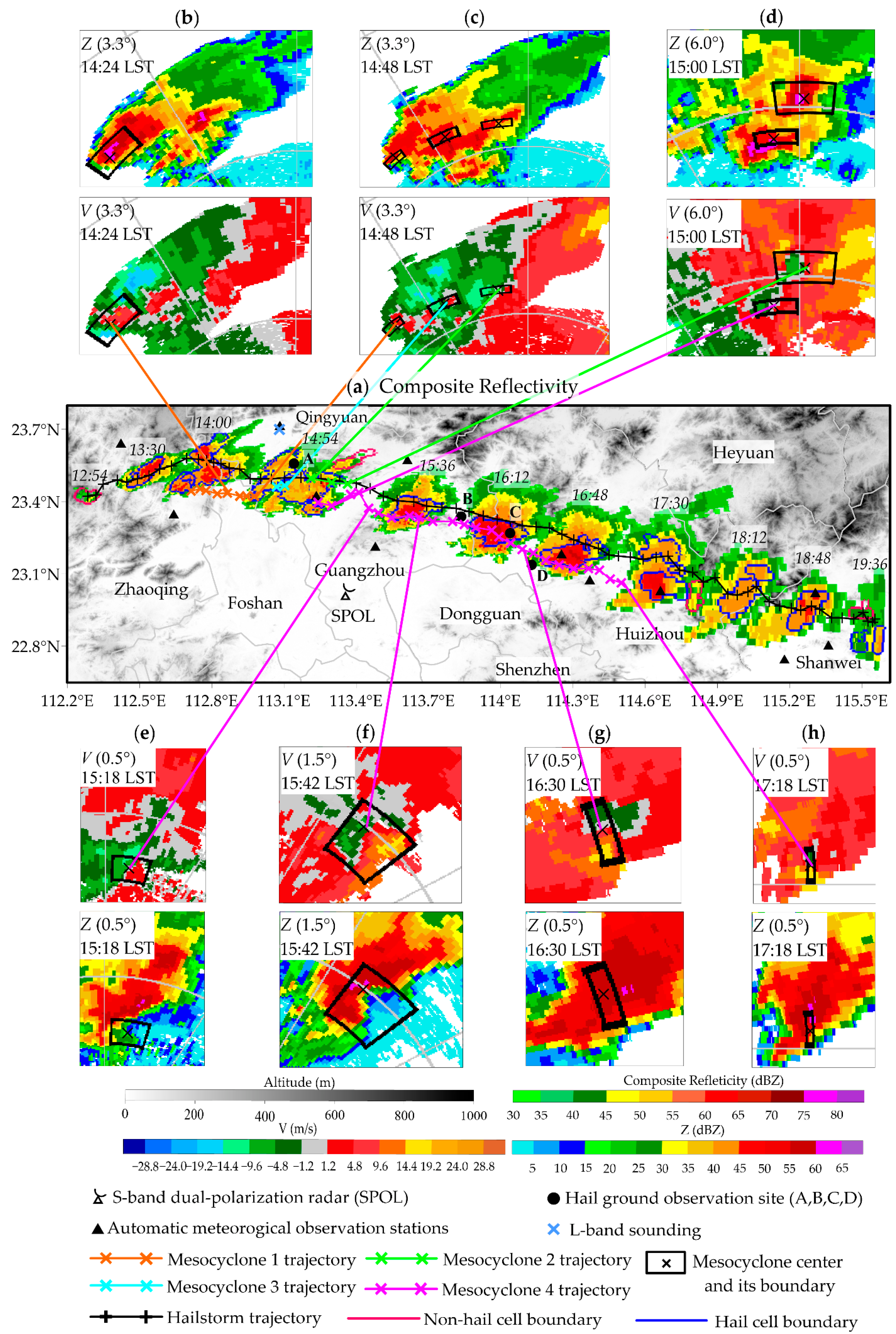
A15:08Qingyuan3.96.9
B16:02Guangzhou3.96.9
C16:00–16:30Huizhou3.96.9
D16:00–16:30Huizhou3.96.9
Table 4. Parameters for which the ICCE algorithm produces a time-series.
Convective Feature TypeParameterUnit
Convective system structural characteristicsCentroid position#
Height of center of masskm
Convective system topkm
Convective system basekm
Height of maximum reflectivitykm
Maximum reflectivitydBZ
Convective-system-based VILkg/m2
Maximum reflectivity on each plane *dBZ
Convective system microphysical characteristicsMaximum area of hail (or graupel)km2
Height of maximum hail (or graupel) areakm
Hail (or graupel) topkm
Hail (or graupel) basekm
Total area of hail (or graupel)km2
Total area of hail below the melting layerkm2
Hail (or graupel) area on each plane *km2
Storm cell (including non-hail cell and hail cell) microphysical and structural characteristics (within a convective system)Hail cell number1
Hail top (in the hail cell)km
Hail base (in the hail cell)km
Centroid position #
Storm cell topkm
Storm cell basekm
Storm-cell-based VILkg/m2
Maximum reflectivity of the storm celldBZ
Height of maximum reflectivity of the storm cellkm
Convective system mesocyclone characteristicsMesocyclone number1
Center position#
Mesocyclone total depthkm
Mesocyclone topkm
Mesocyclone basekm
Rotational velocity on each shear layer *m/s
Maximum rotational velocitym/s
Height of maximum rotational velocitykm
Shear on each shear layer *1/h
Maximum shear1/h
Height of maximum shearkm
Diameter on each shear layer *km
Maximum diameterkm
Height of maximum diameterkm
Height of each shear layer *km
Convective system tracking characteristicsConvective system ID1
Current convective system speedkm/h
Current convective system directiondeg
Forecast position#
The asterisk (*) represents the temporary storage parameters; the well number (#) denotes the location information in latitude and longitude; the parameter “Diameter” is the distance between maximum outbound velocity (Vmax) and maximum inbound velocity (Vmin).
Disclaimer/Publisher’s Note: The statements, opinions and data contained in all publications are solely those of the individual author(s) and contributor(s) and not of MDPI and/or the editor(s). MDPI and/or the editor(s) disclaim responsibility for any injury to people or property resulting from any ideas, methods, instructions or products referred to in the content.

