Article

Coupled Thorens and Soil Conservation Service Models for Soil Erosion Assessment in a Loess Plateau Watershed, China

1
State Key Laboratory of Earth Surface Processes and Resource Ecology, Faculty of Geographical Science, Beijing Normal University, Beijing 100875, China
2
Institute of Land Surface System and Sustainable Development, Faculty of Geographical Science, Beijing Normal University, Beijing 100875, China
3
School of Geography, University of Leeds, Leeds LS2 9JT, UK
4
School of Interdisciplinary Studies, University of Glasgow, Dumfries DG1 4ZL, UK
*
Author to whom correspondence should be addressed.
Remote Sens. 2023, 15(3), 803; https://doi.org/10.3390/rs15030803
Submission received: 8 December 2022 / Revised: 15 January 2023 / Accepted: 30 January 2023 / Published: 31 January 2023

Abstract

:
Assessing soil erosion in China’s severely eroded Loess Plateau is urgently needed but is usually limited by suitable erosion models and long-term field measurements. In this study, we coupled the Thorens and Soil Conservation Service (SCS) models to evaluate runoff and sediment yield during the 1980s and 2010s in the Xiaolihe watershed on the Loess Plateau. Results showed the proposed model framework had a satisfactory performance in modelling spatially distributed runoff and sediment yield. The Nash–Sutcliffe efficiency (NSE), percent bias (PBIAS) and the root mean square error-measured standard deviation ratio (RSR) were 0.93, 4.42% and 0.27 for monthly runoff; and 0.31, 62.31% and 0.82 for monthly sediment yield. The effects of land use changes on runoff and sediment yield were well captured by the SCS and Thorens models. The proposed modelling framework is distributed with a simple structure, requires relatively little data that can be obtained from public datasets, and can be used to predict runoff and sediment yield in other similar ungagged or poorly monitored watersheds. This work has important implications for runoff and erosion assessment in other arid and semi-arid regions, to derive runoff and erosion rates across large areas with scarce field measurements.

1. Introduction

Soil erosion is a global environmental threat to sustainable development [1,2,3,4]. The Yellow River in China is well known for its substantial sediment yield that accounts for approximately 6% of the total sediment loads from all rivers worldwide [5,6]. The Loess Plateau of China has a sediment yield that accounts for 88.2% of the total sediment load of the Yellow River [7,8,9]. Approximately 91,200 km2 area of the Loess Plateau has an erosion rate of more than 8000 t km−2 yr−1 (maximum erosion rate as 15,000 t km−2 yr−1), making the Loess Plateau the most severely eroded worldwide [10,11]. The severe soil erosion is mainly driven by a highly erodible loess with low cohesion, especially when there are wet, short-duration and high-intensity rainstorms, steep sloping topographic features, low vegetable cover and high-intensity cultivation [12,13,14]. The large amounts of sediment eroded and transported downstream lead to a wide range of problems, including land degradation, reduced food productivity, reservoir sedimentation, and water pollution. [8,12,15,16].
Soil erosion is difficult to quantify, particularly on a larger scale, as field measurements are usually conducted at limited temporal and spatial scales due to financial and time constraints [2,17]. Soil erosion models can provide a quantitative method to estimate erosion rates, and they have been widely used in the Loess Plateau of China [18,19]. In models, erosion is calculated as a function of driving forces (e.g., rainfall erosivity, runoff rate and gradient) and resistance to erosion (e.g., soil properties and vegetation cover) [20]. There are two general types of soil erosion models: empirical and process-based models [18,21]. Empirical models are normally based on the assumption that a linked system of interrill and channel elements can adequately represent the area of erosion, including the Universal Soil Loss Equation (USLE) and the revised version of the USLE (RUSLE) [15,22,23,24,25]. In contrast, process-based models tend to be adapted to the catchment scale, such as the Limburg Soil Erosion Model (LISEM) [26], and the Soil and Water Assessment Tool (SWAT) [7,27]. Most empirical models are generally built upon field plot measurements and might need to be calibrated for specific environments [18]. Hence, the application is limited, as the suitability and performance depend largely on the local circumstances. In contrast, the distributed models can capture key physical processes in runoff and erosion at the watershed scale. They can simulate spatial erosion patterns within a catchment [28]. However, the data required for distributed models might be tremendous, and a scarcity of high spatial and temporal scale resolution data in most watersheds has hampered their applications.
Due to the complicated landform and the relative lack of field measurements on the Loess Plateau, a simple and distributed model may be a better choice. In many cases, simpler lumped models perform similarly to distributed erosion models [29]. It is feasible to estimate soil erosion and its spatial distribution for large areas using satellite observations, Geographic Information system (GIS) technologies and low-data-demand models at a reasonable cost and accuracy without the need for time-consuming and expensive field surveys [30]. The conceptual erosion model developed by Thornes [31,32] provides such an option. The model has a simple structure including three components that depict key drivers of erosion: hydrology, sediment transport and vegetation cover. The Thornes soil erosion model has the following advantages: (i) the model includes four main components that affect soil erosion, and the model structure is simple, and (ii) the parameters are physical-process based and data are easy to acquire. This modelling approach has been used in humid and semi-arid environments [17,33,34,35,36,37]. For example, Saavedra [34] compared the Thornes model and four other conceptual models for modelling erosion in the Bolivian Andes with three climatic regions: dry, temperate humid, and tropical rainfall. Symeonakis, Calvo-Cases and Arnau-Rosalen [36] used the Thornes model to predict erosion rates for two catchments in southeastern Mediterranean Spain. The distributed Thornes model is able to predict potential erosion rates at different time scales (daily, monthly and yearly) at low input data requirements [17]. The Thornes erosion model is able to capture the major controlling factors in soil erosion (e.g., soil erodibility, surface runoff, slope steepness and vegetation cover) and the conditions prevailing in the loessial hilly gullied region [18]. It is hypothesized that the Thornes erosion model can estimate erosion rates and spatial distribution for large loess hilly gullied areas with low demand for data and at a reasonable cost and accuracy. However, no previous studies have been conducted and it is still unknown whether this erosion model can be used in typical agricultural watershed on the Loess Plateau.
Since the 1950s, a series of ecological conservation and restoration projects have been implemented to reduce water and soil losses by planting trees and grass on the Loess Plateau [12]. These restoration activities increased vegetation cover, altered land use patterns and led to changes in runoff and sediment yield [8,16,38]. Time series analysis and physically based modelling are two major methods to assess the effects of climate variation and land use change on catchment runoff and sediment yield. For example, Hessel, et al. [39], based on the simulated results of the LISEM, found that implementation of slope-steepness-based conservation strategies in the Danangou catchment would decrease runoff by 40–50% and soil erosion by 50–60%. Li, Liu, Zhang and Zheng [27] used the SWAT model and found that land use change in the Heihe catchment on the Loess Plateau decreased runoff by 9.6%. The combined effects of rainfall and land use drive runoff and soil loss changes. However, there are still different opinions on the degree of runoff and sediment change and the influence of various factors on the change. It is important to address this problem as regional scale assessment provides important information for local economic and social development and environmental protection.
This study coupled the time series analysis and distributed-based modelling method and coupled the Thorens and Soil Conservation Service models for soil erosion assessment in a typical agricultural watershed (Xiaolihe) in the Loess Plateau. The objectives of this study were to (i) evaluate the performance of the coupled Thornes and SCS models in predicting runoff and soil erosion, and (ii) to examine the effects of changes in land use on the runoff and sediment yield using time series analysis based on comparisons between the 1980s (from 1978 to1982) and 2010s (from 2006 to 2010). These results will provide decision makers with useful information to control soil erosion and implement appropriate land-management measures.

2. Materials and Methods

2.1. Study Area

The loessial hilly gullied region in the Loess Plateau of China has an area of 236,000 km2 (53% of the Loess Plateau), and acts as the main source of sediment for the Yellow River [40]. It has been widely reported that suspended sediment concentration in this region is greater than 1000 kg m−2 [26]. The Xiaolihe watershed, located in the loessial hilly gullied region, is among the most severely eroded areas in the Loess Plateau (Figure 1a). It has a reach of 63.7 km in length and a drainage area of 807 km2. The watershed is highly dissected by dense channel networks, with a drainage density (length of streams per unit area) ranging 4–8 km km−2 and an incision depth of 50–200 m. The climate is semi-arid with a mean annual precipitation of 397 mm [41], more than 70% of which occurs in the summer months (from July to September) as rainstorms. The slope can be as high as 70°. The loess soil layer is approximately 100 m thick with silt-rich (60%) soil texture. More than half of the Xiaolihe watershed is covered by cropland (Table 1), mainly distributed on the hilltops [26]. The most important crops are potatoes, millet, soybean, and maize [26]. Soil conservation practices began in the 1950s and have significantly enhanced since 1980 when the Chinese government implemented a series of ecological conservation and restoration, including planting vegetation (trees, bushes and grasses), improving grasslands, building terraced fields and warping dams. These measures (e.g., the Grain for the Green Project) have greatly changed the underlying surface, resulting in a decrease in farmland and increases in forest and grassland [27].

2.2. Model Descriptions

Soil erosion was estimated with the coupled Thornes model and the SCS-CN method. There are two major assumptions for the Thornes model: (i) daily precipitation can be approximately distributed as an exponential frequency within a certain period; (ii) the soil water-storage capacity is affected by the initial moisture content of the soil. In the Thornes model, the potential soil erosion of a computation unit is estimated as [17]:
E = kQ2s1.67e−0.07ci
where E (mm) is the erosion rate, k is the soil erodibility factor, Q (mm) is the overland flow, s (m m−1) is the slope gradient, and ci (%) is the fraction of vegetation cover. In this study, the sediment delivery ration was assumed as 1.0, since at the event or intra-annual and annual timescales hyper-concentrated flows are well developed and have strong sediment-carrying capacity in the Loess Plateau [42,43].
Overland flow Q is a key parameter of the above erosion model from Formula (1) that can be deduced from the SCS method [44,45]. The SCS method is mainly based on the water balance equation and two hypotheses which can be expressed as:
P = Ia + F + Q
and the two hypotheses are as follows:
Q/(PIa) = F/S
Ia = λS
where Q (mm) is direct runoff, P (mm) is precipitation, Ia (mm) refers to the initial abstraction, F (mm) indicates the cumulative infiltration excluding Ia, S (mm) is the potential maximum retention, and λ is the initial abstraction ratio.
Combining Equations (2)–(4) gives an expression for Q:
Q = (PλS)2/[(P + (1 − λ)S)]
The initial abstraction ratio λ in the standard CN method is 0.2, and Equation (5) can be written as:
Q = (P − 0.2S)2/(P + 0.8S) P > 0.2S
Q = 0        P <= 0.2S
The value of S is obtained from:
S = 254(100/CN − 1)
where CN is a comprehensive parameter (with values range from 0 to 100) that indicates the runoff potential governed by soil antecedent moisture condition (AMC), slope gradient, cover type, soil property and land use.
The AMC represents soil moisture prior to a runoff event according to the 5-day antecedent rainfall depth in growing or dormant seasons [45], including dry (AMC I), moderate (AMC II), and wet (AMC III) conditions. The corresponding CN under these three conditions is denoted CN1, CN2 and CN3, respectively. The SCS model provides the reference value of CN2 of different land use types and land surface infiltration categories in the handbook table (USDA–SCS, 1972). Considering the existing steep slope terrain of the Loess Plateau of China, the CN2 was modified as CN2x by the slope gradient s (m m−1) [45]:
CN2x = CN2(322.79 + 15.63s)/(s + 323.52)
The CN2x values for different land uses were estimated based on published literature [44]. The relationships between CN2 value and CN1 and CN3 are given in Equations (10) and 11 [46]. The estimated CN values are given in Table 2.
CN1 = CN2/(2.281 − 0.01281CN2)
CN3 = CN2/(0.427 + 0.00573CN2)
The Nash–Sutcliffe model efficiency (NSE), percent bias (PBIAS) and the root mean square error-measured standard deviation ratio (RSR) were chosen to assess the predictive performance of the Thornes model [47]. The expressions are as follows:
N S E = 1 i = 1 n ( Q obs Q sim ) 2 / i = 1 n ( Q obs m e a n ( Q obs ) ) 2  
P B I A S = i = 1 n ( Q obs Q sim ) / i = 1 n Q obs  
R S R = i = 1 n ( Q obs Q sim ) 2 / i = 1 n ( Q obs m e a n ( Q sim ) ) 2
where Qobs is the measured runoff and sediment yields, Qsim is the simulated runoff and sediment yields, and n is the total number of data records. The NSE ranges between −∞ and 1, with an optimal value of 1.0. When NSE values range between 0 and 1, the model performance is regarded as acceptable; whereas negative NSE values indicate an unacceptable performance of the model. The optimal value of PBIAS is 0. Low-magnitude values illustrate accurate model simulation; positive or negative values show underestimation or overestimation bias, respectively. PSR values range from 0 to a large positive value, and the optimal RSR value is 0.

2.3. Data Collection and Model Input

2.3.1. Hydrology

Hydrological data for the Xiaolihe watershed are very scarce, and long-term, continuous runoff and sediment yield data were available only for eight existing and discontinued basin gauging stations (Figure 1a). The Yellow River Water Conservancy Commission (YRWCC) provided the aggregate monthly rainfall data (seven precipitation stations) and the average monthly streamflow and sediment (one hydrometric station) data.

2.3.2. Topography

The digital elevation model (DEM) and slope gradient (Figure 1b) were derived from the 30 m global digital elevation model (GDEM) dataset that is a product of the Advanced Spaceborne Thermal Emission and Reflection Radiometer (ASTER). The raw grid type of the DEM data (in the WGS84 coordinates system) was preprocessed in ArcInfo ArcGIS to fill sinks. Based on an automatic procedure with ArcSWAT 2.3.4, 25 hydrologically connected sub-basins were segmented, with each area less than 100 km2.

2.3.3. Soil Properties

Basic soil physical and chemical properties were extracted from China’s National Second Soil Survey Data and Soil Types [48]. On the Loess Plateau, the soils are cohesive due to low levels of organic matter and high levels of silt and clay [49]. The proportion of the soil types characterized by cultivated loessial and alluvial soil was relatively high. According to Stone and Hilborn [50], these soil types can be classified as silt loam and sandy loam in soil texture, with the soil erodibility k factor being 0.3 and 0.18, respectively.

2.3.4. Land Use

We collected time series of satellite imagery in the summer months (i.e., from June to August) when most of the study area’s soil erosion and sediment transport is caused by summer rainstorms. A man–machine interaction method was used to extract the land use information in the 1980s and 2010s from two phrases of Landsat TM imagery (Figure 1c,d). The land use data included six Level 1 and 31 Level 2 categories. The land use data interpretation accuracy was assessed with field validations, historical records and maps, and interviewing local elder residents [51]. The accuracy for the 1980s and 2010s land use data interpretation was 73.7% and 89.5%, respectively.

2.3.5. Vegetation Cover

Vegetation cover was estimated by its linear relationship with the normalized difference vegetation index (NDVI) [52].
Ci = 8.79815 + 93.07466NDVIi
where Ci is the vegetation cover for a cell during period i (%), and NDVIi is the normalized difference vegetation index during period i. This study used the 250 m spatial resolution MODIS NDVI and quality assurance as 16-day products (ISDSP, 2010b).
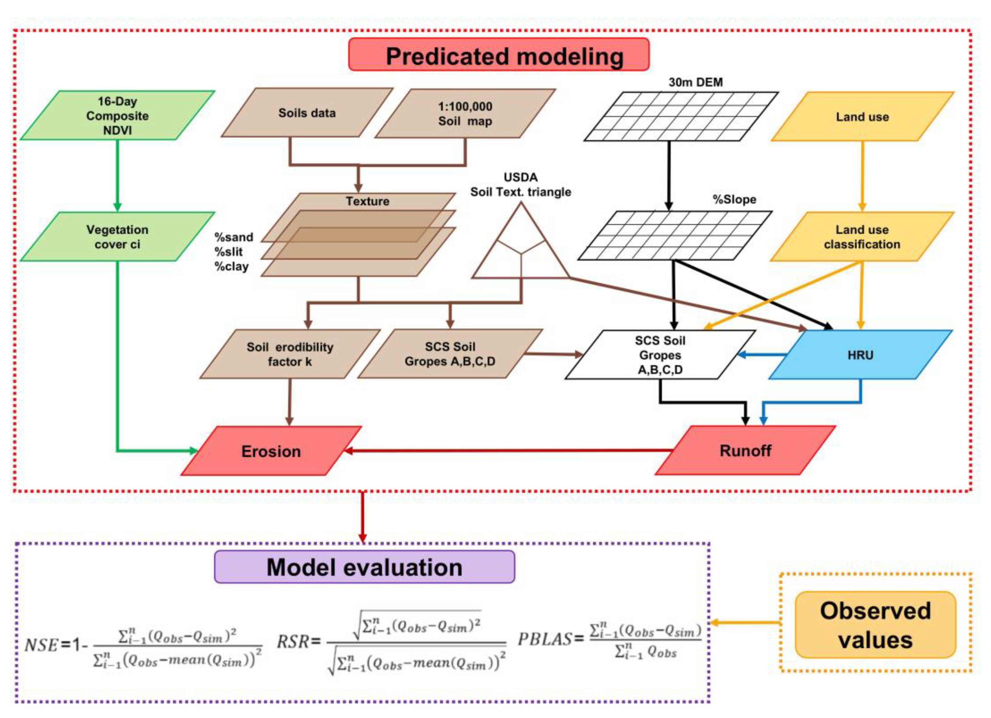
The coupled Thornes erosion model (Equation (1)) and the runoff sub-model (Equations (6) and (7)) was applied at the hydrological response unit (HRU) spatial scale and monthly time step for calculating potential runoff (m3 s−1) and erosion rates (mm month−1) for the Xiaolihe watershed. The HRU was employed as the minimum computation unit, reflecting a homogeneous hydrological process dynamics from combinations and distributions of physiographic basin properties, including land use, soil type and slope gradient [27,53,54]. Two periods, the 1980s (from 1978 to 1982) and 2010s (from 2006 to 2010), were selected to represent land use with significant changes. Figure 2 shows the model framework and its schematic representation of data flow and processing. All layers were resampled to HRUs and then calculated using geospatial modelling procedures in ArcInfo ArcGIS.
To examine how land use or precipitation changes affect runoff and sediment yield, pairwise comparisons were conducted between two years with similar annual precipitation or land use, respectively. The observed and simulated runoff and sediment datasets were tested for normality using the Anderson–Darling test. Then, either the Student t-test or the Mann–Whitney U-test was applied to test for a significant difference in the means or the medians of the runoff or sediment between two paired treatments. Parametric tests were used when both datasets being considered were normally distributed, and non-parametric tests were used for datasets when at least one was not normally distributed. Test results were considered significant at p < 0.05.

3. Results

3.1. Modelling Monthly Runoff

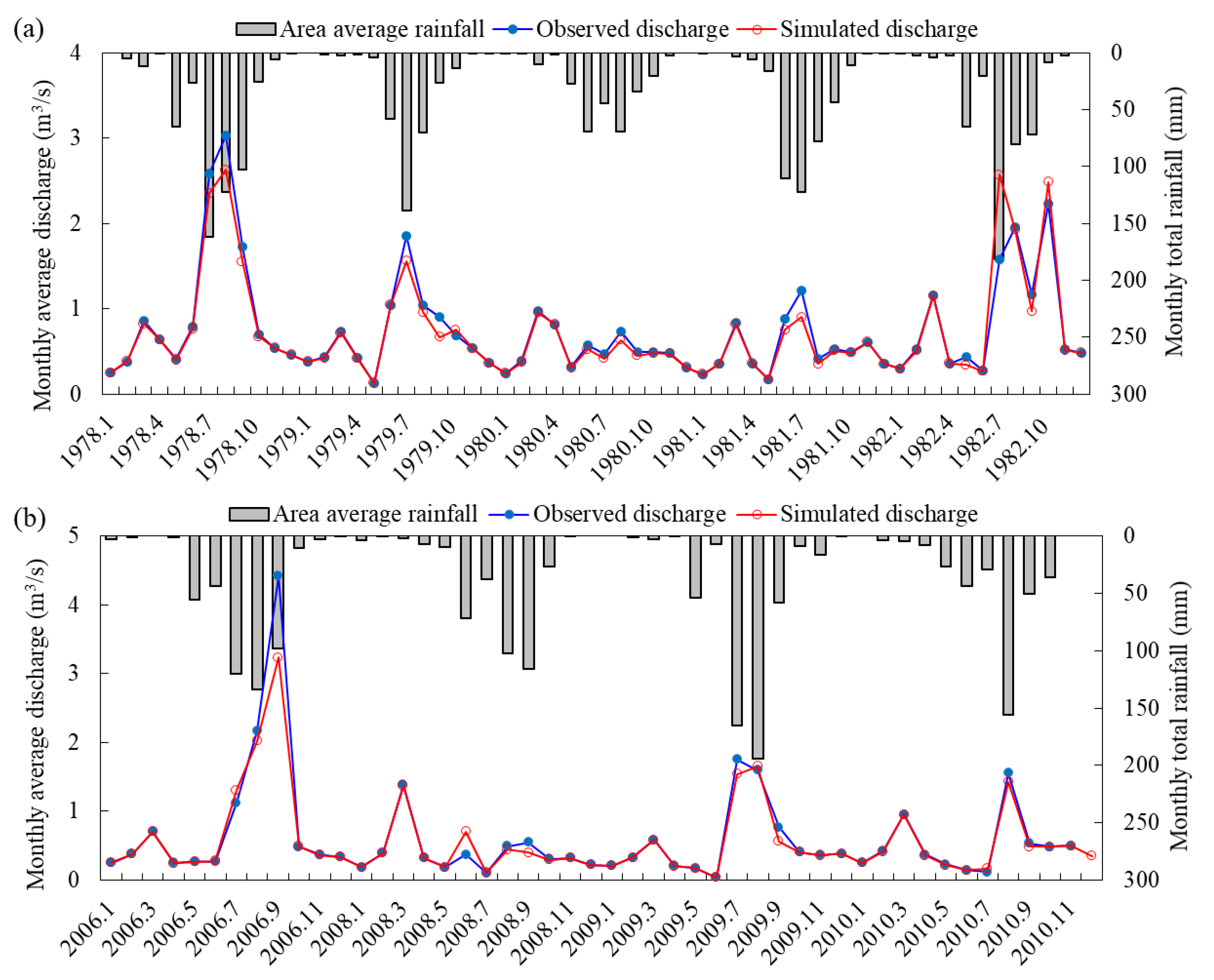
The base flow was separated based on the graphical approach from the streamflow time series, and the proportion of base flow in streamflow was 49%. The SCS surface runoff model (Equation (5)) was calibrated well to simulate the measured monthly average runoff discharge (Figure 3). Specifically, between 1978 and 1982, the observed and simulated monthly average runoff discharges were 0.744 and 0.720 m3/s, respectively, and the NSE, PBIAS and RSR were 0.92, 3.30% and 0.28, respectively. During 2006–2010, the observed and simulated monthly average runoff discharges were 0.597 and 0.564 m3/s, respectively. Accordingly, the NSE, PBIAS and RSR were 0.93, 5.54% and 0.26, respectively. Model simulation is generally considered satisfactory if the NSE > 0.50, PBIAS ± 55%, and the RSR < 0.70 [47]. The SCS performance for monthly discharges was “very good” during 1978–1982 and 2006–2010, and the 2010s had a better performance than the 1980s. These results show that the SCS model can efficiently describe changes in monthly discharges at the Xiaolihe watershed. The temporal patterns of predicted monthly discharge rates had no significant difference (p = 0.742) with the observed discharge rates at the watershed outlet gauging station, and the correlation between the two was strong (r2 = 0.934). These results suggest that the SCS model can be applied to estimate monthly runoff discharges in other ungagged basins. However, the SCS model underestimated the monthly discharge for the August and September rainy months (Figure 4). The high discharge events were not well matched with the corresponding simulations, which tended to be lower during most summers with concentrated rainfall.

3.2. Modelling Monthly Sediment

The Thornes model could well capture the average monthly sediment delivery trend, showing a good contingency between the modelling and measured soil erosion rates (Figure 5). Between 1978 and 1982, the observed and simulated monthly average sediment discharges were 32.41 and 31.36 kg/m3, respectively. The NSE, PBIAS and the RSR were 0.94, 3.24% and 0.25, respectively. From 2006 to 2010, the observed and simulated values were 68.95 and 83.30 kg/m3, respectively. The NSE, PBIAS and the RSR were 0.85, 20.82% and 0.39, respectively. The sediment delivery during the rainy seasons (from June to September) ranged from 51.737 kg/s to 229.811 kg/s, substantially higher than the other months (0.000 kg/s–7.294 kg/s; average, 1.347 kg/s) (Figure 6) with little or no rainfall. Results showed that the four rainy months contributed to 98% of the total annual soil loss. There was a strong correlation (r2 = 0.878) between the predicted and observed monthly sediment yield. The temporal patterns of the two data series had no significant difference (p = 0.791), suggesting that the predicted model can be applied to estimate erosion rates in ungauged basins. Overall, the Thornes erosion model produced sound sediment yield predictions. However, the predictions were less satisfactory from June to September, in which the simulated sediment yields were generally smaller than the observed values.

3.3. Effects of Land Use Change on Runoff and Sediment

The dominant land uses in the Xiaolihe watershed were farmlands and grassland (Table 1), which accounted for about 95% of the entire area (97.0% and 94.2% for the 1980s and 2010s, respectively). In the 1980s, plain cropland covered most of the watershed (55.33% of the whole region, 449.87 km2), followed by grassland with low and moderate coverage, with an area of 257.65 km2 (31.69%) and 65.71 km2 (8.08%), respectively. In the 2010s, plain cropland and moderate-coverage grassland were the dominant land uses, accounting for 92.65% of the entire watershed area. There were two main trends of land use changes during 1980–2010: the increase in moderate-coverage grassland and the decrease in low-coverage grassland and croplands. Compared with the 1980s, moderate-coverage grassland, open forest land, shrubland, and forest in 2010s increased by 265.17, 10.61, 6.78, and 4.08 km2, respectively, while low-coverage grassland, plain and montanic cropland decreased by 254.53, 27.32, and 6.51 km2, respectively; high-coverage grassland, water area and construction land showed little change compared to their baselines of 1980s.
Table 3 gives the main land use conversions. The main land use conversions showed that 35.68% of the entire watershed, or 290.08 km2 underwent type conversions. There were seven types of changes whose areas were more than 1 km2. The changes fell into two groups: one was the conversion of low-coverage grassland to moderate-coverage grassland (254.53 km2), and the other was the conversion of farmland to other land uses (33.84 km2).
To examine the effects of land use change on runoff and sediment yield, three hypothetical scenarios with similar annual precipitation (p > 0.05) but different land uses were compared (Table 4). Compared to the 1980s, both the simulated and observed discharges generally decreased, representing the effects of land use change. For example, the observed and simulated average runoff rate in 2009 decreased by 0.46 m3/s (−45%) and 0.42 m3/s (−44%) than 1978, respectively. It should be noted that the simulated runoff reductions caused by land use change were slightly lower than the observed reductions. For all three studied scenarios, the land use change over the whole watershed increased sediment yiled but the differences between the two studied years were insignificant at p = 0.05.

3.4. The Combined Effects of Rainfall and Land Use Change on the Temporal and Spatial Patterns of Erosion Rates

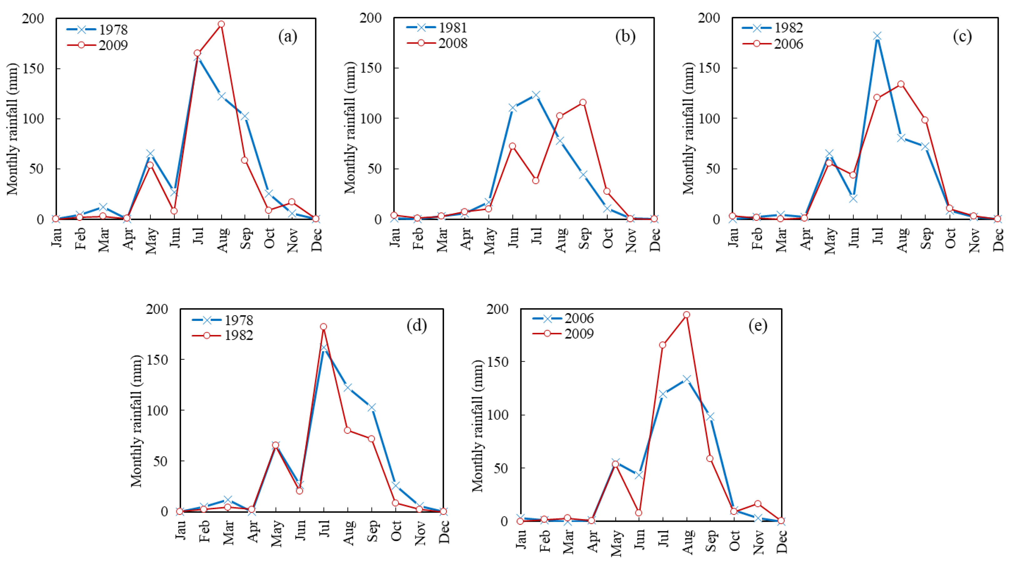
The observed and simulated sediment yield increased in the 2010s compared to their baselines of the 1980s (Table 4). For a closer comparison of the temporal and spatial variations in soil erosion among different conditions, monthly potential erosion rates were summed to obtain annual erosion rates and were grouped into five classes [55] (Table 5). The comparisons of the monthly rainfall distribution of the five groups are illustrated in Figure 7. Pairwise comparisons were conducted between two years, and five hydrological year groups (Group 1–5): Group 1–3 includes Group 1 (1978 vs. 2009), Group 2 (1981 vs. 2008), and Group 3 (1982 vs. 2006), indicating that each group has two years with similar annual precipitation but different land use; Group 4–5 includes Group 4 (1978 vs. 1982), and Group 5 (2006 vs. 2009), showing that each group has two years with similar land use but different annual precipitation. By doing this, the effects of changes in land use or precipitation on the temporal and spatial patterns of sediment yield were examined.
Pairwise comparisons for Groups 1–3 showed that the areas with very high (5.0−10.0 mm/year) and extreme (>10.0 mm/year) erosion risk increased from the 1980s to the 2010s (Table 5). For Group 1 (1978 vs. 2009): In 1978, 90.23% of the basin experienced slight (0–0.2 mm/year) to moderate erosion (0.2–1.0 mm/year). The high (1.0–5.0 mm/year) and extreme (>10 mm/year) erosion intensities were only 1.54% and 8.23%, respectively. In contrast, in 2009, the percentage of areas with an extreme erosion rate increased from 8.23% to 14.33% (Table 5). For Group 2 (1981 vs. 2008): compared to 1981, the sediment yields in 2008 increased by 0.082 × 10⁶t up to 0.476 × 10⁶t (Table 4), although land use tends to be better rehabilitation for soil conservation. Modelling results illustrated that 91.61% of the watershed appeared to be under the condition of slight erosion (0–0.2 mm/year), and only 6.91% of the total area experienced a very high (5.0–10.0 mm/year) to extremely high intensity of erosion (>10.0 mm/year) in 1981. However, remarkable changes took place in 2008. The slight erosion area declined from 91.61% to 52.92%. Meanwhile, the area with extreme soil intensity increased from 3.77% to 9.59% (Table 5). For Group 3 (1982 vs. 2006): the ratio of extreme soil intensity doubled to 16.22% in 2006 compared with 8.23% in 1982.
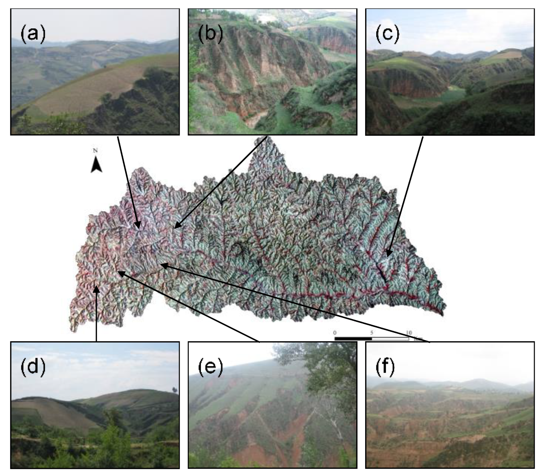
The quantity of soil erosion in the northwestern and middle parts of the Xiaolihe watershed was reduced due to a large amount of grassland with low cover undergoing conversion to grassland with moderate cover and the conversion of agricultural terraces to grassland or forest. According to the spatial distribution of predicted annual erosion rates, the hotspots showed a considerable increase in erosion potential. These hotspots were characterized by steep sloping topographic features and low vegetation coverage but high-intensity cultivation (Figure 8). For example, areas within ellipse within category “A” accounted for 5.06% of the severe erosion intensity (>10.0 mm/year), more than that of 1978. The uneven distribution of annual rainfall also caused temporal changes in erosion rates. The temporal pattern showed that the occurrence of rainstorms in the 2010s tended to lag than that of the 1980s. For instance, the precipitation in 1981 was concentrated in June and July when the vegetation cover was higher. In 2008, the recorded rainfall for two months (August and September) accounted for 56.05% of the whole year (Figure 7b). It reached a maximum in September when the mean precipitation was the highest (120 mm), and vegetation cover was slightly decreased because of farming or grazing in the summer months. In addition, the 2010s had more frequent short-duration and high-intensity rainstorms which are vital in increasing soil erosion. In this area, the annual sediment yield can mainly result from one or two heavy storms. For example, for the abovementioned hotspot A, in August 2009, the precipitation of the recorded maximum storm events was 105 mm, leading to high erosion rates caused by severe hilly headward erosion. Another example is that on 20 September 2006, the Xiaolihe watershed experienced among the heaviest rains on record, with a maximum precipitation of 79 mm within 2 h. Moreover, the spatial and temporal rainfall distribution in 2006 was significantly uneven (Figure 7c). Therefore, the most remarkable variation during these two years was that the percentage of areas with very high and extreme erosion potential increased by 30.06% and 7.99%, respectively (Table 5), resulting in the total annual sediment discharge increasing by 2.517 × 10⁶ t.
For Group 4 (1978 vs. 1982), there was no significant change in the annual distribution of rainfall, and the precipitation in 1978 was 89 mm more than that in 1982. However, the sediment discharge observed showed the inverse trend in 1978 and 1982, with values of 1.831 × 10⁶ and 3.153 × 10⁶ (Table 4), respectively. This may be because the area with high erosion increased slightly from 12 to 28 km2. The rainfall in 1978 was relatively evenly distributed in July, August and September, while the precipitation in 1982 was concentrated at the end of July and the beginning of August, characterized by several heavy storms that caused over 90% sediment yield throughout the year. Similarly, in Group 5, the rainfall in 2006 and 2009 was concentrated in the summer months (July, August and September). The precipitation in these two years was 471 and 510 mm, but more heavy storms occurred in 2006 than in 2009. Thus, the sediment discharge in 2006 nearly doubled that in 2009. Moreover, at the end of the wet season, such as September 2006, the largest amount of rainfall (79 mm) caused the highest amounts of sediment discharge (39,700 kg/s) for the year.

4. Discussion

4.1. Application of the Proposed Modelling Framework

Large-scale quantification of soil erosion is usually difficult due to the labor, costs and time involved [2]. Based on the coupled Thorens and Soil Conservation Service (SCS) models, we provided a distributed modelling framework with a simple structure and low dataset requirements for assessing runoff and sediment and the effects of land use changes in the Loess Plateau. The satisfactory modelling accuracy demonstrated that the method employed in our study worked well. This work has important implications for runoff and erosion assessment in other arid and semi-arid regions to derive runoff and erosion rates across large areas with scarce field measurements.
The significant increases in moderate-coverage grassland and changes of farmland to others were mainly caused by the implementation of “the grain-for-green project” initiated in 1999 [6,11,12]. Different land use patterns have varied soil physicochemical properties and thus should have different effects on the rainfall–runoff and the runoff–sediment relationships [39,56,57]. The effects of land use changes on runoff and sediment yield were well captured by the SCS and Thorens models.
However, it should be noted that the SCS and Thorens models performed better in modelling runoff and sediment than those for the rainy seasons. The monthly discharge was underestimated for the August and September rainy months (Figure 4). The high discharge events were not well matched with the corresponding simulations, which tended to be too low during most summers with concentrated rainfall. The slope-modified CN method used in this study was found to increase runoff prediction for steep slopes prevalent in the Loess Plateau [45], but might still underestimate large runoff events. Li, Liu, Zhang and Zheng [27] applied the SCS model to an agricultural watershed in this region; the monthly runoff performance was not as robust as that for annual runoff. These findings corroborated the simulated runoff data in the Xiaolihe watershed. The main reason for the above difference is that mean daily rainfall depths, instead of the duration and intensity of precipitation typical in the studied watershed, were put into the SCS model [58,59]. The rainfall in June and July accounted for 90% of the total months’ rainfall. Thus, the SCS model tended to underestimate overland runoff generated from this form of rainstorm [60]. In addition, SCS-CN methods ignore several storms occurring during a single day, which might lead to the underestimation of runoff. The slope-adjusted CN equation increased the accuracy of runoff prediction in the sloping regions of the Loess Plateau of China [44,45], further improvements or adjustments are still needed to consider local conditions and incorporate characteristics of extreme precipitation and runoff events [54,61,62].
The Thorens approach showed satisfactory validation, suggesting a reliable prediction of the spatial patterns of erosion rates. However, the quantitative prediction should be interpreted with caution. The sub-basins with steep slopes and a substantial proportion of heavy rainstorms tended to have high erosion rates. These subregions in the Xiaolihe watershed are in line with severe land degradation, as reported by Zheng, Qin, Sun, Qi and Cai [40] based on measurements of suspended sediment yields. However, even though the rainstorm characteristics were not built into the model for predicting erosion, good results were produced by the modelling framework.

4.2. Advantages and Limitations

The proposed spatially distributed modelling framework gives satisfactory runoff and sediment yield predictions in the large, data-sparse Xiaolihe watershed. The coupled Thornes erosion model and SCS runoff model are physical-based, suitable for the studied arid and semi-arid environments, available for quick large-scale assessment through implementation in a GIS, and have low data requirements. These advantages suggest that the modelling framework presented in this study can estimate runoff and sediment yield in other ungagged drainage watersheds with similar conditions (e.g., hydrometeorology, topography and land use). However, the SCS model underestimated runoff in wet seasons with concentrated rainfall. The Thornes model underestimated sediment discharge from June to September, which may be mainly attributed to the type of rainfall and the frequency of intense rainfall. The disparity between the observed and simulated data indicates that the modification of Thornes components is needed to take rainfall intensity and its duration into account to increase the accuracy of peak runoff and sediment yield predictions in storms.
The application of a spatially distributed erosion model is usually constrained by model validation [28]. In this study, the model parameters were determined without field calibration due to a lack of field measurements. The model was validated by comparing the measured and predicted sediment yield at the catchment outlet, which is usually applied on the Loess Plateau [63]. Satisfactory and reliable modelling results were produced for the ungauged sub-basins within the Xiaolihe watershed. However, the Thornes model gives some abnormally high erosion rates. Similar anomalies were also found by Ali and De Boer [17] in the mountainous upper Indus River basin and by Symeonakis, Calvo-Cases and Arnau-Rosalen [36] in the Xaló River basin in southeastern Spain. This could be caused by the exponential nature of the empirical relationship, and possible quality problems in some spatial datasets [17]. Although the Thornes model was found to be a useful tool for assessing soil erosion and the effects of land use and precipitation change, further model improvement is needed to increase the prediction accuracy by including rainfall characteristics such as rainfall intensity and frequency of intense rainfall.

5. Conclusions

This study presented a modelling framework for estimating runoff and soil erosion in the Xiaolihe watershed of the Chinese Loess Plateau. By coupling the SCS and Thornes models for surface runoff and soil loss prediction, the simulated runoff and sediment discharges were compared with the daily observed datasets, including 108 rainstorm events during 1978–1982 and 2006–2010. The coupled Thorens and SCS models were a powerful tool to simulate runoff and sediment yield. The proposed spatially distributed modelling framework produced satisfactory runoff and sediment yield predictions in the large, data-sparse Xiaolihe watershed. It can be used for other ungagged drainage basins with similar situations. The modelling framework well captured the effects of land use changes on runoff and sediment yield. However, further improvements or adjustments are needed to increase prediction accuracy by incorporating extreme rainfall characteristics and runoff events. The results are beneficial for assessing land degradation and improving the ecological environment in the future.

Author Contributions

Conceptualization, C.L. and S.W.; methodology, C.L. and T.L.; software, C.L. and T.L.; validation, C.L.; writing—original draft preparation, C.L. and T.L.; writing—review and editing, C.L., T.L., S.W. and J.X.; visualization, C.L. and T.L.; supervision, S.W.; funding acquisition, C.L. and S.W. All authors have read and agreed to the published version of the manuscript.

Funding

This research was jointly funded by the National Natural Science Foundation of China Project (grant U2243601, 42007052), and the Fundamental Research Funds for the Central Universities.

Data Availability Statement

Not applicable.

Conflicts of Interest

The authors declare no conflict of interest.

References

  1. Li, C.; Fu, B.; Wang, S.; Stringer, L.C.; Wang, Y.; Li, Z.; Liu, Y.; Zhou, W. Drivers and impacts of changes in China’s drylands. Nat. Rev. Earth Environ. 2021, 2, 858–873. [Google Scholar] [CrossRef]
  2. Li, C.; Holden, J.; Grayson, R.; Li, P. Erosion in peatlands: Recent research progress and future directions. Earth-Sci. Rev. 2018, 185, 870–886. [Google Scholar] [CrossRef]
  3. Borrelli, P.; Robinson, D.A.; Fleischer, L.R.; Lugato, E.; Ballabio, C.; Alewell, C.; Meusburger, K.; Modugno, S.; Schütt, B.; Ferro, V. An assessment of the global impact of 21st century land use change on soil erosion. Nat. Commun. 2017, 8, 2013. [Google Scholar] [CrossRef] [PubMed] [Green Version]
  4. Borrelli, P.; Robinson, D.A.; Panagos, P.; Lugato, E.; Yang, J.E.; Alewell, C.; Wuepper, D.; Montanarella, L.; Ballabio, C. Land use and climate change impacts on global soil erosion by water (2015–2070). Proc. Natl. Acad. Sci. USA 2020, 117, 21994–22001. [Google Scholar] [CrossRef]
  5. Miao, C.; Ni, J.; Borthwick, A.G. Recent changes of water discharge and sediment load in the Yellow River basin, China. Prog. Phys. Geogr. 2010, 34, 541–561. [Google Scholar] [CrossRef] [Green Version]
  6. Wang, S.; Fu, B.; Liang, W. Developing policy for the Yellow River sediment sustainable control. Natl. Sci. Rev. 2016, 3, 162–164. [Google Scholar] [CrossRef] [Green Version]
  7. Zuo, D.; Xu, Z.; Yao, W.; Jin, S.; Xiao, P.; Ran, D. Assessing the effects of changes in land use and climate on runoff and sediment yields from a watershed in the Loess Plateau of China. Sci. Total Environ. 2016, 544, 238–250. [Google Scholar] [CrossRef]
  8. Zhao, G.; Mu, X.; Wen, Z.; Wang, F.; Gao, P. Soil erosion, conservation, and eco-environment changes in the Loess Plateau of China. Land Degrad. Dev. 2013, 24, 499–510. [Google Scholar] [CrossRef]
  9. Gao, P.; Mu, X.-M.; Wang, F.; Li, R. Changes in streamflow and sediment discharge and the response to human activities in the middle reaches of the Yellow River. Hydrol. Earth Syst. Sci. 2011, 15, 1–10. [Google Scholar] [CrossRef] [Green Version]
  10. Shi, H.; Shao, M. Soil and water loss from the Loess Plateau in China. J. Arid Environ. 2000, 45, 9–20. [Google Scholar] [CrossRef]
  11. Chen, L.; Wei, W.; Fu, B.; Lü, Y. Soil and water conservation on the Loess Plateau in China: Review and perspective. Prog. Phys. Geogr. 2007, 31, 389–403. [Google Scholar] [CrossRef]
  12. Fu, B.; Wang, S.; Liu, Y.; Liu, J.; Liang, W.; Miao, C. Hydrogeomorphic ecosystem responses to natural and anthropogenic changes in the Loess Plateau of China. Annu. Rev. Earth Planet. Sci. 2017, 45, 223–243. [Google Scholar] [CrossRef]
  13. Wu, X.; Wei, Y.; Fu, B.; Wang, S.; Zhao, Y.; Moran, E.F. Evolution and effects of the social-ecological system over a millennium in China’s Loess Plateau. Sci. Adv. 2020, 6, eabc0276. [Google Scholar] [CrossRef] [PubMed]
  14. Hessel, R. Consequences of hyperconcentrated flow for process-based soil erosion modelling on the Chinese Loess Plateau. Earth Surf. Process. Landf. 2006, 31, 1100–1114. [Google Scholar] [CrossRef]
  15. Sun, W.; Shao, Q.; Liu, J.; Zhai, J. Assessing the effects of land use and topography on soil erosion on the Loess Plateau in China. Catena 2014, 121, 151–163. [Google Scholar] [CrossRef]
  16. Wang, S.; Fu, B.; Piao, S.; Lü, Y.; Ciais, P.; Feng, X.; Wang, Y. Reduced sediment transport in the Yellow River due to anthropogenic changes. Nat. Geosci. 2016, 9, 38–41. [Google Scholar] [CrossRef]
  17. Ali, K.F.; de Boer, D.H. Spatially distributed erosion and sediment yield modeling in the upper Indus River basin. Water Resour. Res. 2010, 46, W08504. [Google Scholar] [CrossRef]
  18. Li, P.; Mu, X.; Holden, J.; Wu, Y.; Irvine, B.; Wang, F.; Gao, P.; Zhao, G.; Sun, W. Comparison of soil erosion models used to study the Chinese Loess Plateau. Earth-Sci. Rev. 2017, 170, 17–30. [Google Scholar] [CrossRef] [Green Version]
  19. Wen, X.; Deng, X. Current soil erosion assessment in the Loess Plateau of China: A mini-review. J. Clean. Prod. 2020, 276, 123091. [Google Scholar] [CrossRef]
  20. Wu, B.; Wang, Z.; Zhang, Q.; Shen, N.; Liu, J. Modelling sheet erosion on steep slopes in the loess region of China. J. Hydrol. 2017, 553, 549–558. [Google Scholar] [CrossRef]
  21. Borrelli, P.; Alewell, C.; Alvarez, P.; Anache, J.A.A.; Baartman, J.; Ballabio, C.; Bezak, N.; Biddoccu, M.; Cerdà, A.; Chalise, D. Soil erosion modelling: A global review and statistical analysis. Sci. Total Environ. 2021, 780, 146494. [Google Scholar] [CrossRef] [PubMed]
  22. Fu, B.; Zhao, W.; Chen, L.; Zhang, Q.; Lü, Y.; Gulinck, H.; Poesen, J. Assessment of soil erosion at large watershed scale using RUSLE and GIS: A case study in the Loess Plateau of China. Land Degrad. Dev. 2005, 16, 73–85. [Google Scholar] [CrossRef]
  23. Jin, F.; Yang, W.; Fu, J.; Li, Z. Effects of vegetation and climate on the changes of soil erosion in the Loess Plateau of China. Sci. Total Environ. 2021, 773, 145514. [Google Scholar] [CrossRef] [PubMed]
  24. Fu, B.; Liu, Y.; Lü, Y.; He, C.; Zeng, Y.; Wu, B. Assessing the soil erosion control service of ecosystems change in the Loess Plateau of China. Ecol. Complex. 2011, 8, 284–293. [Google Scholar] [CrossRef]
  25. Li, P.; Chen, J.; Zhao, G.; Holden, J.; Liu, B.; Chan, F.K.S.; Hu, J.; Wu, P.; Mu, X. Determining the drivers and rates of soil erosion on the Loess Plateau since 1901. Sci. Total Environ. 2022, 823, 153674. [Google Scholar] [CrossRef]
  26. Hessel, R.; van Asch, T. Modelling gully erosion for a small catchment on the Chinese Loess Plateau. Catena 2003, 54, 131–146. [Google Scholar] [CrossRef]
  27. Li, Z.; Liu, W.-Z.; Zhang, X.-C.; Zheng, F.-L. Impacts of land use change and climate variability on hydrology in an agricultural catchment on the Loess Plateau of China. J. Hydrol. 2009, 377, 35–42. [Google Scholar] [CrossRef]
  28. Feng, X.; Wang, Y.; Chen, L.; Fu, B.; Bai, G. Modeling soil erosion and its response to land-use change in hilly catchments of the Chinese Loess Plateau. Geomorphology 2010, 118, 239–248. [Google Scholar] [CrossRef]
  29. Jetten, V.; Govers, G.; Hessel, R. Erosion models: Quality of spatial predictions. Hydrol. Process. 2003, 17, 887–900. [Google Scholar] [CrossRef]
  30. Nearing, M.; Romkens, M.; Norton, L.; Stott, D.; Rhoton, F.; Laflen, J.; Flanagan, D.; Alonso, C.; Binger, R.; Dabney, S. Measurements and models of soil loss rates. Science 2000, 290, 1300–1301. [Google Scholar] [CrossRef]
  31. Thornes, J. The ecology of erosion. Geography 1985, 70, 222–235. [Google Scholar]
  32. Thornes, J. The interaction of erosional and vegetational dynamics in land degradation: Spatial outcomes. In Vegetation and Erosion: Processes and Environments; Thornes, J.B., Ed.; CABI: Chichester, UK, 1990; pp. 41–53. [Google Scholar]
  33. Zhang, X.; Drake, N.; Wainwright, J. Scaling land surface parameters for global-scale soil erosion estimation. Water Resour. Res. 2002, 38, 1180. [Google Scholar] [CrossRef]
  34. Saavedra, C. Estimating Spatial Patterns of Soil Erosion and Deposition of the Andean Region Using Geo-Information Techniques: A Case study in Cochabamba, Bolivia. Ph.D. Thesis, Wageningen University, Wageningen, The Netherlands, 2005. [Google Scholar]
  35. Saavedra, C.; Mannaerts, C. Erosion estimation in an Andean catchment combining coarse and fine resolution satellite imagery. In Proceedings of the 31st International Symposium on Remote Sensing of Environment: Global Monitoring for Sustainability and Security, Saint Petersburg, Russia, 20–24 June 2005. [Google Scholar]
  36. Symeonakis, E.; Calvo-Cases, A.; Arnau-Rosalen, E. Land use change and land degradation in southeastern Mediterranean Spain. Environ. Manag. 2007, 40, 80–94. [Google Scholar] [CrossRef]
  37. Symeonakis, E.; Robinson, T.; Drake, N. GIS and multiple-criteria evaluation for the optimisation of tsetse fly eradication programmes. Environ. Monit. Assess. 2007, 124, 89–103. [Google Scholar] [CrossRef]
  38. Feng, X.; Fu, B.; Piao, S.; Wang, S.; Ciais, P.; Zeng, Z.; Lü, Y.; Zeng, Y.; Li, Y.; Jiang, X. Revegetation in China’s Loess Plateau is approaching sustainable water resource limits. Nat. Clim. Change 2016, 6, 1019–1022. [Google Scholar] [CrossRef]
  39. Hessel, R.; Messing, I.; Liding, C.; Ritsema, C.; Stolte, J. Soil erosion simulations of land use scenarios for a small Loess Plateau catchment. Catena 2003, 54, 289–302. [Google Scholar] [CrossRef]
  40. Zheng, M.; Qin, F.; Sun, L.; Qi, D.; Cai, Q. Spatial scale effects on sediment concentration in runoff during flood events for hilly areas of the Loess Plateau, China. Earth Surf. Process. Landf. 2011, 36, 1499–1509. [Google Scholar] [CrossRef]
  41. He, L.; Wang, G.; Fu, X. Disaggregation model of daily rainfall and its application in the Xiaolihe Watershed, Yellow River. J. Environ. Inform. 2015, 16, 11–18. [Google Scholar] [CrossRef]
  42. Jiongxin, X. Erosion caused by hyperconcentrated flow on the Loess Plateau of China. Catena 1999, 36, 1–19. [Google Scholar] [CrossRef]
  43. Walling, D.E. The sediment delivery problem. J. Hydrol. 1983, 65, 209–237. [Google Scholar] [CrossRef]
  44. Huang, M.; Gallichand, J.; Dong, C.; Wang, Z.; Shao, M. Use of soil moisture data and curve number method for estimating runoff in the Loess Plateau of China. Hydrol. Process. 2007, 21, 1471–1481. [Google Scholar] [CrossRef]
  45. Huang, M.; Gallichand, J.; Wang, Z.; Goulet, M. A modification to the Soil Conservation Service curve number method for steep slopes in the Loess Plateau of China. Hydrol. Process. 2006, 20, 579–589. [Google Scholar] [CrossRef]
  46. Boughton, W. A review of the USDA SCS curve number method. Soil Res. 1989, 27, 511–523. [Google Scholar] [CrossRef]
  47. Moriasi, D.N.; Arnold, J.G.; Van Liew, M.W.; Bingner, R.L.; Harmel, R.D.; Veith, T.L. Model evaluation guidelines for systematic quantification of accuracy in watershed simulations. Trans. ASABE 2007, 50, 885–900. [Google Scholar] [CrossRef]
  48. Liang, Z.; Chen, S.; Yang, Y.; Zhao, R.; Shi, Z.; Rossel, R.A.V. National digital soil map of organic matter in topsoil and its associated uncertainty in 1980’s China. Geoderma 2019, 335, 47–56. [Google Scholar] [CrossRef]
  49. Hessel, R.; Jetten, V. Suitability of transport equations in modelling soil erosion for a small Loess Plateau catchment. Eng. Geol. 2007, 91, 56–71. [Google Scholar] [CrossRef]
  50. Stone, R.; Hilborn, D. Universal Soil Loss Equation (USLE); Ontario Ministry of Agriculture, Food and Rural Affairs: Guelph, ON, Canada, 2000; Volume 9. [Google Scholar]
  51. Luo, Y.; Yang, S.; Liu, X.; Liu, C.; Zhang, Y.; Zhou, Q.; Zhou, X.; Dong, G. Suitability of revision to MUSLE for estimating sediment yield in the Loess Plateau of China. Stoch. Environ. Res. Risk Assess. 2016, 30, 379–394. [Google Scholar] [CrossRef]
  52. Drake, N.A.; Zhang, X.; Berkhout, E.; Bonifacio, R.; Grimes, D.; Wainwright, J.; Mulligan, M. Modelling soil erosion at global and regional scales using remote sensing and GIS techniques. Adv. Remote Sens. GIS Anal. 1999, 241–262. [Google Scholar]
  53. Flügel, W.A. Delineating hydrological response units by geographical information system analyses for regional hydrological modelling using PRMS/MMS in the drainage basin of the River Bröl, Germany. Hydrol. Process. 1995, 9, 423–436. [Google Scholar] [CrossRef]
  54. Shi, W.; Huang, M. Predictions of soil and nutrient losses using a modified SWAT model in a large hilly-gully watershed of the Chinese Loess Plateau. Int. Soil Water Conserv. Res. 2021, 9, 291–304. [Google Scholar] [CrossRef]
  55. Wall, G.; Coote, D.; Pringle, E.; Shelton, I. RUSLEFAC—Revised Universal Soil Loss Equation for Application in Canada: A Handbook for Estimating Soil Loss from Water Erosion in Canada; Research Branch, Agriculture and Agri-Food Canada: Ottawa, ON, Canada, 2002; Volume 117. [Google Scholar]
  56. Li, C.; Pan, C. The relative importance of different grass components in controlling runoff and erosion on a hillslope under simulated rainfall. J. Hydrol. 2018, 558, 90–103. [Google Scholar] [CrossRef]
  57. Li, C.; Pan, C. Overland runoff erosion dynamics on steep slopes with forages under field simulated rainfall and inflow. Hydrol. Process. 2020, 34, 1794–1809. [Google Scholar] [CrossRef]
  58. Nie, W.; Yuan, Y.; Kepner, W.; Nash, M.S.; Jackson, M.; Erickson, C. Assessing impacts of Landuse and Landcover changes on hydrology for the upper San Pedro watershed. J. Hydrol. 2011, 407, 105–114. [Google Scholar] [CrossRef]
  59. Fu, S.; Zhang, G.; Wang, N.; Luo, L. Initial abstraction ratio in the SCS-CN method in the Loess Plateau of China. Trans. ASABE 2011, 54, 163–169. [Google Scholar] [CrossRef]
  60. King, K.W.; Arnold, J.; Bingner, R. Comparison of Green-Ampt and curve number methods on Goodwin Creek watershed using SWAT. Trans. ASAE 1999, 42, 919. [Google Scholar] [CrossRef]
  61. Shi, W.; Huang, M.; Barbour, S.L. Storm-based CSLE that incorporates the estimated runoff for soil loss prediction on the Chinese Loess Plateau. Soil Tillage Res. 2018, 180, 137–147. [Google Scholar] [CrossRef]
  62. Shi, W.; Huang, M.; Gongadze, K.; Wu, L. A modified SCS-CN method incorporating storm duration and antecedent soil moisture estimation for runoff prediction. Water Resour. Manag. 2017, 31, 1713–1727. [Google Scholar] [CrossRef]
  63. Hessel, R.; Jetten, V.; Liu, B.; Zhang, Y.; Stolte, J. Calibration of the LISEM model for a small Loess Plateau catchment. Catena 2003, 54, 235–254. [Google Scholar] [CrossRef]
Figure 1. Maps of the studied Xiaolihe watershed including (a) the location in the middle reach of the Yellow River, DEM and distributions of gauging stations; (b) slope; (c) land use in the 1980s; and (d) land use in the 2010s.
Remotesensing 15 00803 g001
Figure 2. Schematic representation of data flow and processing.
Remotesensing 15 00803 g002
Figure 3. Comparison between observed and simulated monthly average discharges in the 1980s (a) and the 2010s (b).
Remotesensing 15 00803 g003
Figure 4. Comparison of average simulated and observed monthly runoff discharge for the two periods ((a) the 1980s; (b) the 2010s).
Remotesensing 15 00803 g004
Figure 5. The observed and simulated monthly average sediment discharges in the 1980s (a) and 2010s (b).
Remotesensing 15 00803 g005
Figure 6. Comparison of average simulated and observed monthly sediment yields for (a) the 1980s and (b) the 2010s.
Remotesensing 15 00803 g006
Figure 7. Comparison of the distribution of monthly rainfall during three similar hydrological year groups ((a) Group 1: 1978 and 2009; (b) Group 2: 1981 and 2008; (c) Group 3: 1982 and 2006; (d) Group 4: 1978 and 1982; (e) Group 5: 2006 and 2009).
Remotesensing 15 00803 g007
Figure 8. Hotspots with high erosion rates. (a,b,df) refer to hot spots in the upland regions, and (c) refers to the hot spot in the lowland area of the Xiaolihe watershed.
Remotesensing 15 00803 g008
Table 1. Major land uses and their changes in the Xiaolihe watershed from the 1980s to 2010s.
Land Use Type1980s2010sChanges
Area (km2)Percentage (%)Area (km2)Percentage (%)Area (km2)
Farmland total465.4157.24431.5753.07−33.84
Plain cropland449.8755.33422.5551.97−27.32
Montanic cropland15.531.919.021.11−6.51
Forest total22.242.7445.435.59+23.19
Forest land0.100.014.180.51+4.08
Shrubland6.110.7512.891.59+6.78
Open forest land11.751.4522.372.75+10.61
Other forest land4.280.535.990.74+1.71
Grassland total323.4739.78334.1141.09+10.64
High-coverage grassland0.110.010.110.01
Moderate-coverage grassland65.718.08330.8840.69+265.17
Low-coverage grassland257.6531.693.130.38−254.53
Water area1.150.141.150.14
Construction land0.840.100.840.10
Table 2. Estimated CN values of different land use types under three antecedent moisture conditions.
Land Use TypeAntecedent Moisture Conditions
AMC IAMC IIAMC III
Urban area859397
Forest264565
Grassland153050
Farmland436480
Water body100100100
Table 3. Major conversions of land use in the Xiaolihe watershed from the 1980s to 2010s.
Land Use Change TypesChanged Area, km2Percent Change in Converted Land Use, %
Plain cropland to forest land3.430.76
Plain cropland to shrubland6.781.51
Plain cropland to open forest land9.982.22
Plain cropland to moderate-coverage grassland7.131.58
Montanic cropland to open forest land0.644.12
Montanic cropland to moderate-coverage grassland5.8837.86
Moderate-coverage grassland to other forest land1.712.60
Low-coverage grassland to moderate-coverage grassland254.5398.78
Table 4. Rainfall characteristics and observed values of three hypothetical scenarios with similar (p > 0.05) annual precipitation but different land use.
ScenariosRainfall Occurrence
/%
YearPrecipitation
(mm)
Observed ValuesSimulated Values
Runoff
(m3/s)
Sediment Yield (kg/s)Runoff
(m3/s)
Sediment Yield (kg/s)
1251978528 a1.03 a56.96 a0.96 a49.83 a
2009510 a0.57 b77.84 a0.54 b76.45 a
1978–2009−18−0.46
(−45%)
20.88
(+37%)
−0.42
(−44%)
26.61
(+53%)
2501981394 a0.54 a12.03 a0.49 a10.23 a
2008380 a0.40 a14.86 a0.41 a24.50 a
1981–2008−14−0.13
(−25%)
2.83
(+24%)
−0.08
(−16%)
14.26
(+139%)
3501982439 a0.92 a54.47 a0.99 a67.17 a
2006471 a0.92 a180.23 a0.82 a222.35 a
1982–2006320.00
(+0.47%)
125.76
(+231%)
−0.16
(−17%)
155.18
(+231%)
Note: Same letters within a column demonstrate no significant difference (p > 0.05) between the means of groups tested.
Table 5. Area of predicted annual erosion rate classes for Groups 1~5.
Erosion Rate
(mm/year)
Group 1Group 2
1978200919812008
AreaPercentageAreaPercentageAreaPercentageAreaPercentage
(km2)(%)(km2)(%)(km2)(%)(km2)(%)
0–0.239949.1342652.4574391.6142952.92
0.2–1.033441.1026632.7210.1626632.76
1.0–5.0121.5440.50111.32242.99
5.0–10.000.0000.00253.14141.74
>10.0678.2311614.33313.77789.59
Erosion Rate
(mm/year)
Group 3Group 4
1982200619781982
AreaPercentageAreaPercentageAreaPercentageAreaPercentage
(km2)(%)(km2)(%)(km2)(%)(km2)(%)
0–0.239949.1342652.4539949.1339949.13
0.2–1.031839.1800.0033441.1031839.18
1.0–5.0283.46101.27121.54283.46
5.0–10.000.0024430.0600.0000.00
>10.0678.2313216.22678.23678.23
Erosion Rate
(mm/year)
Group 5
20062009
AreaPercentageAreaPercentage
(km2)(%)(km2)(%)
0–0.242652.4542652.45
0.2–1.000.0026632.72
1.0–5.0101.2740.50
5.0–10.024430.0600.00
>10.013216.2211614.33
Disclaimer/Publisher’s Note: The statements, opinions and data contained in all publications are solely those of the individual author(s) and contributor(s) and not of MDPI and/or the editor(s). MDPI and/or the editor(s) disclaim responsibility for any injury to people or property resulting from any ideas, methods, instructions or products referred to in the content.