Wavelet Integrated Convolutional Neural Network for Thin Cloud Removal in Remote Sensing Images

Abstract

Cloud occlusion phenomena are widespread in optical remote sensing (RS) images, leading to information loss and image degradation and causing difficulties in subsequent applications such as land surface classification, object detection, and land change monitoring. Therefore, thin cloud removal is a key preprocessing procedure for optical RS images, and has great practical value. Recent deep learning-based thin cloud removal methods have achieved excellent results. However, these methods have a common problem in that they cannot obtain large receptive fields while preserving image detail. In this paper, we propose a novel wavelet-integrated convolutional neural network for thin cloud removal (WaveCNN-CR) in RS images that can obtain larger receptive fields without any information loss. WaveCNN-CR generates cloud-free images in an end-to-end manner based on an encoder–decoder-like architecture. In the encoding stage, WaveCNN-CR first extracts multi-scale and multi-frequency components via wavelet transform, then further performs feature extraction for each high-frequency component at different scales by multiple enhanced feature extraction modules (EFEM) separately. In the decoding stage, WaveCNN-CR recursively concatenates the processed low-frequency and high-frequency components at each scale, feeds them into EFEMs for feature extraction, then reconstructs the high-resolution low-frequency component by inverse wavelet transform. In addition, the designed EFEM consisting of an attentive residual block (ARB) and gated residual block (GRB) is used to emphasize the more informative features. ARB and GRB enhance features from the perspective of global and local context, respectively. Extensive experiments on the T-CLOUD, RICE1, and WHUS2-CR datasets demonstrate that our WaveCNN-CR significantly outperforms existing state-of-the-art methods.

1. Introduction

With the rapid development of optical satellite sensor technology, remote sensing (RS) images with high spatial, spectral, and temporal resolution have become increasingly accessible. RS images play a crucial role in modern Earth observation and are widely used in various applications, including land surface classification [1,2], object detection [3,4], land change monitoring [5,6], and military command [7]. However, the global annual mean cloud cover is as high as 67% [8,9], and RS images are invariably contaminated by clouds, greatly degrading their quality and causing serious adverse effects in subsequent applications. Thus, it is valuable to remove clouds from RS images while retaining the land surface information in order to improve their quality and availability.

The semitransparency property of thin clouds makes it possible to recover cloud-free images from a single cloudy RS image. Within the last decade a large number of thin cloud removal methods have been proposed, which can be briefly classified into two main categories: traditional image processing-based methods, and deep-learning (DL)-based methods. In previous studies, traditional image processing-based methods have been widely developed thanks to their ease of interpretation and implementation. Shen et al. [10] proposed a high-fidelity thin cloud removal method based on locally adaptive homomorphic filtering (HF). Pan et al. [11] designed a deformed imaging model according to the statistical properties of RS images and then combined it with the dark channel prior (DCP) to remove thin clouds. Li et al. [12] developed a two-stage thin cloud removal method that first utilized HF to improve the distribution of thin clouds, then employed a sphere-model improved DCP to obtain cloud-free images. Makarau et al. [13,14] removed clouds using a local search for dark objects to calculate a thin cloud thickness map for each band in multispectral RS images. These methods rely on assumed physical models or statistical priors, resulting in poor performance when prior assumptions are inconsistent with the actual RS images.

Image decomposition and transformation are traditional image processing methods that have been applied to thin cloud removal. He et al. [15] first extracted the thin cloud component by low-rank matrix decomposition and automatic thresholding, then subtracted it from the original cloudy images to obtain cloud-free images. Hu et al. [16] first applied a multidirectional dual tree complex wavelet transform to decompose cloudy images into sub-bands, then used a domain adaptation transfer least-squares support vector regression model to remove thin clouds by enhancing the high-frequency sub-bands and replacing the low-frequency sub-bands. Furthermore, individual component analysis [17,18] and principal component transform [19] have been used for thin cloud removal in RS images. This kind of method does not consider the imaging model of cloud distortion at all, and cannot obtain satisfactory results for complex scenes with nonuniform clouds.

Other traditional methods that rely on spectral analysis have been proposed for multispectral RS images. Hong and Zhang [20] improved and extended the haze optimized transform method to execute thin cloud removal. Lv et al. [21] proposed a thin cloud removal method based on radiative transfer models and empirical assumptions between multiple visible bands and one near infrared band, which they further simplified to an empirical relationship between two visible bands in [22]. Xu et al. [23] and Zhou and Wang [24] adopted the cirrus band as auxiliary data to remove thin clouds by calculating the linear regression coefficients between visible/infrared bands and cirrus band. However, these spectral-based methods do not make full use of the spatial correlation in cloudy images, and usually fail to work when only few bands are available.

In recent years, DL technology has made impressive achievements in various computer vision tasks, such as image classification [25,26], object detection [27,28], semantic segmentation [29,30], and image translation [31,32], thanks to its strong abilities in nonlinear fitting and deep feature mining through supervised learning. Previous researchers have applied DL approaches to thin cloud removal in RS images. Li et al. [33] proposed an end-to-end deep residual symmetrical concatenation network (RSC-Net) for thin cloud removal. Wen et al. [34] designed a residual channel attention network (RCA-Net) to remove clouds by integrating residual learning (RL) and channel attention mechanisms. Li et al. [35] designed a convolutional neural network (CNN) with two input/output branches for thin cloud removal in Sentinel-2A images by taking the short-wave infrared and vegetation red edge bands as auxiliary inputs in addition to the visible/near infrared bands. Zhou et al. [36] proposed a lightweight and near-real-time thin cloud removal method using a multi-scale attention residual network (MSAR-DefogNet). Ding et al. [37] applied conditional variational auto-encoders with uncertainty analysis to generate multiple reasonable cloud-free images for each cloudy image.

Furthermore, there are many generative adversarial network (GAN)-based methods [38,39] that have been proposed to remove thin clouds. Enomoto et al. [40] and Zhang et al. [41] directly applied conditional GAN (cGAN) [42] to accomplish thin cloud removal in RS images. Wen et al. [43] presented a GAN based on YUV color space and implemented thin cloud removal by learning the luminance and chroma components independently. Zhang et al. [44] proposed an improved GAN to recover cloud-free images by adding color consistency constraints to the loss function. In [45,46,47,48], the authors integrated various attentional mechanisms into GANs to enhance the feature representation ability of the models, thereby generating cloud-free images with higher quality.

Other studies have removed thin clouds by combining CNN/GAN and imaging models. Zi et al. [49] proposed a two-stage approach using two CNNs, one for estimating the reference thin cloud thickness map and the other for estimating the thickness coefficients. Yu et al. [50,51] developed a multiscale distortion-aware cloud removal network (MCRN) by incorporating the physical model of cloud distortion into feature extraction. Subsequently, the hybrid model-based and GAN-based approaches [52,53] have been used for weakly supervised thin cloud removal to reduce the dependence on paired training data.

However, the above-mentioned CNN-based and GAN-based thin cloud removal methods suffer from a number of shortcomings. From the perspective of network architecture, the models with downsampling and upsampling layers easily lead to corrupted image details, while the other methods without downsampling and upsampling layers result in poor performance on nonuniform thin cloud removal due to their limited receptive fields. On the other hand, existing methods perform thin cloud removal in the spatial domain, ignoring the distinct frequency information.

Considering that wavelet transform [54] is able to decompose an image into quarter-sized components of different frequencies without any information loss, in this paper we propose a wavelet-integrated CNN for thin cloud removal (WaveCNN-CR) in RS images, which can enlarge the receptive field while preserving image details. WaveCNN-CR applies wavelet transform to extract multi-scale and multi-frequency features, then inverse wavelet transform is used to reconstruct the high-resolution output. In addition, we design a global–local enhanced feature extraction module (EFEM) in WaveCNN-CR that integrates the attention and gating mechanisms, thereby emphasizing the more informative features. The main contributions of this paper are as follows:

1.

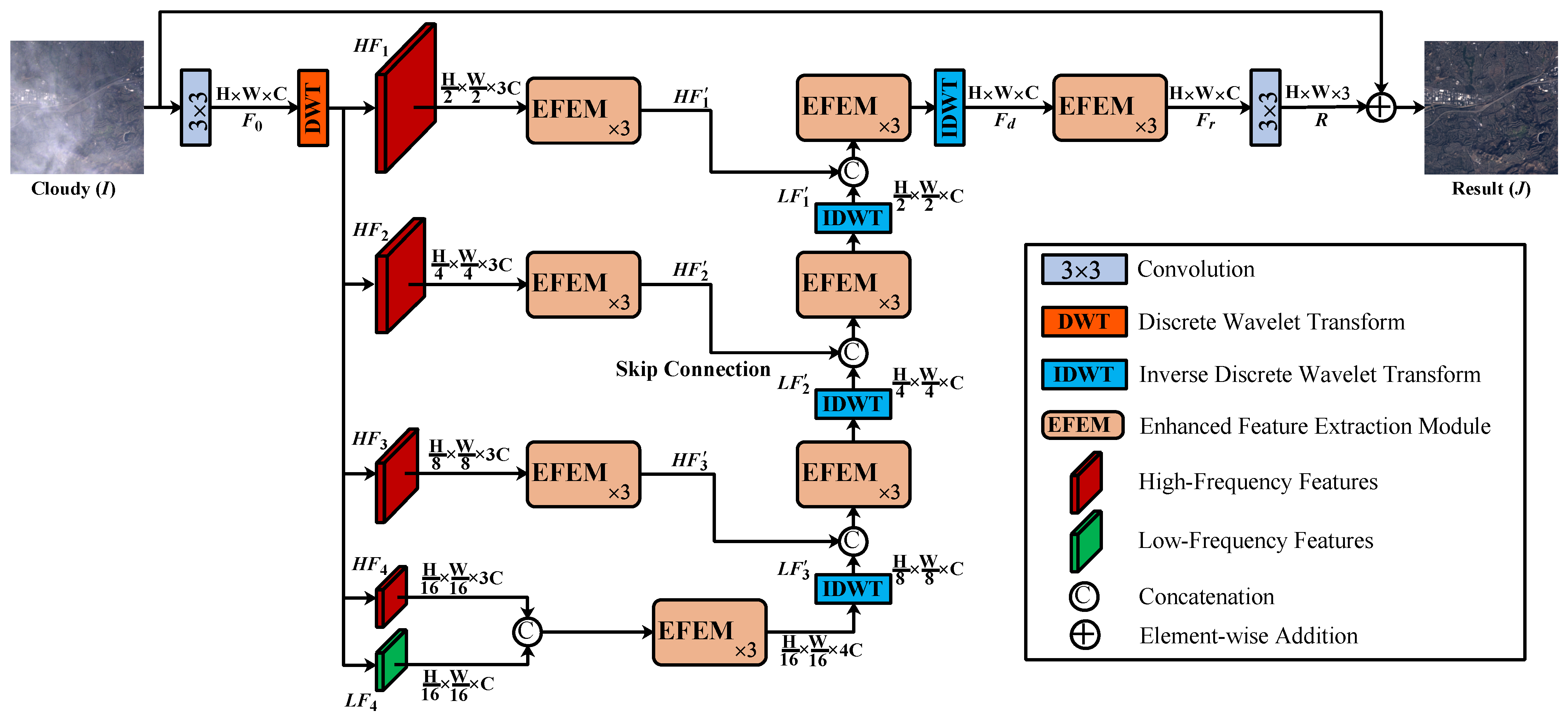
We propose a novel wavelet-integrated CNN for thin cloud removal in RS images, which we call WaveCNN-CR. WaveCNN-CR can obtain multi-scale and multi-frequency features as well as larger receptive fields without any information loss. In addition, it can generate cloud-free results with more accurate details by directly processing the high-frequency features.

2.

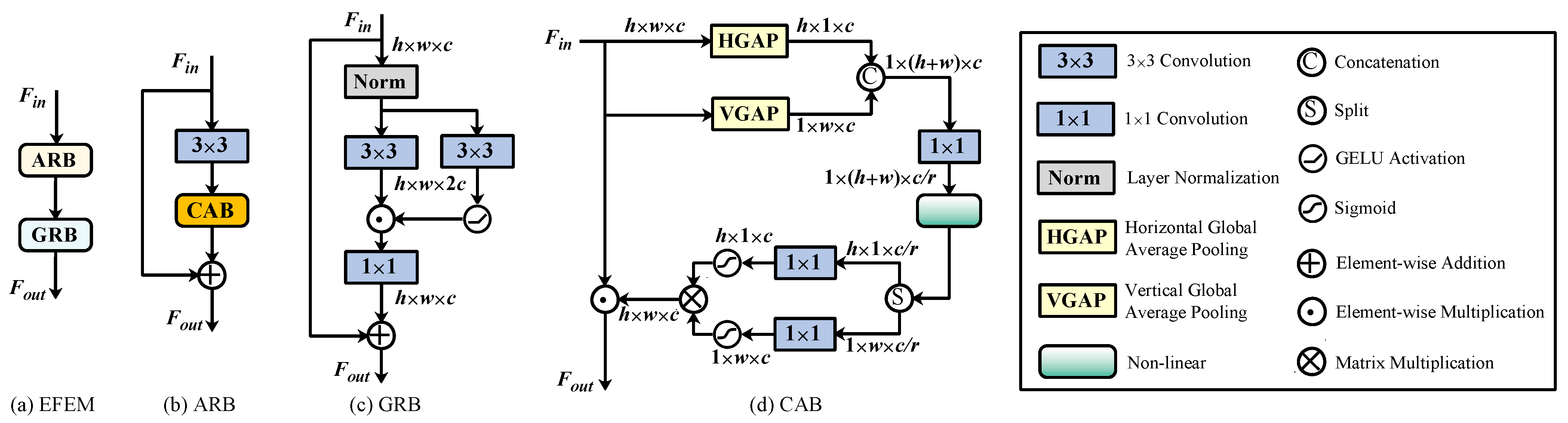
We design a novel EFEM consisting of an attentive residual block (ARB) and gated residual block (GRB) in WaveCNN-CR, enabling stronger feature representation ability. ARB enhances features by capturing long-range interactive global information based on an attention mechanism, while GRB enhances features by exploiting local information based on a gating mechanism.

3.

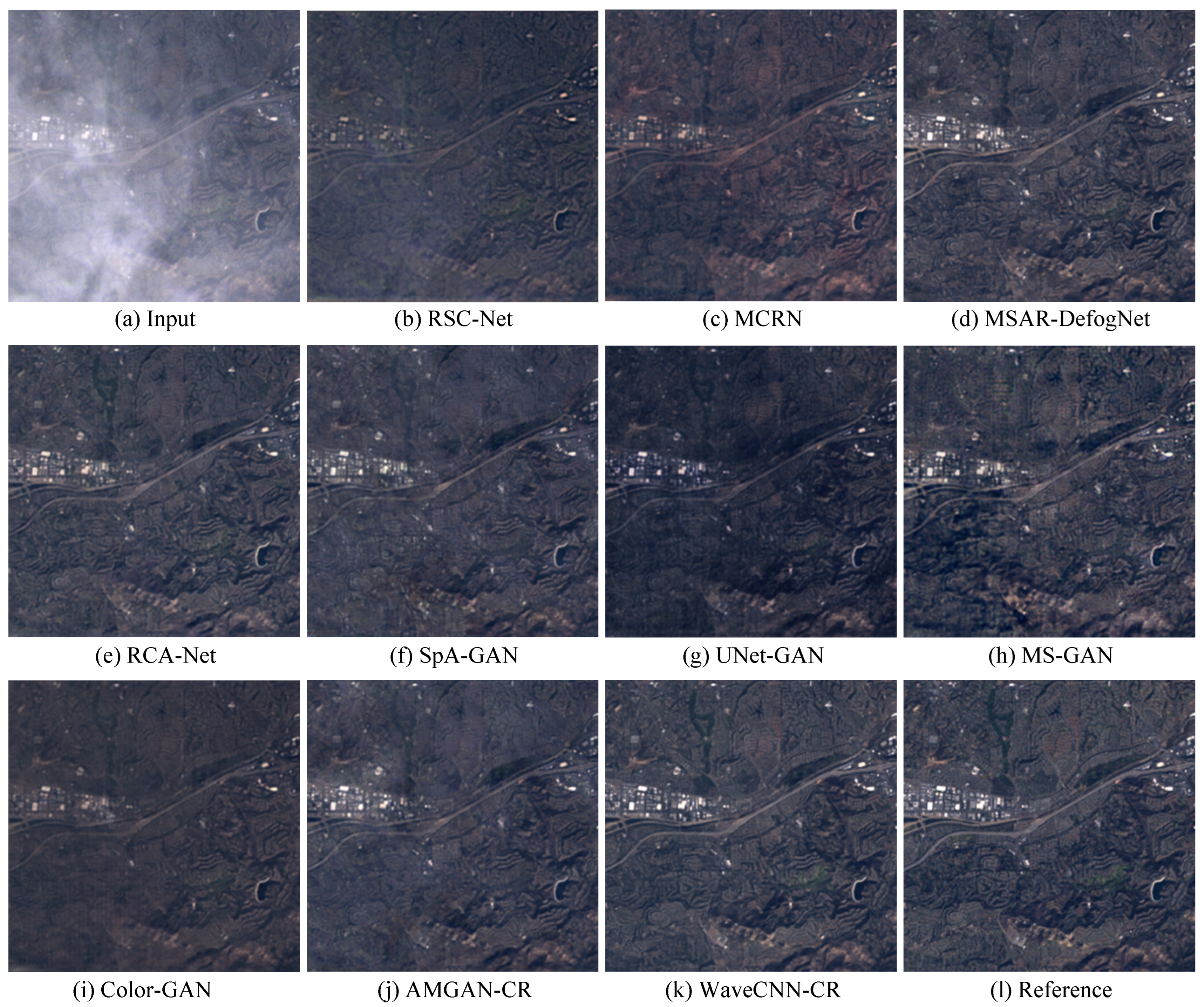
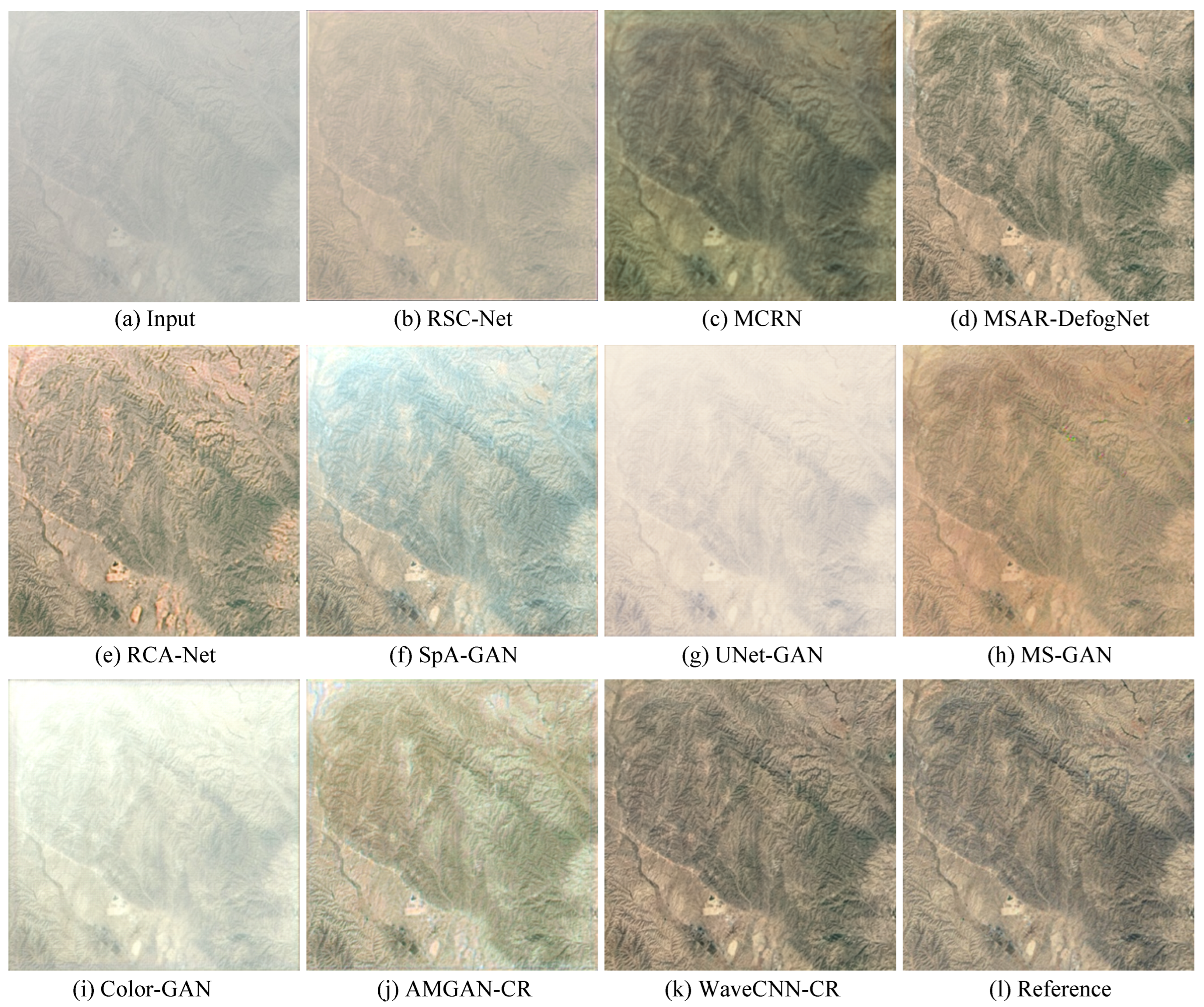
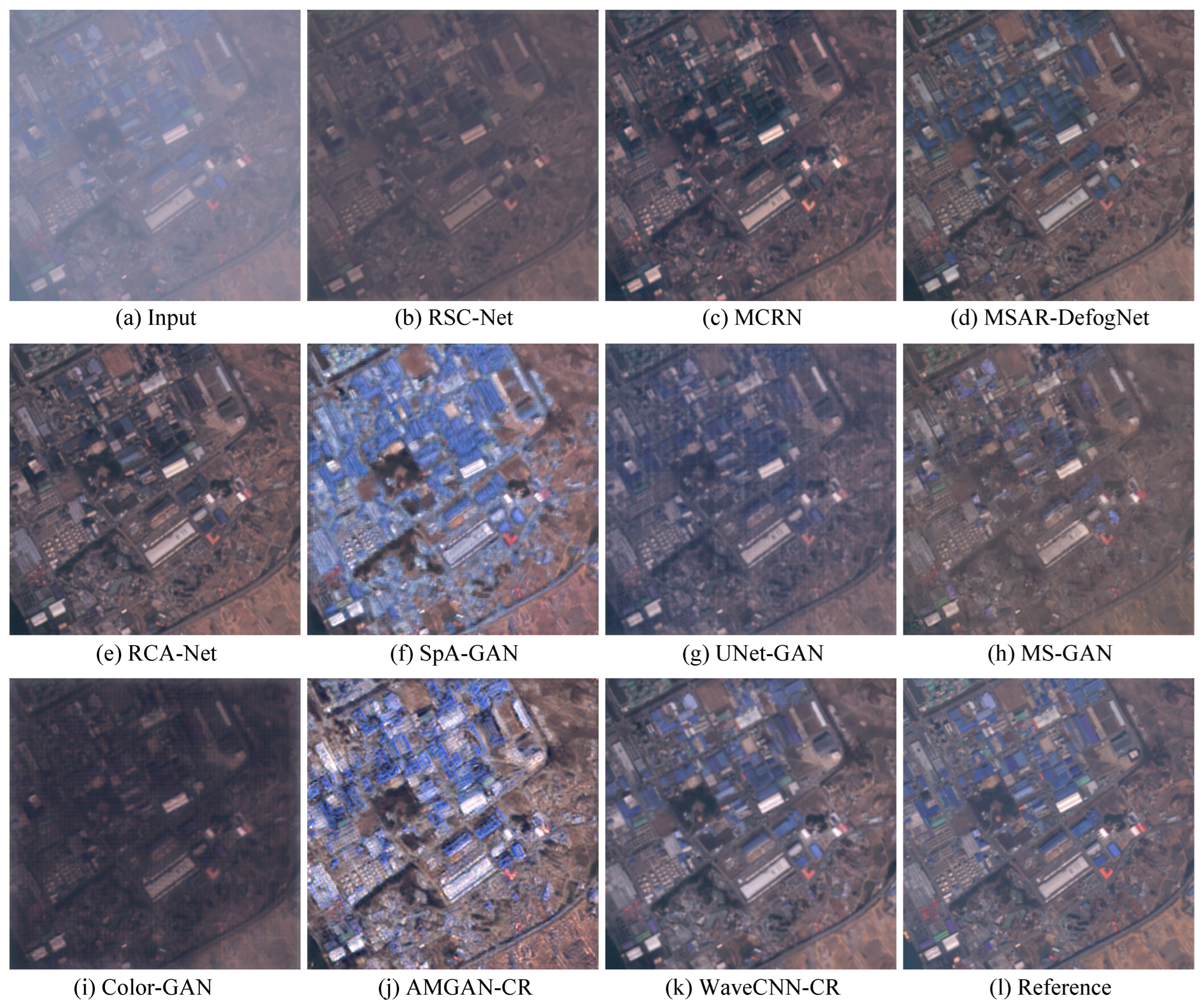
We conduct extensive experiments on three public datasets, T-CLOUD, RICE1, and WHUS2-CR, which respectively include Landsat 8, Google Earth, and Sentinel-2A images. Compared with existing thin cloud removal methods, WaveCNN-CR achieves state-of-the-art (SOTA) results both qualitatively and quantitatively.

The remainder of this paper is organized as follows. Section 2 briefly introduces related works. Section 3 presents details of the proposed thin cloud removal method. Our experimental results and analysis are described and discussed in Section 4. Finally, our conclusions are provided in Section 5.

2. Related Works

Below, we provide a brief analysis of the network architecture of existing DL-based thin cloud removal methods in Section 2.1. In addition, we introduce the application of wavelets to DL-based computer visual tasks in Section 2.2.

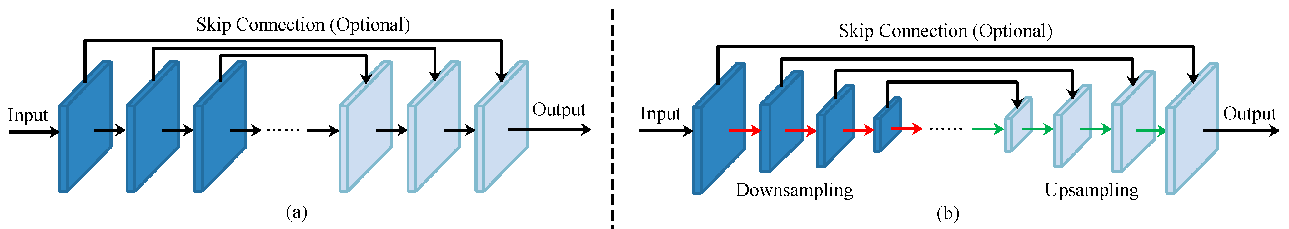
2.1. Network Architecture of Existing DL-Based Methods

Recently, DL-based thin cloud removal methods have achieved amazing results [34,36,47,50]. The major difference between these end-to-end methods lies in their network architectures. There are generally two different main structures: plane encoder–decoder structures [33,34,36,43,45,47] and hourglass-shaped encoder–decoder structures [35,38,39,40,41,44,48,50,51]. The former retains feature maps with the same spatial dimensions as the input image in both the encoder and decoder without any downsampling or upsampling operations (see Figure 1a), which can preserve image details without information loss. However, it has limited receptive fields and lacks the long-range dependencies of image and context, which is not conducive to the removal of nonuniform thin clouds [55]. The latter structure gradually reduces the size of the feature maps via downsampling operations in the encoder, then increases the size of the feature maps via upsampling operations in the decoder (see Figure 1b), which can obtain larger receptive fields and multi-scale features. Nevertheless, the downsampling operation (strided-convolution/pooling) damages image details and causes loss of detail information; furthermore, existing upsampling operations (deconvolution/interpolation) cannot accurately recover the original data, which is not conducive to the restoration of image detail [56].

A predominant thin cloud removal method needs to effectively remove thin clouds from the whole image while avoiding corruption of image details. This requires a thin cloud removal model with both large receptive fields and no loss of detail information. Existing methods fail to balance the tradeoff between large receptive fields and preservation of image detail. To address this problem, in this paper our proposed WaveCNN-CR employs wavelet transform instead of conventional downsampling operations to enlarge the receptive field without any information loss, then inverse wavelet transform is used to reconstruct the high-resolution feature maps. In addition, direct processing of the high-frequency features obtained by the wavelet transform facilitates the recovery of image detail.

2.2. Wavelet Transform in DL-Based Computer Vision

Wavelet transform [54] decomposes a signal into different frequency components, which is invertible and information-lossless. Researchers have integrated wavelet transform into CNNs to enhance performance in various computer vision tasks. For example, Huang et al. [57] proposed a wavelet-based CNN to recover the missing details in the wavelet domain for multi-scale face super-resolution. Liu et al. [58] utilized multi-level wavelet transform to enlarge the receptive field without information loss for image restoration. Li et al. [56] designed WaveCNets by replacing conventional downsampling operations with discrete wavelet transform (DWT) to improve the classification accuracy and noise-robustness of CNNs for image classification. For the stripe noise removal task, TSWEU [59] utilized wavelet transform to extract the intrinsically directional feature in the stripe and multi-scale image features; SNRWDNN [60] used quarter-sized wavelet sub-bands as inputs to simultaneously improve the computational efficiency and destriping performance. Chen et al. [61] embedded the dual-tree complex wavelet transform into a CNN for better retrieval of snow information in the single image desnowing task. WaveGAN [62] incorporated wavelet transform and GAN to ameliorate synthesis quality from the frequency domain perspective for few-shot image generation.

Unlike most of these approaches, which generally replace downsampling operations with wavelet transforms, then directly concatenate the low-frequency and high-frequency components and feed them into the convolution layer for feature extraction, our proposed WaveCNN-CR adopts multi-level wavelet transform to decompose the input features into multi-scale frequency components and perform feature extraction for each frequency component separately in the encoding stage. Then, the processed low-frequency and high-frequency components are combined and gradually restored to their original resolution by inverse DWT (IDWT) in the decoding stage.

3. Method

In this paper, we propose a thin cloud removal method for RS images using a wavelet-integrated CNN, WaveCNN-CR. First, we present the overall framework of WaveCNN-CR in Section 3.1. Then, in Section 3.2 we describe the hierarchical wavelet transform in WaveCNN-CR. Moreover, we elaborate the architecture of ARB and GRB in detail in Section 3.3 and Section 3.4, respectively. Finally, we introduce the loss function of WaveCNN-CR in Section 3.5.

3.1. Overall Framework

The framework of the proposed WaveCNN-CR is shown in Figure 2. Considering a cloudy RGB image $I\in {\mathbb{R}}^{H\times W\times 3}$ with spatial dimensions $H\times W$, WaveCNN-CR first employs a $3\times 3$ convolution operation to obtain low-level features $F_0\in {\mathbb{R}}^{H\times W\times C}$, where C is the number of channels. Then, the hierarchical wavelet transform is applied to decompose the shallow features $F_0$ into four levels of high-frequency components, i.e., ${HF}_1\in {\mathbb{R}}^{\frac{H}{2}\times \frac{W}{2}\times 3C}$, ${HF}_2\in {\mathbb{R}}^{\frac{H}{4}\times \frac{W}{4}\times 3C}$, ${HF}_3\in {\mathbb{R}}^{\frac{H}{8}\times \frac{W}{8}\times 3C}$, and ${HF}_4\in {\mathbb{R}}^{\frac{H}{16}\times \frac{W}{16}\times 3C}$, along with a low-frequency component ${LF}_4\in {\mathbb{R}}^{\frac{H}{16}\times \frac{W}{16}\times C}$. Next, ${HF}_1$, ${HF}_2$, and ${HF}_3$ pass directly through three consecutive EFEMs to obtain deep features. The proposed EFEM consists of an ARB and a GRB (see Figure 3a). At each level in the decoding stage, the low-frequency features are first concatenated with high-frequency features and then passed through three EFEMs, before finally being converted into the low-frequency features of the upper level by IDWT. Therefore, the low-resolution image features are gradually recovered as high-resolution features. After four IDWT operations, WaveCNN-CR obtains enriched deep features $F_d\in {\mathbb{R}}^{H\times W\times C}$ with the same spatial dimensions as the input image, and $F_d$ are further refined using three EFEMs at high spatial resolution. Finally, WaveCNN-CR utilizes a $3\times 3$ convolution to transform the refined feature $F_r$ into a residual image $R\in {\mathbb{R}}^{H\times W\times 3}$ and generates a clear image $J=I+R$ by global residual learning.

3.2. Hierarchical Wavelet Transform

Wavelet transform provides information on both frequency and spatiality without any information loss, which is crucial for accurate thin cloud removal and image detail preservation. WaveCNN-CR adopts a simple yet effective wavelet transform, namely, Haar wavelet [63]. Haar wavelet contains two operations (i.e., DWT and IDWT) and four wavelet filters, i.e., a low-pass filter $f_{LL}$ and high-pass filters $f_{LH}$, $f_{HL}$, and $f_{HH}$.

$$f_{LL}=\frac{1}{2}\left[\begin{array}{cc}1& 1\\ 1& 1\end{array}\right],f_{LH}=\frac{1}{2}\left[\begin{array}{cc}-1& -1\\ 1& 1\end{array}\right],f_{HL}=\frac{1}{2}\left[\begin{array}{cc}-1& 1\\ -1& 1\end{array}\right],f_{HH}=\frac{1}{2}\left[\begin{array}{cc}1& -1\\ -1& 1\end{array}\right]$$

(1)

The low-pass filter focuses on low-frequency image structure information. In contrast, the high-pass filters capture high-frequency image detail and texture information.

First, we extract multi-scale and multi-frequency wavelet features by four-level DWT and recursively invert the processed multi-scale features to reconstruct an initial resolution output by IDWT, as shown in Figure 2. Specifically, the shallow features $F_0$ are decomposed into a quarter-sized low-frequency component $L{L}_1$ and high-frequency components ${LH}_1$, ${HL}_1$, and ${HH}_1$ via DWT in the first level, which can be formulated as

$${LL}_1=F_0⊛f_{LL},{LH}_1=F_0⊛f_{LH},{HL}_1=F_0⊛f_{HL},{HH}_1=F_0⊛f_{HH}$$

(2)

where ⊛ represents the convolution operation. Then, the decomposition continues iteratively on ${LL}_{i-1}$ to produce ${LL}_i$, ${LH}_i$, ${HL}_i$, and ${HH}_i(i=2,3,4)$. Hence, we obtain a total of one low-frequency component and twelve multi-scale high-frequency components. We take ${LL}_4$ as the low-frequency features ${LF}_4$ and concatenate ${LH}_i$, ${HL}_i$, and ${HH}_i$ in the channel dimension as the ith level high-frequency features ${HF}_i$. In the decoding stage, we iteratively concatenate $L{F}_i$ and $H{F}_i$, feed them into the EFEM for feature extraction, then apply IDWT to reconstruct $L{F}_{i-1}(i=4,3,2,1)$.

3.3. Attentive Residual Block

Attention mechanisms are widely used in various computer vision tasks, such as image classification, object detection, image denoising, and thin cloud removal, and can effectively improve the learning ability of CNNs. Attention enhances feature representation by recalibrating the feature maps to emphasize useful features and suppress useless features. In addition, RL can directly transfer features from shallow layers to deeper layers through skip connection. In particular, for the thin cloud removal task RL can avoid corruption of clear ground information. Meanwhile, RL allows CNNs with greater depth to be trained more easily. Inspired by this, we combined an attention mechanism with RL in our proposed attentive residual block for enhanced feature extraction.

The architecture of our proposed ARB is shown in Figure 3b, and its mathematical formula can be expressed as

$$F_{out}=Att\left(W^{3\times 3}\left(F_{in}\right)\right)+F_{in}$$

(3)

$$W^{3\times 3}\left(F_{in}\right)=F_{in}⊛\omega$$

(4)

where $F_{in}$ and $F_{out}$ are the input and output feature maps of ARB, respectively, $Att(·)$ represents the attention block, $W^{3\times 3}$ denotes the $3\times 3$ convolution, and the convolution kernel $\omega$ is the parameter of the network. First, $\omega$ is assigned initial values by random initialization and then gradually optimized by backpropagation according to the loss function in the training stage. ARB first employs a convolutional layer for feature extraction, then aggregates global contextual information for feature enhancement through the attention block. In this paper, we utilize the coordinate attention block (CAB) [64], which can obtain channel attention and global spatial attention simultaneously by integrating the horizontal attention and vertical attention. CAB performs better than the classical SE channel attention block [65] and CBAM [66] because SE contains only channel attention, while CBAM calculates channel attention and local spatial attention separately.

Figure 3d presents the architecture of CAB. With an input tensor $F_{in}\in {\mathbb{R}}^{h\times w\times c}$, two one-dimensional global average pooling operations are first used to aggregate the input features along the horizontal and vertical directions, respectively. The resulting two direction-aware feature maps $F_h\in {\mathbb{R}}^{h\times 1\times c}$ and $F_w\in {\mathbb{R}}^{1\times w\times c}$ can then be formulated as

$$F_h=HGAP\left(F_{in}\right)$$

(5)

$$F_w=VGAP\left(F_{in}\right)$$

(6)

where $HGAP$ and $VGAP$ refer to horizontal global average pooling and vertical global average pooling, respectively. Then, $F_h$ and $F_w$ are concatenated and encoded by a $1\times 1$ convolutional layer and a nonlinear activation layer, which can be written as

$$F_{enc}=\delta \left(W^{1\times 1}\left([F_h,F_w]\right)\right)$$

(7)

$$\delta \left(X\right)=X·\phi (X+3)/6$$

(8)

where $[·,·]$ represents the concatenation along the spatial dimension, $W^{1\times 1}$ denotes the $1\times 1$ convolution, $\phi$ is the non-linear activation function ReLU6 [67], and $F_{enc}\in {\mathbb{R}}^{1\times (h+w)\times c/r}$ are the output encoded feature maps. Here, r is the channel reduction ratio. Then, $F_{enc}$ are split along the spatial dimension into two separate feature maps, $F_{enc}^h\in {\mathbb{R}}^{h\times 1\times c/r}$ and $F_{enc}^w\in {\mathbb{R}}^{1\times w\times c/r}$. An additional two $1\times 1$ convolution operations are used to convert $F_{enc}^h$ and $F_{enc}^w$ into tensors with the same number of channels as $F_{in}$, respectively, and the following sigmoid function is used for normalization, obtaining

$$g_h=\sigma \left(W_h^{1\times 1}\left(F_{enc}^h\right)\right)$$

(9)

$$g_w=\sigma \left(W_w^{1\times 1}\left(F_{enc}^w\right)\right)$$

(10)

where $\sigma$ is the sigmoid function and $g_h$ and $g_w$ are the horizontal and vertical attention weights, respectively. Finally, $g_h$ and $g_w$ are combined to rescale the input features $F_{in}$, and the output of CAB can be written as

$$F_{out}=F_{in}\odot (g_h\otimes g_w)$$

(11)

where ⊙ and ⊗ denote elementwise multiplication and matrix multiplication, respectively.

3.4. Gated Residual Block

After ARB obtains the enhanced features using the global context information, we further apply the gating mechanism to control the flow of features based on the local context information. The gating mechanism can be modeled as the element-wise multiplication of two parallel paths of $3\times 3$ convolutional layers, one of which is followed by a nonlinear activation layer. The architecture of our proposed GRB is illustrated in Figure 3c. With an input tensor $F_{in}\in {\mathbb{R}}^{h\times w\times c}$, GRB can be formulated as

$$F_{out}=W^{1\times 1}\left(Gating\left(F_{in}\right)\right)+F_{in}$$

(12)

$$Gating\left(F_{in}\right)=W_1^{3\times 3}\left(\psi \left(F_{in}\right)\right)\odot \varphi \left(W_2^{3\times 3}\left(\psi \left(F_{in}\right)\right)\right)$$

(13)

$$\psi \left(F_{in}^l\right)=\frac{F_{in}^l-{\mu }^l}{\sqrt{{\left({\sigma }^l\right)}^2+ϵ}}·g^l+b^l(l=1,2,...,c)$$

(14)

where $\psi$ and $\varphi$ are the layer normalization [68] and GELU nonlinearity [69], respectively, $F_{in}^l$ denotes the l-th channel of the input tensor, ${\mu }^l$ and ${\left({\sigma }^l\right)}^2$ are the mean and variance of $F_{in}^l$, respectively, $ϵ$ is a small constant that prevent the denominator from being zero, and $g^l$ and $b^l$ are two learnable parameters. Here, it is worth noting that we first use two $3\times 3$ convolutions to expand the channels of the layer normalized features by a factor of two in order to exploit richer local features, then finally reduce the channels back to the original input dimension by a $1\times 1$ convolution. Overall, GRB allows us to choose which part of the features should be propagated to the next layer of the network. Specific to the thin cloud removal task, thanks to global residual learning this means allowing information relating to clouds to pass forward while blocking information on cloud-free regions, resulting in better thin cloud removal performance and better fidelity in cloud-free regions.

3.5. Loss Function

The $L_1$ norm and mean squared error (MSE) are the most commonly used loss functions in supervised image-to-image translation tasks. However, the minimization of MSE suppresses high-frequency detail information, causing the phenomenon of regression to the mean and resulting in blurred and oversmoothed results [70,71]. Therefore, in this paper we employ $L_1$ loss to optimize WaveCNN-CR. The loss function can be expressed as

$$L\left(\omega \right)=\frac{1}{N}\sum _{i=1}^N{∥f_{\omega }\left(I_i\right)-G{T}_i∥}_1$$

(15)

where $I_i$ and ${GT}_i$ are the ith thin cloud image and corresponding ground truth (cloud-free reference image) in the training set, respectively, N is the number of training samples, $\left|\right|•|{|}_1$ represents the $L_1$ norm, $f_{\omega }$ denotes our WaveCNN-CR, and $\omega$ represents the parameters of WaveCNN-CR. Here, we aim to minimize $L\left(\omega \right)$ in order to obtain the optimal parameters ${\omega }^{*}$.

$${\omega }^{*}=arg\underset{\omega }{min}L\left(\omega \right)$$

(16)

4. Results and Discussion

In this part, we first describe the experimental settings, including the datasets, evaluation metrics, and implementation details, in Section 4.1. Next, the ablution study on the T-CLOUD dataset is presented and discussed in Section 4.2. Finally, we conduct comparative experiments with other SOTA methods in Section 4.3.

4.1. Experimental Setting

4.1.1. Datasets

In our experiments, we evaluated our method on three public datasets: T-CLOUD [37], RICE [72], and WHUS2-CR [35].

Table 1. Properties of the T-CLOUD, RICE1, and WHUS2-CR datasets used in the experiments.

Dataset	Source	Size	Training	Test	Type
T-CLOUD	Landsat 8	$256\times 256$	2351	588	Nonuniform
RICE1	Google Earth	$512\times 512$	400	100	Uniform
WHUS2-CR	Sentinel-2A	$256\times 256$	4000	1000	Nonuniform

summarizes the similarities and differences of these three datasets.

(1) T-CLOUD dataset: The data in T-CLOUD are from Landsat 8 RGB images. The dataset contains 2939 doublets of cloudy images and their clear counterparts separated by one satellite re-entry period (16 days). At first, the original optical RS image pairs are captured by the same satellite sensor at different times. Then, the image sub-regions which have similar lighting conditions on the corresponding cloudy and cloud-free images are selected to form the training and testing data. Finally, the paired cloudy and cloud-free images can be obtained by cropping at the corresponding position. All images are cropped to a size of $256\times 256$ pixels. The data are split with a ratio of 8:2, with 2351 images in the training set and 588 images in the test set.

(2) RICE dataset: RICE contains two subsets: thin cloud-contaminated RICE1 and thick cloud-contaminated RICE2. The former consists of 500 pairs of cloudy images and their cloud-free counterparts, all with a size of $512\times 512$, while the latter has 450 triplets of images, each triplet containing a reference image without clouds, a thick cloud-covered image, and the mask of the clouds. We chose RICE1 for our thin cloud removal experiments. In RICE1, all images are collected from Google Earth by setting whether or not to exhibit the cloud layer. We randomly selected 400 pairs for training and the remaining 100 pairs for testing.

(3) WHUS2-CR dataset: In the WHUS2-CR dataset, cloudy and corresponding cloud-free images are captured by the Sentinel-2A satellite, which has a multispectral imager for ground exploration. To reduce the difference between cloudy and cloud-free images as much as possible, the time lag of the acquisition dates of cloudy and corresponding cloud-free images is set to ten days, which is the revisitation time of the Sentinel-2A satellite. In WHUS2-CR, we randomly cropped 5000 image patches with a size of $256\times 256$ pixels from the original high-resolution image pairs. In our experiments, 4000 pairs were used for training and 1000 pairs for testing.

4.1.2. Evaluation Metrics

To quantitatively evaluate the performance of thin cloud removal methods, we adopted the widely used peak signal-to-noise ratio (PSNR) [73], structural similarity (SSIM) [74], and CIEDE2000 [75] as full-reference metrics.

Specifically, PSNR calculates the ratio of the maximum pixel value against the pixel-wise evaluation error, which can be formulated as

$$\mathrm{PSNR}(X,Y)=10·{log}_{10}\frac{{(2^B-1)}^2}{\mathrm{MSE}(X,Y)}$$

(17)

$$\mathrm{MSE}(X,Y)=\frac{1}{N}\left|\right|X-{Y\left|\right|}^2$$

(18)

where MSE is the mean squared error between the thin cloud removal result X and the ground-truth image Y, N is the number of pixels in the image, and B denotes the bit depth of the image, which is generally takes a a value of 8, that is, $2^B-1=255$. A larger PSNR indicates a better thin cloud removal result.

SSIM evaluates the similarity between two images in terms of luminance, contrast, and structure:

$$\mathrm{SSIM}(X,Y)=l(X,Y)·c(X,Y)·s(X,Y)$$

(19)

$$l(X,Y)=\frac{2{\mu }_X{\mu }_Y+c_1}{{\mu }_X^2+{\mu }_Y^2+c_1}$$

(20)

$$c(X,Y)=\frac{2{\sigma }_X{\sigma }_Y+c_2}{{\sigma }_X^2+{\sigma }_Y^2+c_2}$$

(21)

$$s(X,Y)=\frac{{\sigma }_{XY}+c_3}{{\sigma }_X{\sigma }_Y+c_3}$$

(22)

where ${\mu }_X$ and ${\mu }_Y$ are the mean values of X and Y, respectively, ${\sigma }_X^2$ and ${\sigma }_Y^2$ are the variances of X and Y, respectively, ${\sigma }_{XY}$ is the covariance of X and Y, and $c_1$, $c_2$, and $c_3$ are small constants that prevent the denominator term from being zero. The value of SSIM ranges from 0 to 1, with larger values indicating a better thin cloud removal effect.

CIEDE2000 measures the color difference between two images, which is consistent with subjective human visual perception. CIEDE2000 can be defined as

$$\mathrm{CIEDE}2000(X,Y)=\sqrt{{\left(\frac{\Delta L^{{}^{\prime }}}{k_L{S}_L}\right)}^2+{\left(\frac{\Delta C^{{}^{\prime }}}{k_C{S}_C}\right)}^2+{\left(\frac{\Delta H^{{}^{\prime }}}{k_H{S}_H}\right)}^2+R_T\left(\frac{\Delta C^{{}^{\prime }}}{k_C{S}_C}\right)\left(\frac{\Delta H^{{}^{\prime }}}{k_H{S}_H}\right)}$$

(23)

where $\Delta L^{{}^{\prime }}$, $\Delta C^{{}^{\prime }}$, and $\Delta H^{{}^{\prime }}$ are the CIELAB metrics lightness, chroma, and hue differences between X and Y, respectively; $k_L$, $k_C$, and $k_H$ are the parametric factors; and the weighting factors $S_L$, $S_C$, and $S_H$ and interactive term $R_T$ are calculated from $\Delta L^{{}^{\prime }}$, $\Delta C^{{}^{\prime }}$, and $\Delta H^{{}^{\prime }}$, respectively. For detailed calculations, refer to [76]. A smaller value of CIEDE2000 indicates better color preservation.

4.1.3. Implementation Details

The proposed WaveCNN-CR was implemented in PyTorch and trained on an Intel Gold 6252 CPU and an NVIDIA A100 GPU. The number of channels in the first convolution layer was set to $C=48$, and the channel reduction ratio in CAB was set to $r=4$. We trained WaveCNN-CR with the Adam [77] optimizer (${\beta }_1=0.9$, ${\beta }_2=0.999$). The batch size and training epochs were set to 1 and 300, respectively. The initial learning rate was set to 0.0003 for the first 100 epochs, then gradually reduced to 0 over the next 200 epochs using the cosine annealing strategy [78]. In addition, we used horizontal and vertical flipping for data augmentation.

4.2. Ablation Study

To verify the effectiveness of the proposed WaveCNN-CR, we conducted extensive ablation experiments to analyze the overall architecture of WaveCNN-CR and the structure of EFEM, ARB, and GRB. The T-CLOUD dataset was employed for training and testing. For fast comparisons, the training epochs in all ablation experiments were set to 150.

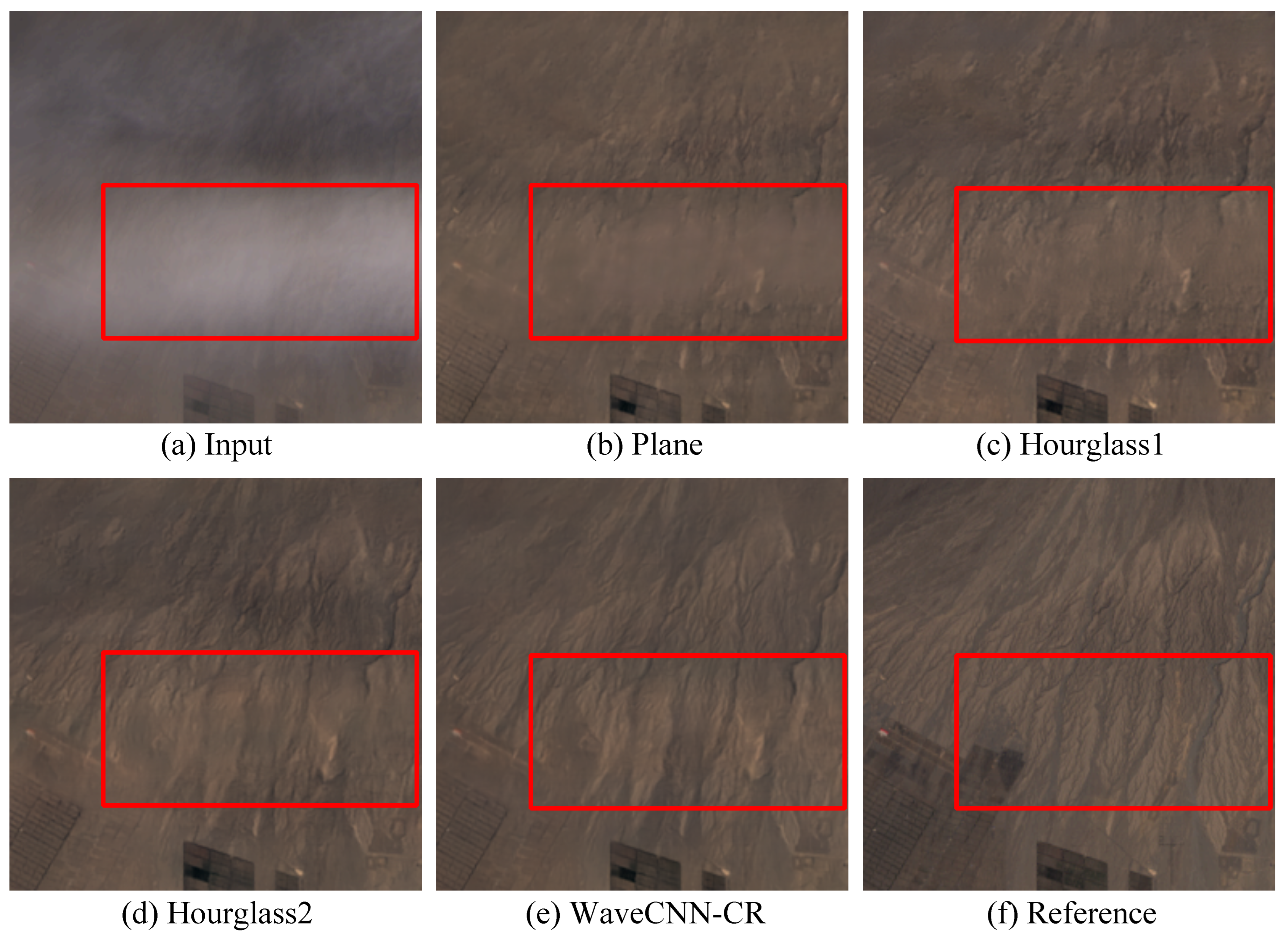
4.2.1. Analysis of Overall Architecture

To demonstrate the effectiveness of wavelet transform in WaveCNN-CR, we compared it with three variant models without wavelet transform. One of the variants was designed with the plane structure (denoted as Plane) and the other two variants adopted the hourglass-shaped structure, one utilizing convolution and deconvolution with stride 2 as the respective downsampling and upsampling operations (denoted as Hourglass1) and the other using average pooling as the downsampling operation and bilinear interpolation as the upsampling operation (denoted as Hourglass2). In Hourglass2, we employed 1 × 1 convolution before downsampling and upsampling to ensure that the number of channels in its feature map was consistent with that in WaveCNN-CR. The qualitative comparison results are shown in Figure 4. Plane was limited by the small receptive fields, resulting in unsatisfactory result on nonuniform thin clouds (see the red box area). Hourglass2 performed better than Hourglass1, effectively removing the nonuniform thin clouds, though there were blurry detail textures in its results. In contrast, our proposed WaveCNN-CR benefited from the wavelet transform without information loss, effectively removing the nonuniform thin clouds while accurately recovering the detailed texture of the image.

Table 2. Ablution analysis of the overall architecture of WaveCNN-CR. The bold and underlined text indicates the best and second-best performance, respectively. The ↑ symbol indicates that larger values are better, while ↓ indicates that smaller values are better.

Architecture	PSNR↑	SSIM↑	CIEDE2000↓
Plane	30.15	0.8681	3.7293
Hourglass1	29.45	0.8492	4.1804
Hourglass2	30.43	0.8676	3.6911
WaveCNN-CR	31.01	0.8813	3.4262

presents the quantitative results. It can be seen that compared with Hourglass2, Plane performed poorly in terms of PSNR and CIEDE2000, while performing better on the SSIM metric. This is because there were no downsampling/upsampling operations in Plane, thereby protecting the detailed texture of the image. Our proposed WaveCNN-CR is able to integrated wavelet transform into CNN, achieving the best results on all three evaluation metrics.

4.2.2. Effectiveness of EFEM

In the proposed WaveCNN-CR, EFEM consists of an ARB followed by a GRB. To verify the effectiveness of EFEM, we compared it with three variants: (1) two ARBs (denoted ARB_ARB), (2) two GRBs (denoted GRB_GRB), and (3) one GRB followed by one ARB (denoted GRB_ARB). As shown in

Table 3. Ablution analysis of the structure of EFEM. The bold and underlined text indicates the best and second-best performance, respectively. The ↑ symbol indicates that larger values are better, while ↓ indicates that smaller values are better.

EFEM	PSNR↑	SSIM↑	CIEDE2000↓
ARB_ARB	28.41	0.8440	4.3556
GRB_GRB	30.58	0.8783	3.5269
GRB_ARB	30.85	0.8792	3.4644
Ours(ARB_GRB)	31.01	0.8813	3.4262

, the results of the combination of ARB and GRB were better than those of two ARBs or GRBs alone, indicating that global ARB and local GRB are complementary. The proposed EFEM composed of ARB and GRB in sequence, achieved the best results, which also proves that this global–local enhancement strategy can obtain higher performance gains.

4.2.3. Analysis of ARB

To verify the effectiveness of the ARB, we compared it with variant modules with different structures. In

Table 4. Ablution analysis of the structure of ARB. The bold and underlined text indicates the best and second-best performance, respectively. The ↑ symbol indicates that larger values are better, while ↓ indicates that smaller values are better.

Block	PSNR↑	SSIM↑	CIEDE2000↓
CB	28.65	0.8547	4.2068
AB	29.14	0.8359	4.3878
RB	28.84	0.8600	4.1158
ARB_SE	30.64	0.8777	3.5421
ARB_CBAM	30.27	0.8742	3.6667
Ours(ARB_CAB)	31.01	0.8813	3.4262

, CB denotes a regular convolutional block without an attention mechanism or residual connection, while AB and RB represent an attentive block with attention mechanism and residual block with residual connection, respectively. In addition, ARB_SE and ARB_CBAM represent ARBs with SE and CBAM attention modules, respectively. From the quantitative comparison results, it can be seen that, as compared with CB, RB obtained better results, while AB achieved higher PSNR gains while showing poor performance in terms of SSIM and CIEDE2000. The later three ARBs with different attention mechanisms were significantly better than the first three, illustrating the effectiveness of combining the attention mechanism and RL. Our ARB using CAB achieved the best results, with 31.01 dB in PSNR, 0.8813 in SSIM, and 3.4262 in CIEDE2000.

4.2.4. Analysis of GRB

We conducted experiments to verify the effectiveness of GRB. As shown in

Table 5. Ablution analysis of the structure of GRB. The bold and underlined text indicates the best and second-best performance, respectively. The ↑ symbol indicates that larger values are better, while ↓ indicates that smaller values are better.

Block	PSNR↑	SSIM↑	CIEDE2000↓
CB	26.80	0.8134	5.2177
GB	25.50	0.7727	5.9063
RB	29.68	0.8626	3.9105
Ours(GRB)	31.01	0.8813	3.4262

, CB represents the convolutional block without a gating mechanism or residual connection, while GB and RB denote the gated block with gating mechanism and residual block with residual connection, respectively. GB performed the worst, indicating that the gating mechanism plays a negative role when there is no residual connection. Based on RB, our GRB with gating mechanism showed improved performance of 1.33 dB PSNR, 0.0187 SSIM, and 0.4843 CIEDE2000.

4.3. Comparisons with SOTA Methods

In this section, we present the experimental results on the T-CLOUD, RICE1, and WHUS2-CR datasets used to evaluate our proposed WaveCNN-CR. Quantitative and qualitative comparisons were conducted against several SOTA methods, including four CNN-based methods (RSC-Net [33], MCRN [50], MSAR-DefogNet [36], and RCA-Net [34]) and five GAN-based methods (SpA-GAN [45], UNet-GAN [38], MS-GAN [39], Color-GAN [44], and AMGAN-CR [47]).

The quantitative results are presented in

Table 6. Quantitative evaluations on the T-CLOUD dataset. The bold and underlined text indicates the best and second-best performance, respectively. The ↑ symbol indicates that larger values are better, while ↓ indicates that smaller values are better.

Method	PSNR↑	SSIM↑	CIEDE2000↓
RSC-Net [33]	23.98	0.7596	7.0502
MCRN [50]	26.60	0.8091	5.5816
MSAR-DefogNet [36]	28.84	0.8432	4.1862
RCA-Net [34]	28.69	0.8443	4.3708
SpA-GAN [45]	27.15	0.8145	4.9107
UNet-GAN [38]	23.71	0.7630	7.6156
MS-GAN [39]	24.04	0.7228	7.8543
Color-GAN [44]	24.01	0.7490	6.9769
AMGAN-CR [47]	27.85	0.8317	4.5691
WaveCNN-CR	31.21	0.8838	3.3479

,

Table 7. Quantitative evaluations on the RICE1 dataset. The bold and underlined text indicates the best and second-best performance, respectively. The ↑ symbol indicates that larger values are better, while ↓ indicates that smaller values are better.

Method	PSNR↑	SSIM↑	CIEDE2000↓
RSC-Net [33]	21.34	0.8150	8.3078
MCRN [50]	31.09	0.9465	3.3767
MSAR-DefogNet [36]	33.58	0.9534	2.7066
RCA-Net [34]	32.49	0.9537	2.2334
SpA-GAN [45]	29.62	0.8844	4.3374
UNet-GAN [38]	23.92	0.8085	7.6766
MS-GAN [39]	27.74	0.8796	5.6267
Color-GAN [44]	21.57	0.8065	8.5284
AMGAN-CR [47]	29.05	0.8965	4.4694
WaveCNN-CR	35.74	0.9650	1.7922

and

Table 8. Quantitative evaluations on the WHUS2-CR dataset. The bold and underlined text indicates the best and second-best performance, respectively. The ↑ symbol indicates that larger values are better, while ↓ indicates that smaller values are better.

Method	PSNR↑	SSIM↑	CIEDE2000↓
RSC-Net [33]	29.03	0.9056	4.6571
MCRN [50]	28.81	0.9163	4.7939
MSAR-DefogNet [36]	29.89	0.9168	5.2028
RCA-Net [34]	29.57	0.9128	4.4211
SpA-GAN [45]	28.78	0.8887	4.7904
UNet-GAN [38]	29.58	0.9008	5.1388
MS-GAN [39]	27.59	0.8560	6.2101
Color-GAN [44]	29.24	0.9020	4.7212
AMGAN-CR [47]	28.82	0.8672	4.9061
WaveCNN-CR	30.29	0.9318	4.1469

. It can be seen that the five attention-based methods, including MSAR-DefogNet, RCA-Net, SpA-GAN, AMGAN-CR, and WaveCNN-CR, significantly outperformed the remaining five methods without an attention mechanism, proving the effectiveness of the attention mechanism. Our proposed WaveCNN-CR achieved remarkable performance gains over existing methods on all three datasets. Compared to the most recent best method, MSAR-DefogNet, WaveCNN-CR achieved improvements of 2.37 dB, 2.16 dB, and 0.40 dB PSNR and 0.0406, 0.0116, and 0.0150 SSIM on the T-CLOUD, RICE1, and WHUS2-CR datasets, respectively. For the color difference indicator, CIEDE2000, the quantitative results consistently showed that WaveCNN-CR achieveds the best performance, demonstrating that WaveCNN-CR has great potential to improve thin cloud removal performance.

In addition, we calculated the average pixel values of the input cloudy images, reference images, and results of different methods on the three test datasets, as shown in

Table 9. Statistical results of the average pixel values of the input cloudy images, reference images, and results of different methods on the three test datasets.

Method	T-CLOUD			RICE1			WHUS2-CR
	Red	Green	Blue	Red	Green	Blue	Red	Green	Blue
Input	101.31	96.71	106.93	131.09	130.98	127.39	80.89	87.73	98.41
RSC-Net [33]	67.12	62.52	69.52	128.08	124.34	114.84	64.54	68.89	75.71
MCRN [50]	70.55	63.31	69.93	118.80	118.29	105.75	66.20	69.84	75.30
MSAR-DefogNet [36]	71.77	65.64	71.95	122.96	120.69	110.56	66.18	70.49	76.18
RCA-Net [34]	69.64	64.42	70.24	121.06	119.94	108.56	66.64	71.25	76.99
SpA-GAN [45]	69.96	64.27	70.78	121.56	121.36	110.28	66.52	72.74	78.78
UNet-GAN [38]	67.24	62.31	72.29	125.87	123.24	117.82	64.08	69.22	75.87
MS-GAN [39]	66.92	62.19	69.60	118.87	116.90	107.60	62.92	67.85	73.04
Color-GAN [44]	69.94	63.96	71.16	119.16	123.26	108.43	64.18	68.28	75.67
AMGAN-CR [47]	70.14	64.48	70.93	122.04	120.38	109.37	66.01	69.75	74.57
WaveCNN-CR	70.78	64.88	71.13	122.34	120.43	109.70	65.05	69.79	75.00
Reference	71.09	65.14	71.35	122.48	120.68	109.85	64.59	70.03	76.45

. It can be observed that all the thin cloud removal results were darker than the input cloudy image. The results of WaveCNN-CR had the closest average pixel values to the reference images, indicating that our WaveCNN-CR achieved the best thin cloud removal results.

Qualitative comparisons of each method are shown in Figure 5, Figure 6 and Figure 7. In Figure 5, we compared the cloud removal capabilities of various methods on the nonuniform T-CLOUD dataset. The visual results show that RSC-Net suffered from cloud residue, MCRN had noticeable color distortion, and grid-like artifacts were observed in UNet-GAN. While the thin cloud removal results from GAN-based methods had few residual clouds, the difference from the reference image was relatively large, such as with Color-GAN, which may be due to the instability of GANs during training. On the other hand, MSAR-DefogNet, RCA-Net, and WaveCNN-CR all generated satisfactory cloud-free results, with our WaveCNN-CR having more accurate details and more consistent colors when compared to the reference image. Overall, WaveCNN-CR achieved the best results in terms of thin cloud removal, image detail recovery, and color fidelity.

Figure 6 shows the visual results of a heavily thin cloud-contaminated image in the uniform RICE1 dataset. The results indicate that RSC-Net, SpA-GAN, UNet-GAN, and Color-GAN suffered from many remaining clouds. The remaining five methods, MCRN, MSAR-DefogNet, RCA-Net, MS-GAN, and AMGAN-CR, all obtained cloud-free results, although with varying degrees of color deviation compared to the reference image. The restored image obtained with the proposed WaveCNN-CR had more similar patterns to the reference image, with no color distortion, which is consistent with the quantitative results. Furthermore, a thin cloud removal instance of a moderately thin cloud-contaminated image in the WHUS2-CR dataset is shown in Figure 7. It can be observed that while all comparison methods suffered from varying degrees of color distortion, the visual quality of the restoration results demonstrates the superiority of WaveCNN-CR.

Furthermore, we compared the parameters, computational cost, and test time of different methods on the T-CLOUD dataset, with the results shown in

Table 10. Parameters, computational cost, and test time of different methods on the T-CLOUD dataset.

Image	Parameters (M)	FLOPs (G)	Test Time (ms)
RSC-Net [33]	0.11	14.84	8.06
MCRN [50]	1.41	94.90	44.68
MSAR-DefogNet [36]	0.80	104.90	6.11
RCA-Net [34]	2.27	401.79	21.33
SpA-GAN [45]	0.21	33.97	19.03
UNet-GAN [38]	3.31	11.83	4.89
MS-GAN [39]	8.08	44.27	10.83
Color-GAN [44]	0.51	9.95	5.58
AMGAN-CR [47]	0.29	96.96	16.05
WaveCNN-CR	30.38	395.09	40.23

. It can be seen that RSC-Net, UNet-GAN, MS-GAN, and Color-GAN had relatively lower computational costs and time consumption, however, their thin cloud removal performance was relatively poor. While MCRN, RCA-Net, SpA-GAN, and AMGAN-CR had higher computational and time costs, and their thin cloud removal results were better than those of the previous four methods. MSAR-DefogNet achieved a good balance between parameters, computations, time cost, and the effectiveness of cloud removal. Overall, our WaveCNN-CR had the highest number of parameters and the second-highest cost in terms of computation and time. Compared with MSAR-DefogNet, our WaveCNN-CR made sacrifices in terms of memory usage and time consumption, but showed greatly improved effectiveness in thin cloud removal.

5. Conclusions

In this paper, we proposed a novel thin cloud removal method for RS images, called WaveCNN-CR, that integrates wavelet transform into CNN. Benefiting from the lossless decomposition of wavelet transform, WaveCNN-CR is able to obtain large receptive fields and simultaneously preserve image details, which is an advantage over existing thin cloud removal methods. Specifically, WaveCNN-CR adopts hierarchical DWT to decompose the input features into multi-scale and multi-frequency components, then performs feature extraction for each high-frequency component at different scales using multiple EFEMs in the encoding stage. Then, the processed low-frequency and high-frequency components are recursively combined to reconstruct the high-resolution output in the decoding stage via IDWT. Furthermore, we designed a novel EFEM to integrate global and local information to improve the feature representation ability of WaveCNN-CR. This EFEM is composed of both ARB and GRB; ARB enhances features through the global contextual information captured by attention mechanism, while GRB enhances features through the local contextual information exploited by the gating mechanism. We conducted comparative experiments on three publicly available datasets, T-CLOUD, RICE1, and WHUS2-CR, that include Landsat 8, Google Earth, and Sentinel-2A images, respectively. Both the qualitative and quantitative results demonstrated that WaveCNN-CR significantly outperforms other SOTA methods in terms of thin cloud removal and image detail restoration.

In future work, we intend to apply WaveCNN-CR to multispectral and multitemporal RS images, making full use of spatial, spectral, and temporal information to remove clouds. Additionally, WaveCNN-CR could be applied to other image restoration tasks such as denoising, deblurring, and deraining. Considering that the collection of large datasets with paired images is time-consuming, WaveCNN-CR could be combined with transfer learning on a small dataset or combined with GANs in a weakly supervised way to remove thin clouds from RS images.

References

1. Pan, B.; Shi, Z.; Xu, X.; Shi, T.; Zhang, N.; Zhu, X. CoinNet: Copy initialization network for multispectral imagery semantic segmentation. IEEE Geosci. Remote Sens. Lett. 2018, 16, 816–820. [Google Scholar] [CrossRef]
2. Shi, L.; Wang, Z.; Pan, B.; Shi, Z. An end-to-end network for remote sensing imagery semantic segmentation via joint pixel-and representation-level domain adaptation. IEEE Geosci. Remote Sens. Lett. 2020, 18, 1896–1900. [Google Scholar] [CrossRef]
3. Chen, J.; Xie, F.; Lu, Y.; Jiang, Z. Finding arbitrary-oriented ships from remote sensing images using corner detection. IEEE Geosci. Remote Sens. Lett. 2019, 17, 1712–1716. [Google Scholar] [CrossRef]
4. Liu, E.; Zheng, Y.; Pan, B.; Xu, X.; Shi, Z. DCL-Net: Augmenting the capability of classification and localization for remote sensing object detection. IEEE Trans. Geosci. Remote Sens. 2021, 59, 7933–7944. [Google Scholar] [CrossRef]
5. Zhu, Z.; Woodcock, C.E. Continuous change detection and classification of land cover using all available Landsat data. Remote Sens. Environ. 2014, 144, 152–171. [Google Scholar] [CrossRef] [Green Version]
6. Chen, H.; Shi, Z. A spatial-temporal attention-based method and a new dataset for remote sensing image change detection. Remote Sens. 2020, 12, 1662. [Google Scholar] [CrossRef]
7. Benz, U.C.; Hofmann, P.; Willhauck, G.; Lingenfelder, I.; Heynen, M. Multi-resolution, object-oriented fuzzy analysis of remote sensing data for GIS-ready information. ISPRS J. Photogramm. Remote Sens. 2004, 58, 239–258. [Google Scholar] [CrossRef]
8. Zhang, Y.; Rossow, W.B.; Lacis, A.A.; Oinas, V.; Mishchenko, M.I. Calculation of radiative fluxes from the surface to top of atmosphere based on ISCCP and other global data sets: Refinements of the radiative transfer model and the input data. J. Geophys. Res. Atmos. 2004, 109. [Google Scholar] [CrossRef] [Green Version]
9. King, M.D.; Platnick, S.; Menzel, W.P.; Ackerman, S.A.; Hubanks, P.A. Spatial and temporal distribution of clouds observed by MODIS onboard the Terra and Aqua satellites. IEEE Trans. Geosci. Remote Sens. 2013, 51, 3826–3852. [Google Scholar] [CrossRef]
10. Shen, H.; Li, H.; Qian, Y.; Zhang, L.; Yuan, Q. An effective thin cloud removal procedure for visible remote sensing images. ISPRS J. Photogramm. Remote Sens. 2014, 96, 224–235. [Google Scholar] [CrossRef]
11. Pan, X.; Xie, F.; Jiang, Z.; Yin, J. Haze removal for a single remote sensing image based on deformed haze imaging model. IEEE Signal Process. Lett. 2015, 22, 1806–1810. [Google Scholar] [CrossRef]
12. Li, J.; Hu, Q.; Ai, M. Haze and thin cloud removal via sphere model improved dark channel prior. IEEE Geosci. Remote Sens. Lett. 2018, 16, 472–476. [Google Scholar] [CrossRef]
13. Makarau, A.; Richter, R.; Muller, R.; Reinartz, P. Haze detection and removal in remotely sensed multispectral imagery. IEEE Trans. Geosci. Remote Sens. 2014, 52, 5895–5905. [Google Scholar] [CrossRef] [Green Version]
14. Makarau, A.; Richter, R.; Schlapfer, D.; Reinartz, P. Combined haze and cirrus removal for multispectral imagery. IEEE Geosci. Remote Sens. Lett. 2016, 13, 379–383. [Google Scholar] [CrossRef]
15. He, M.; Wang, B.; Sheng, W.; Yang, K.; Hong, L. Thin cloud removal method in color remote sensing image. Opt. Tech. 2017, 43, 503–508. [Google Scholar]
16. Hu, G.; Li, X.; Liang, D. Thin cloud removal from remote sensing images using multidirectional dual tree complex wavelet transform and transfer least square support vector regression. J. Appl. Remote Sens. 2015, 9, 095053. [Google Scholar] [CrossRef]
17. Shen, Y.; Wang, Y.; Lv, H.; Qian, J. Removal of thin clouds in Landsat-8 OLI data with independent component analysis. Remote Sens. 2015, 7, 11481–11500. [Google Scholar] [CrossRef] [Green Version]
18. Lv, H.; Wang, Y.; Gao, Y. Using independent component analysis and estimated thin-cloud reflectance to remove cloud effect on Landsat-8 oli band data. In Proceedings of the 2018 IEEE International Geoscience and Remote Sensing Symposium (IGARSS), Valencia, Spain, 22–27 July 2018; pp. 915–918. [Google Scholar] [CrossRef]
19. Xu, M.; Jia, X.; Pickering, M.; Jia, S. Thin cloud removal from optical remote sensing images using the noise-adjusted principal components transform. ISPRS J. Photogramm. Remote Sens. 2019, 149, 215–225. [Google Scholar] [CrossRef]
20. Hong, G.; Zhang, Y. Haze removal for new generation optical sensors. Int. J. Remote Sens. 2018, 39, 1491–1509. [Google Scholar] [CrossRef]
21. Lv, H.; Wang, Y.; Shen, Y. An empirical and radiative transfer model based algorithm to remove thin clouds in visible bands. Remote Sens. Environ. 2016, 179, 183–195. [Google Scholar] [CrossRef]
22. Lv, H.; Wang, Y.; Yang, Y. Modeling of thin-cloud TOA reflectance using empirical relationships and two Landsat-8 visible band data. IEEE Trans. Geosci. Remote Sens. 2018, 57, 839–850. [Google Scholar] [CrossRef]
23. Xu, M.; Jia, X.; Pickering, M. Automatic cloud removal for Landsat 8 OLI images using cirrus band. In Proceedings of the 2014 IEEE Geoscience and Remote Sensing Symposium (IGARSS), Quebec City, QC, Canada, 13–18 July 2014; pp. 2511–2514. [Google Scholar] [CrossRef]
24. Zhou, B.; Wang, Y. A thin-cloud removal approach combining the cirrus band and RTM-based algorithm for Landsat-8 OLI data. In Proceedings of the 2019 IEEE Geoscience and Remote Sensing Symposium (IGARSS), Yokohama, Japan, 28 July–2 August 2019; pp. 1434–1437. [Google Scholar] [CrossRef]
25. He, K.; Zhang, X.; Ren, S.; Sun, J. Deep residual learning for image recognition. In Proceedings of the 2016 IEEE Conference on Computer Vision and Pattern Recognition (CVPR), Las Vegas, NV, USA, 27–30 June 2016; pp. 770–778. [Google Scholar] [CrossRef] [Green Version]
26. Que, Y.; Dai, Y.; Jia, X.; Leung, A.K.; Chen, Z.; Tang, Y.; Jiang, Z. Automatic classification of asphalt pavement cracks using a novel integrated generative adversarial networks and improved VGG model. Eng. Struct. 2023, 277, 115406. [Google Scholar] [CrossRef]
27. Redmon, J.; Divvala, S.; Girshick, R.; Farhadi, A. You only look once: Unified, real-time object detection. In Proceedings of the 2016 IEEE Conference on Computer Vision and Pattern Recognition (CVPR), Las Vegas, NV, USA, 27–30 June 2016; pp. 779–788. [Google Scholar] [CrossRef] [Green Version]
28. Wu, F.; Duan, J.; Ai, P.; Chen, Z.; Yang, Z.; Zou, X. Rachis detection and three-dimensional localization of cut off point for vision-based banana robot. Comput. Electron. Agric. 2022, 198, 107079. [Google Scholar] [CrossRef]
29. Long, J.; Shelhamer, E.; Darrell, T. Fully convolutional networks for semantic segmentation. In Proceedings of the 2015 IEEE Conference on Computer Vision and Pattern Recognition (CVPR), Boston, MA, USA, 7–12 June 2015; pp. 3431–3440. [Google Scholar] [CrossRef] [Green Version]
30. Zhao, H.; Shi, J.; Qi, X.; Wang, X.; Jia, J. Pyramid scene parsing network. In Proceedings of the 2017 IEEE Conference on Computer Vision and Pattern Recognition (CVPR), Honolulu, HI, USA, 21–26 July 2017; pp. 2881–2890. [Google Scholar] [CrossRef] [Green Version]
31. Isola, P.; Zhu, J.Y.; Zhou, T.; Efros, A.A. Image-to-image translation with conditional adversarial networks. In Proceedings of the 2017 IEEE Conference on Computer Vision and Pattern Recognition (CVPR), Honolulu, HI, USA, 21–26 July 2017; pp. 1125–1134. [Google Scholar] [CrossRef]
32. Zhu, J.Y.; Park, T.; Isola, P.; Efros, A.A. Unpaired image-to-image translation using cycle-consistent adversarial networks. In Proceedings of the 2017 IEEE International Conference on Computer Vision (ICCV), Venice, Italy, 22–29 October 2017; pp. 2223–2232. [Google Scholar] [CrossRef] [Green Version]
33. Li, W.; Li, Y.; Chen, D.; Chan, J.C.W. Thin cloud removal with residual symmetrical concatenation network. ISPRS J. Photogramm. Remote Sens. 2019, 153, 137–150. [Google Scholar] [CrossRef]
34. Wen, X.; Pan, Z.; Hu, Y.; Liu, J. An effective network integrating residual learning and channel attention mechanism for thin cloud removal. IEEE Geosci. Remote Sens. Lett. 2022, 19, 6507605. [Google Scholar] [CrossRef]
35. Li, J.; Wu, Z.; Hu, Z.; Li, Z.; Wang, Y.; Molinier, M. Deep learning based thin cloud removal fusing vegetation red edge and short wave infrared spectral information for Sentinel-2A imagery. Remote Sens. 2021, 13, 157. [Google Scholar] [CrossRef]
36. Zhou, Y.; Jing, W.; Wang, J.; Chen, G.; Scherer, R.; Damaševičius, R. MSAR-DefogNet: Lightweight cloud removal network for high resolution remote sensing images based on multi scale convolution. IET Image Process. 2022, 16, 659–668. [Google Scholar] [CrossRef]
37. Ding, H.; Zi, Y.; Xie, F. Uncertainty-based thin cloud removal network via conditional variational autoencoders. In Proceedings of the 2022 Asian Conference on Computer Vision (ACCV), Macau SAR, China, 4–8 December 2022; pp. 469–485. [Google Scholar]
38. Zheng, J.; Liu, X.Y.; Wang, X. Single image cloud removal using U-Net and generative adversarial networks. IEEE Trans. Geosci. Remote Sens. 2020, 59, 6371–6385. [Google Scholar] [CrossRef]
39. Xu, Z.; Wu, K.; Huang, L.; Wang, Q.; Ren, P. Cloudy image arithmetic: A cloudy scene synthesis paradigm with an application to deep-learning-based thin cloud removal. IEEE Trans. Geosci. Remote Sens. 2022, 60, 1–16. [Google Scholar] [CrossRef]
40. Enomoto, K.; Sakurada, K.; Wang, W.; Fukui, H.; Matsuoka, M.; Nakamura, R.; Kawaguchi, N. Filmy cloud removal on satellite imagery with multispectral conditional generative adversarial nets. In Proceedings of the 2017 IEEE Conference on Computer Vision and Pattern Recognition Workshops (CVPRW), Honolulu, HI, USA, 21–26 July 2017; pp. 48–56. [Google Scholar] [CrossRef] [Green Version]
41. Zhang, R.; Xie, F.; Chen, J. Single image thin cloud removal for remote sensing images based on conditional generative adversarial nets. In Proceedings of the Tenth International Conference on Digital Image Processing (ICDIP), Shanghai, China, 11–14 May 2018; Volume 10806, pp. 1400–1407. [Google Scholar] [CrossRef]
42. Mirza, M.; Osindero, S. Conditional generative adversarial nets. arXiv 2014, arXiv:1411.1784. [Google Scholar] [CrossRef]
43. Wen, X.; Pan, Z.; Hu, Y.; Liu, J. Generative adversarial learning in YUV color space for thin cloud removal on satellite imagery. Remote Sens. 2021, 13, 1079. [Google Scholar] [CrossRef]
44. Zhang, C.; Zhang, X.; Yu, Q.; Ma, C. An improved method for removal of thin clouds in remote sensing images by generative adversarial network. In Proceedings of the 2022 IEEE International Geoscience and Remote Sensing Symposium (IGARSS), Kuala Lumpur, Malaysia, 17–22 July 2022; pp. 6706–6709. [Google Scholar] [CrossRef]
45. Pan, H. Cloud removal for remote sensing imagery via spatial attention generative adversarial network. arXiv 2020, arXiv:2009.13015. [Google Scholar] [CrossRef]
46. Chen, H.; Chen, R.; Li, N. Attentive generative adversarial network for removing thin cloud from a single remote sensing image. IET Image Process. 2021, 15, 856–867. [Google Scholar] [CrossRef]
47. Xu, M.; Deng, F.; Jia, S.; Jia, X.; Plaza, A.J. Attention mechanism-based generative adversarial networks for cloud removal in Landsat images. Remote Sens. Environ. 2022, 271, 112902. [Google Scholar] [CrossRef]
48. Xu, Z.; Wu, K.; Ren, P. Recovering thin cloud covered regions in GF satellite images based on cloudy image arithmetic+. In Proceedings of the 2022 IEEE International Geoscience and Remote Sensing Symposium (IGARSS), Kuala Lumpur, Malaysia, 17–22 July 2022; pp. 1800–1803. [Google Scholar] [CrossRef]
49. Zi, Y.; Xie, F.; Zhang, N.; Jiang, Z.; Zhu, W.; Zhang, H. Thin cloud removal for multispectral remote sensing images using convolutional neural networks combined with an imaging model. IEEE J. Sel. Top. Appl. Earth Obs. Remote Sens. 2021, 14, 3811–3823. [Google Scholar] [CrossRef]
50. Yu, W.; Zhang, X.; Pun, M.O.; Liu, M. A hybrid model-based and data-driven approach for cloud removal in satellite imagery using multi-scale distortion-aware networks. In Proceedings of the 2021 IEEE International Geoscience and Remote Sensing Symposium (IGARSS), Brussels, Belgium, 11–16 July 2021; pp. 7160–7163. [Google Scholar] [CrossRef]
51. Yu, W.; Zhang, X.; Pun, M.O. Cloud removal in optical remote sensing imagery using multiscale distortion-aware networks. IEEE Geosci. Remote Sens. Lett. 2022, 19, 5512605. [Google Scholar] [CrossRef]
52. Li, J.; Wu, Z.; Hu, Z.; Zhang, J.; Li, M.; Mo, L.; Molinier, M. Thin cloud removal in optical remote sensing images based on generative adversarial networks and physical model of cloud distortion. ISPRS J. Photogramm. Remote Sens. 2020, 166, 373–389. [Google Scholar] [CrossRef]
53. Zi, Y.; Xie, F.; Song, X.; Jiang, Z.; Zhang, H. Thin cloud removal for remote sensing images using a physical-model-based CycleGAN with unpaired data. IEEE Geosci. Remote Sens. Lett. 2022, 19, 1–5. [Google Scholar] [CrossRef]
54. Mallat, S.G. A theory for multiresolution signal decomposition: The wavelet representation. IEEE Trans. Pattern Anal. Mach. Intell. 1989, 11, 674–693. [Google Scholar] [CrossRef] [Green Version]
55. Yu, H.; Zheng, N.; Zhou, M.; Huang, J.; Xiao, Z.; Zhao, F. Frequency and spatial dual guidance for image dehazing. In Proceedings of the 2022 European Conference on Computer Vision (ECCV), Tel-Aviv, Israel, 23–27 October 2022; pp. 181–198. [Google Scholar] [CrossRef]
56. Li, Q.; Shen, L.; Guo, S.; Lai, Z. Wavelet integrated CNNs for noise-robust image classification. In Proceedings of the 2020 IEEE Conference on Computer Vision and Pattern Recognition (CVPR), Seattle, WA, USA, 13–19 June 2020; pp. 7243–7252. [Google Scholar] [CrossRef]
57. Huang, H.; He, R.; Sun, Z.; Tan, T. Wavelet-SRNet: A wavelet-based CNN for multi-scale face super resolution. In Proceedings of the 2017 IEEE International Conference on Computer Vision (ICCV), Venice, Italy, 22–29 October 2017; pp. 1698–1706. [Google Scholar] [CrossRef]
58. Liu, P.; Zhang, H.; Zhang, K.; Lin, L.; Zuo, W. Multi-level wavelet-CNN for image restoration. In Proceedings of the 2018 IEEE Conference on Computer Vision and Pattern Recognition Workshops (CVPRW), Salt Lake City, UT, USA, 18–22 June 2018; pp. 773–782. [Google Scholar] [CrossRef] [Green Version]
59. Chang, Y.; Chen, M.; Yan, L.; Zhao, X.L.; Li, Y.; Zhong, S. Toward universal stripe removal via wavelet-based deep convolutional neural network. IEEE Trans. Geosci. Remote Sens. 2019, 58, 2880–2897. [Google Scholar] [CrossRef]
60. Guan, J.; Lai, R.; Xiong, A. Wavelet deep neural network for stripe noise removal. IEEE Access 2019, 7, 44544–44554. [Google Scholar] [CrossRef]
61. Chen, W.T.; Fang, H.Y.; Hsieh, C.L.; Tsai, C.C.; Chen, I.H.; Ding, J.J.; Kuo, S.Y. ALL snow removed: Single image desnowing algorithm using hierarchical dual-tree complex wavelet representation and contradict channel loss. In Proceedings of the 2021 IEEE International Conference on Computer Vision (ICCV), Montreal, QC, Canada, 10–17 October 2021; pp. 4176–4185. [Google Scholar] [CrossRef]
62. Yang, M.; Wang, Z.; Chi, Z.; Feng, W. WaveGAN: Frequency-aware GAN for high-fidelity few-shot image generation. In Proceedings of the 2022 European Conference on Computer Vision (ECCV), Tel-Aviv, Israel, 23–27 October 2022; pp. 1–17. [Google Scholar] [CrossRef]
63. Haar, A. Zur theorie der orthogonalen funktionensysteme. Math. Ann. 1911, 71, 38–53. [Google Scholar] [CrossRef]
64. Hou, Q.; Zhou, D.; Feng, J. Coordinate attention for efficient mobile network design. In Proceedings of the 2021 IEEE Conference on Computer Vision and Pattern Recognition (CVPR), Nashville, TN, USA, 20–25 June 2021; pp. 13708–13717. [Google Scholar] [CrossRef]
65. Hu, J.; Shen, L.; Sun, G. Squeeze-and-excitation networks. In Proceedings of the 2018 IEEE Conference on Computer Vision and Pattern Recognition (CVPR), Salt Lake City, UT, USA, 18–22 June 2018; pp. 7132–7141. [Google Scholar] [CrossRef] [Green Version]
66. Woo, S.; Park, J.; Lee, J.Y.; Kweon, I.S. CBAM: Convolutional block attention module. In Proceedings of the 2018 European Conference on Computer Vision (ECCV), Munich, Germany, 8–14 September 2018; pp. 3–19. [Google Scholar] [CrossRef] [Green Version]
67. Howard, A.G.; Zhu, M.; Chen, B.; Kalenichenko, D.; Wang, W.; Weyand, T.; Andreetto, M.; Adam, H. Mobilenets: Efficient convolutional neural networks for mobile vision applications. arXiv 2017, arXiv:1704.04861. [Google Scholar] [CrossRef]
68. Ba, J.L.; Kiros, J.R.; Hinton, G.E. Layer normalization. arXiv 2016, arXiv:1607.06450. [Google Scholar] [CrossRef]
69. Hendrycks, D.; Gimpel, K. Gaussian error linear units (gelus). arXiv 2016, arXiv:1606.08415. [Google Scholar] [CrossRef]
70. Gondal, M.W.; Scholkopf, B.; Hirsch, M. The unreasonable effectiveness of texture transfer for single image super-resolution. In Proceedings of the 2018 European Conference on Computer Vision (ECCV), Munich, Germany, 8–14 September 2018; pp. 80–97. [Google Scholar] [CrossRef] [Green Version]
71. Lim, B.; Son, S.; Kim, H.; Nah, S.; Lee, K.M. Enhanced deep residual networks for single image super-resolution. In Proceedings of the 2017 IEEE Conference on Computer Vision and Pattern Recognition Workshops (CVPRW), Honolulu, HI, USA, 21–26 July 2017; pp. 136–144. [Google Scholar] [CrossRef] [Green Version]
72. Lin, D.; Xu, G.; Wang, X.; Wang, Y.; Sun, X.; Fu, K. A remote sensing image dataset for cloud removal. arXiv 2019, arXiv:1901.00600. [Google Scholar] [CrossRef]
73. Huynh-Thu, Q.; Ghanbari, M. Scope of validity of PSNR in image/video quality assessment. Electron. Lett. 2008, 44, 800–801. [Google Scholar] [CrossRef]
74. Wang, Z.; Bovik, A.C.; Sheikh, H.R.; Simoncelli, E.P. Image quality assessment: From error visibility to structural similarity. IEEE Trans. Image Process. 2004, 13, 600–612. [Google Scholar] [CrossRef] [Green Version]
75. Luo, M.R.; Cui, G.; Rigg, B. The development of the CIE 2000 colour-difference formula: CIEDE2000. Color Res. Appl. 2001, 26, 340–350. [Google Scholar] [CrossRef]
76. Sharma, G.; Wu, W.; Dalal, E.N. The CIEDE2000 color-difference formula: Implementation notes, supplementary test data, and mathematical observations. Color Res. Appl. 2005, 30, 21–30. [Google Scholar] [CrossRef]
77. Kingma, D.P.; Ba, J. Adam: A method for stochastic optimization. arXiv 2014, arXiv:1412.6980. [Google Scholar] [CrossRef]
78. He, T.; Zhang, Z.; Zhang, H.; Zhang, Z.; Xie, J.; Li, M. Bag of tricks for image classification with convolutional neural networks. In Proceedings of the 2019 IEEE Conference on Computer Vision and Pattern Recognition (CVPR), Long Beach, CA, USA, 15–20 June 2019; pp. 558–567. [Google Scholar] [CrossRef]
Figure 1. The two types of network structures used in existing DL-based methods: (a) plane encoder–decoder structure and (b) hourglass-shaped encoder–decoder structure.
Remotesensing 15 00781 g001
Figure 2. The overall framework of the proposed WaveCNN-CR.
Remotesensing 15 00781 g002
Figure 3. Detailed architecture of the modules in WaveCNN-CR: (a) enhanced feature extraction module, (b) attentive residual block, (c) gated residual block, and (d) coordinate attention block.
Remotesensing 15 00781 g003
Figure 4. Visual comparisons of different network architectures: (a) input cloudy image; (be) respective results of Plane, Hourglass1, Hourglass2, and WaveCNN-CR; (f) reference cloud-free image.
Remotesensing 15 00781 g004
Figure 5. Visual comparisons on the T-CLOUD dataset: (a) input cloudy image; (bk) results of RSC-Net [33], MCRN [50], MSAR-DefogNet [36], RCA-Net [34], SpA-GAN [45], UNet-GAN [38], MS-GAN [39], Color-GAN [44], AMGAN-CR [47], and our proposed WaveCNN-CR, respectively; (l) reference cloud-free image.
Remotesensing 15 00781 g005
Figure 6. Visual comparisons on the RICE1 dataset: (a) input cloudy image; (bk) results of RSC-Net [33], MCRN [50], MSAR-DefogNet [36], RCA-Net [34], SpA-GAN [45], UNet-GAN [38], MS-GAN [39], Color-GAN [44], AMGAN-CR [47], and our proposed WaveCNN-CR, respectively; (l) reference cloud-free image.
Remotesensing 15 00781 g006
Figure 7. Visual comparisons on the WHUS2-CR dataset: (a) input cloudy image; (bk) results of RSC-Net [33], MCRN [50], MSAR-DefogNet [36], RCA-Net [34], SpA-GAN [45], UNet-GAN [38], MS-GAN [39], Color-GAN [44], AMGAN-CR [47], and our proposed WaveCNN-CR, respectively; (l) reference cloud-free image.
Remotesensing 15 00781 g007